A novel sandwich algorithm for empirical Bayes analysis of rank data

Abstract

Rank data arises frequently in marketing, finance, organizational behavior, and psychology. Most analysis of rank data reported in the literature assumes the presence of one or more variables (sometimes latent) based on whose values the items are ranked. In this paper we analyze rank data using a purely probabilistic model where the observed ranks are assumed to be perturbed versions of the true rank and each perturbation has a specific probability of occurring. We consider the general case when covariate information is present and has an impact on the rankings. An empirical Bayes approach is taken for estimating the model parameters. The Gibbs sampler is shown to converge very slowly to the target posterior distribution and we show that some of the widely used empirical convergence diagnostic tools may fail to detect this lack of convergence. We propose a novel, fast mixing sandwich algorithm for exploring the posterior distribution. An EM algorithm based on Markov chain Monte Carlo (MCMC) sampling is developed for estimating prior hyperparameters. A real life rank data set is analyzed using the methods developed in the paper. The results obtained indicate the usefulness of these methods in analyzing rank data with covariate information.

Key words and phrases:  Algebraic-Probabilistic model; Convergence; Gibbs sampler; Markov chains; MCMC; Permutation; Rank data; Sandwich algorithm.

1 Introduction

The phenomenon of ranking a given set of items according to some attributes is well known. Students are ranked routinely according to their proficiency in some subject, job applicants are ranked according to their suitability for a particular job, various brands of soap are ranked by consumers according to their intention to purchase them at some later time, various mutual funds are ranked by the investors according to their intention to invest money in them etc. In some cases, like ranking of students for their proficiency in a given subject one may use some objective criterion like the marks scored in an appropriately designed examination for assigning the rank - the student who gets the highest marks gets rank 1, the student who gets the next highest marks gets rank 2 etc. However, in other cases, like the case of evaluating a job applicant, usually more than one attribute is considered. Typically a panel of experts evaluate the items (the candidates) on a variety of relevant dimensions some of which may be objective while others are subjective. Often the individual experts are only able to provide a ranking of the items as perceived by them during the evaluation process. The whole group of experts then considers all the rankings by the individual experts and tries to arrive at a consensus ranking through some subjective decision making process. We call this generally accepted rank the “true rank”. The number of items to be ranked by an expert (a.k.a. subject) is typically small since the “robustness of ranking may well fall if the subject is required to rank a large number of items simultaneously” (Brown, 1974, p.19). Along the same lines Russell and Gray (1994, p. 81), states that forcing subjects to give a different rank to each item may “overtax their true powers of differentiation, with the result that the rank differences they give do not reflect true value differences, but merely add to the noise in the data.” Laha and Dongaonkar (2009) provide a statistical method to derive the “true rank” based on the rankings provided by the individual experts. In this paper we extend this method to the case when the true rank depends on some covariates.

When there are no covariates on the experts, we denote the true rank as $\pi$ and the ranking given by the $i$th expert as $y_{i}$. The ranking $y_{i}$ can be considered as a ‘perturbed’ version of $\pi$ i.e. we assume that $y_{i}=\sigma_{i}\circ\pi$ where $\sigma_{i}\in\mathfrak{S}_{p}$, the set (group) of permutations of the integers $1,2,\dots,p$. The permutations $\sigma_{i}$’s are assumed to be independently distributed $\mathfrak{S}_{p}$ valued random variables following some common law. Laha and Dongaonkar (2009) discuss the estimation of $\pi$ using a Bayesian approach and the Sampling Importance Resampling (SIR) technique.

Suppose now that there are covariates on the experts and the true rank depends on the value of the covariate. Let $X$ be the covariate and suppose it takes the value $x_{i}$ for the $i$th expert. In this case, we have the model $y_{i}=\sigma_{i}\circ\pi(x_{i})$ where as before $\sigma_{i}$’s are i.i.d. $\mathfrak{S}_{p}$ valued random variables. We are interested in estimating $\pi(x)$ where $x\in Range(X)$.

There are several other methods in the literature for analyzing rank data most of which do not incorporate covariates. Models based on order-statistics are discussed in Thurstone (1927), Yellot (1977), Critchlow (1980), Daniels (1950), Mosteller (1951) and Yu (2000). Order-statistics based models consider a latent utility $y_{i}$, of $i$th item, $i=1,\ldots,p$ given by a expert who ranks the items in decreasing order of utility. While some of them assume that for a given expert the variables $y_{i}$’s are independent, Yu (2000) considers a multivariate normal model for the utilities with non-identity covariance matrix. He also considers the case when covariates are associated with items and experts. Models based on distance are first considered in Mallows (1957). These models are further studied in Feigin and Cohen (1978) and Diaconis (1988). Further work in distance based models has been reported in Fligner and Verducci (1986). Mallows model has been generalized by Lebanon and Lafferty (2002). Fligner and Verducci (1988) proposed multistage ranking model where they introduced the concept of central ranking $\pi$ but without any covariates. Recently, mixtures of distance-based models have been considered in Murphy and Martin (2003). An approach based on mixture of experts model to cluster voters in Irish election background has been recently considered in Gormley and Murphy (2008). The mixture of experts model can include covariates (see also Gormley and Murphy, 2010). Also other methods for analyzing rank data without covariates using group representation have been studied in Diaconis (1989). However, our approach of estimating the true rank is not considered elsewhere and is innovative in this regard.

We develop a flexible conjugate prior for Bayesian inference. The use of conjugate prior allows us to construct a Gibbs sampler with standard conditional distributions. Although it is shown that the Gibbs sampler is a uniformly ergodic Markov chain, it converges very slowly to the target posterior distribution because it moves between the modes of the posterior too infrequently (see e.g. Meyn and Tweedie, 1993, for definition of uniformly ergodic Markov chain). On the other hand, this lack of convergence is not detected by a popular Markov chain Monte Carlo (MCMC) empirical convergence diagnostic tool, namely the potential scale reduction factor introduced by Gelman and Rubin (1992). Even though the Gibbs sampler is stuck in a local mode, the autocorrelation (between iterations of the Gibbs chain) is close to zero even before lag three. Only when the Gibbs sampler is run for a very large number (more than five million) of iterations, it visits other modes and the autocorrelations jump to near one showing lack of mixing. This is an alarming issue as in practice, MCMC users employ these empirical convergence diagnostic tools to determine MCMC simulation length and we show that inference drawn from prematurely stopped MCMC simulation may be far from the truth. These observations demonstrate the danger in depending purely on empirical convergence diagnostic tools to verify convergence of MCMC algorithms as these tools may give false indication of convergence.

Every two-variables Gibbs sampler has the same rate of convergence as its two reversible subchains (see e.g. Robert and Casella, 2004; Liu, Wong and Kong, 1994). These subchains can also be viewed as data augmentation (DA) chains (see Hobert and Marchev, 2008). Over the last two decades a lot of effort has gone into modifying DA chains to improve its convergence. These improved algorithms include the parameter expanded DA (PX-DA) algorithm of Liu and Wu (1999), the conditional and marginal augmentation algorithms of Meng and van Dyk (1999), the sandwich algorithm of Hobert and Marchev (2008) and finally the interweaving algorithms of Yu and Meng (2011). Here we consider Hobert and Marchev’s (2008) sandwich techniques to improve the subchains of our Gibbs sampler. In a sandwich algorithm, an extra step is added (sandwiched) to the Gibbs sampler in between the draws from the conditional distributions. We construct a sandwich algorithm and use the Rao-Blackwellization technique to make inference about the true rank, $\pi$. Using results in Hobert, Roy and Robert (2011) we show that all the (ordered) eigenvalues of the Markov operator corresponding to the sandwich chain are less than or equal to the corresponding eigenvalues of the DA Markov operator. We also present an EM algorithm based on MCMC sampling to make inference about the prior hyperparameter.

The structure of the paper is as follows: In Section 2, we introduce the probabilistic rank model with covariates and discuss estimation of the model parameters using a Bayesian approach. In Section 2.1, we build prior distributions on the parameters and provide the joint and marginal posterior distributions (up to normalizing constants). Section 3 contains construction of MCMC algorithms as well as the EM algorithm for estimating the prior hyperparameter. Section 4 demonstrates the convergence issues of the Gibbs sampler through simulation examples. We also describe how our sandwich algorithm results in huge improvement in mixing by adding an extra step to facilitate moves between the modes of the posterior. In Section 5, we discuss analysis of a real life dataset using methods developed earlier in the paper. Some concluding remarks are given in Section 6.

2 An algebraic–probabilistic model

Let us think of a situation in which $p$ items are ranked by a random sample of $n$ experts from a population. In the absence of any covariate information, Laha and Dongaonkar (2009) suppose that there is a “true rank” $\pi$ of the $p$ items and the observed ranks are “perturbed” versions of the true rank $\pi$. The perturbation is the composition of a random permutation from the group of all permutations $\mathfrak{S}_{p}$ with the true rank $\pi.$ When there is one or more categorical variable partitioning the population of the experts into few categories, a natural way to extend the model is to assume that there is a true rank associated with each category of experts and the observed ranks are some random perturbed versions of these true ranks. Thus, if there are $g$ categories of experts and $b_{j}$ denotes the number of experts in the $j$th category and $y_{ij}$’s are the ranks observed from the experts in $j$th category, then we assume that there are true ranks $\pi_{1},\pi_{2},\ldots,\pi_{g}$ such that

$$y_{ij}=\sigma_{ij}\circ\pi_{j},\quad i=1,\ldots,b_{j},$$ (1)

for $j=1,\ldots,g,$ where $\sigma_{ij}$’s are i.i.d random permutations having some distribution and are synonymous to random error perturbations. Notice that because composition is the natural group operation on the group $\mathfrak{S}_{p}$, (1) is the natural ANOVA model on the permutation group.

We use the following notations to denote the $p!$ permutations in $\mathfrak{S}_{p}$. Let $\zeta_{j}=j$th ranking in lexicographic order in $\mathfrak{S}_{p}$. So $\zeta_{1}$ is the identity permutation,

$$\zeta_{2}=\left(\begin{array}[]{ccccc}1&2&\cdots&p-1&p\\ 1&2&\cdots&p&p-1\end{array}\right),$$

$$\zeta_{3}=\left(\begin{array}[]{cccccc}1&2&\cdots&p-2&p-1&p\\ 1&2&\cdots&p-1&p-2&p\end{array}\right)$$

and so on. Finally,

$$\zeta_{p!}=\left(\begin{array}[]{ccccc}1&2&\cdots&p-1&p\\ p&p-1&\cdots&2&1\end{array}\right).$$

Next, in order to construct the distribution of the $\sigma_{ij}$’s, suppose they take the value $\zeta_{k}$ with probability $\theta_{k},$ i.e. $P(\sigma=\zeta_{k})=\theta_{k}.$ It is expected that the experts are sensible so that large random error perturbations are less likely to occur than the smaller ones, where we order the permutations by their distance from the identity permutation. Thus, $\theta_{1}$ should be the highest because it is the probability that the observed rank equals to the true rank for any category. Moreover, whenever $\zeta_{k}$ is farther away from $\zeta_{1}$ than $\zeta_{l},$ it is expected that $\theta_{k}$ would be smaller than $\theta_{l}.$ Based on this assumption, we build our prior distribution on the vector $\boldsymbol{\theta}=(\theta_{1},\ldots,\theta_{p!})$ in the next section.

We break our task into three parts. First we construct prior distributions on the parameters necessary for the Bayesian inference. Next we derive the analytic forms of the marginal posterior distributions of the true ranks $\pi_{1},\ldots,\pi_{g}$ and the vector $\boldsymbol{\theta},$ up to a normalizing constant and demonstrate acute challenges present in computing the normalizing constant. In order to avoid the mammoth computational challenge, we construct a powerful MCMC algorithm that enables us to make fast inference.

2.1 Prior distributions

In order to construct a prior on $\boldsymbol{\theta}$ reflecting our belief that the experts are less likely to make big errors, we begin with fixing the notion of big or small perturbations using the Cayley distance on $\mathfrak{S}_{p}$ (Cayley, 1849). The Cayley distance between two permutations $\tau$ and $\alpha$ is defined as

$$d_{C}(\tau,\alpha)=p-|\tau\circ\alpha^{-1}|$$

where $|\tau\circ\alpha^{-1}|$ is the number of cycles in the unique representation of $\tau\circ\alpha^{-1}$ as a product of disjoint cycles. Based on this distance, we call a perturbation $\tau$ smaller than a perturbation $\alpha,$ if $d_{C}(\tau,\zeta_{1})<d_{C}(\alpha,\zeta_{1}).$ Consequently, we take the prior on $\boldsymbol{\theta}$ as a Dirichlet$(a_{1},\ldots,a_{p!})$ distribution because it is the conjugate prior. We set the hyperparameters of this distribution as

$$a_{k}=\exp(\lambda~{}(p-d_{C}(\zeta_{k},\zeta_{1})))=\exp(\lambda|\zeta_{k}|),$$ (2)

where $\lambda>0$ is a parameter that reflects the overall precision in ranking the items. If $\lambda$ is large then the distribution of the error $\sigma$ is concentrated on the set of permutations having many cycles and thus at most a few items are mis-ranked by the experts. In contrast, when the value of $\lambda$ is small, the experts end up mis-ranking a large number of items. This prior distribution on the $\boldsymbol{\theta}$ stems from the natural exponential family on the permutation group McCullagh (2011) which puts a mass proportional to $\exp(\lambda|\zeta_{k}|)$ on the permutation $\zeta_{k}.$ However, had we deterministically set $\theta_{k}\varpropto\exp(\lambda|\zeta_{k}|)$, computations would have been very difficult because the nice conjugacy structure enjoyed by our model would be broken.

In this article, we follow an empirical Bayesian route and estimate the hyperparameter $\lambda$ by maximizing the marginal likelihood $p(\textbf{y}|\lambda),$ the details of which are given in Section 3.4. Estimating $\lambda$ by maximizing the marginal likelihood ensures that the inference remains invariant to multiplying the $a_{k}$’s in (2) by any arbitrary constant.

As far as the prior on the true ranks are concerned, we could incorporate any available knowledge while constructing the prior distribution. For example, if an item is known to be favorite we can construct a prior under which that particular item is more likely to be a top choice. If there is any reason to believe spatial correlation among the true ranks, e.g. for voting data, we can incorporate this information in the prior. For simplicity and ease of computation, however, we would like to assume that the $\pi_{j}$’s are apriori independently distributed and if there is no obvious reason as to why one or more items should be given preference to others, we can keep uniform priors (on $\mathfrak{S}_{p}$). In general, we denote the prior on $\boldsymbol{\pi}\equiv(\pi_{1},\pi_{2},\ldots,\pi_{g})$ by $p(\boldsymbol{\pi})=p_{1}(\pi_{1})p_{2}(\pi_{2})\cdots p_{g}(\pi_{g}).$

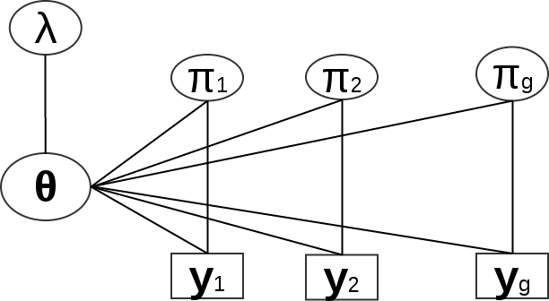
Figure 1: Graphical representation of the algebraic–probabilistic model proposed in this paper. Here $\mathbf{y}_{j}=\{y_{ij},i=1,\ldots,b_{j}\},$ is the collection of all ranks given by experts in the $j$th category; $j=1\ldots,g.$

2.2 Exact posterior and its limitations

It is quite useful to visualize the conditional dependence structure among the variables. This is displayed in Figure 1. Two features are noticeable from the graph. Firstly, $\pi_{j}$’s are conditionally independent among themselves given $\boldsymbol{\theta}$ and the data $\textbf{y}.$ Secondly, the likelihood of $\lambda$ given all other variables depends only on $\boldsymbol{\theta}.$ These two observations will be key ingredients in our computational methods later in the article. To this end, notice that the likelihood of the data is given by

$$p(\textbf{y}|~{}\boldsymbol{\theta},\pi_{1},\ldots,\pi_{g})=\prod_{j=1}^{g}\prod_{i=1}^{p!}\theta_{\zeta_{i}\circ\pi_{j}^{-1}}^{n_{ij}}$$ (3)

where $n_{ij}$ is the number of times the ranking $\zeta_{i}$ is observed in the $j$th category. Since the conjugate Dirichlet prior for $\boldsymbol{\theta}$ is assumed, the joint posterior simplifies to

$$p(\boldsymbol{\theta},\pi_{1},\ldots,\pi_{g}|\textbf{y},\lambda)\varpropto\prod_{k=1}^{p!}\theta_{k}^{m_{k}(\boldsymbol{\pi})+a_{k}-1}\times p(\boldsymbol{\pi}),$$ (4)

where

$$m_{k}(\boldsymbol{\pi})~{}=~{}\sum_{j=1}^{g}~{}\sum_{i=1}^{p!}~{}n_{ij}~{}\mathbb{I}(\zeta_{i}\circ\pi_{j}^{-1}=\zeta_{k}),$$

where $\mathbb{I}(\cdot)$ is the indicator function. Integrating out $\boldsymbol{\theta}$ gives the marginal posterior of $\boldsymbol{\pi}=(\pi_{1},\ldots,\pi_{g})$ up to a normalizing constant:

$$p(\boldsymbol{\pi}|\textbf{y},\lambda)\varpropto p(\boldsymbol{\pi})\prod_{k=1}^{p!}\Gamma(m_{k}(\boldsymbol{\pi})+a_{k}).$$ (5)

Further, the marginal (joint) posterior of $\boldsymbol{\theta}$ is given by a mixture of Dirichlet densities,

$$p(\boldsymbol{\theta}|\textbf{y},\lambda)=\sum_{\boldsymbol{\pi}\in\mathfrak{S}_{p}^{g}}\mathcal{D}(\boldsymbol{\theta};m_{1}(\boldsymbol{\pi})+a_{1},\ldots,m_{p!}(\boldsymbol{\pi})+a_{p!})p(\boldsymbol{\pi}|\textbf{y},\lambda),$$ (6)

where $\mathfrak{S}_{p}^{g}=\mathfrak{S}_{p}\times\mathfrak{S}_{p}\times\cdots\times\mathfrak{S}_{p},$ $g$ times. From (6) the marginals of $\theta_{k}$, for $k=1,...,p!$ can be obtained as mixtures of Beta densities,

$$p(\theta_{k}|\textbf{y},\lambda) =\sum_{\boldsymbol{\pi}\in\mathfrak{S}_{p}^{g}}\mathcal{B}(\theta_{k};m_{k}(\boldsymbol{\pi})+a_{k},N+a_{0}-m_{k}(\boldsymbol{\pi})-a_{k})$$

$$\times p(\boldsymbol{\pi}|\textbf{y},\lambda),$$

where $N$ is the total sample size and $a_{0}=\sum_{k\geq 1}a_{k}$. One important thing stands out from these exact posterior distributions. The mixture representations of the marginal posterior densities of $\theta_{k}$’s indicate that they might be multimodal. However, unless the rankings are completely random, only a few of the components in the mixture have substantial contributions. That is, $p(\boldsymbol{\pi}|\textbf{y},\lambda)$’s are insignificant for all but few $\boldsymbol{\pi}=(\pi_{1},\ldots,\pi_{g})\in\mathfrak{S}_{p}^{g}.$ Thus a subjective judgment about goodness of fit can be deduced from the number of modes of posterior marginals of $\theta_{k}$’s. If there are too many modes, this would indicate that the model is not good for that data.

However, these exact forms are not of much use in real applications mainly because the normalizing constant in (5) requires too much computational effort. Even when $p,$ the number of items is small, the storage requirement and computational complexity are $O(p!^{g})$ which scale exponentially in $g$. For example, if there are few factorial variables present and each of them have a moderate number of levels, the total number of categories, i.e. $g$, will be large. Thus when there are only $p=3$ items to be ranked and there are only $g=12$ categories, a total of 16GB of memory is required to store the values in (5), that are required to not only compute the normalizing constant but also the marginal posteriors of $\theta_{i}$’s. With $p=4,$ this computational bottleneck is reached even for $g$ as low as 7. Note that for the sushi data example considered in Section 5 the memory requirements would have been $10^{24}$ GB.

Yet, despite their futility in direct computation, these formulas pave way for constructing a Gibbs sampler because the full conditionals consist of tractable distributions due to conjugacy that is displayed in (4). The main reasons behind constructing a Gibbs sampler is that the per iteration computational and storage requirements scale linearly in both $p!$ and $g.$ Thus even if $g$ is large, a Gibbs sampler remains a practically viable option as long as it converges fast. However, as we shall see the traditional Gibbs sampler has a very slow convergence rate. And thus we shall construct a novel and efficient sandwich algorithm by using (5).

3 MCMC algorithms and parameter estimation

In this section we construct MCMC algorithms for making inference on the model parameters. The conditional densities and calculations in sections 3.1 and 3.2 are conditional on $\lambda$. Then in section 3.4 we describe an EM algorithm for estimating the hyperparameter $\lambda$.

3.1 The Gibbs sampler

We begin with deriving the conditional distributions associated with the joint posterior density (4) in order to construct a Gibbs sampler. Notice that the conditional distribution of $\boldsymbol{\theta}$ given $\boldsymbol{\pi}$ and y is given by

$$p(\boldsymbol{\theta}|\boldsymbol{\pi},\textbf{y})\propto\prod_{k=1}^{p!}\theta_{k}^{m_{k}(\boldsymbol{\pi})+a_{k}-1},$$

that is, $\boldsymbol{\theta}|\boldsymbol{\pi},\textbf{y}$ has a Dirichlet distribution. If independent priors are used on $\pi_{1},\ldots,\pi_{g}$, from (4) we see that the conditional distribution of $\boldsymbol{\pi}$ given $\boldsymbol{\theta}$ and y is

$$p(\pi_{1}, \ldots,\pi_{g}|\boldsymbol{\theta},\textbf{y})\propto\prod_{k=1}^{p!}\theta_{k}^{m_{k}(\boldsymbol{\pi})+a_{k}-1}p_{1}(\pi_{1})\cdots p_{g}(\pi_{g})$$

$$\propto\prod_{j=1}^{g}\prod_{k=1}^{p!}\theta_{k}^{\sum_{i}n_{ij}\mathbb{I}(\zeta_{i}\circ\pi_{j}^{-1}=\zeta_{k})}\times p_{1}(\pi_{1})\cdots p_{g}(\pi_{g}),$$

that is, $\pi_{1},\ldots,\pi_{g}$ are conditionally independent. Thus

$$p(\pi_{j}=\zeta_{r}|\boldsymbol{\theta},\textbf{y})\propto​\prod_{k=1}^{p!}\theta_{k}^{\sum_{i}n_{ij}\mathbb{I}(\zeta_{i}=\zeta_{k}\circ\zeta_{r})}\times p_{j}(\zeta_{r})\equiv\gamma_{jr}(\boldsymbol{\theta}),$$ (7)

$r=1,\ldots,p!$. So conditional on $\boldsymbol{\theta}$ and y, $\pi_{1},\ldots,\pi_{g}$ are independent multinomial random variables. Note that, for fixed $k$ and $r$, there is only one $i$ satisfying $\zeta_{i}=\zeta_{k}\circ\zeta_{r}$, and it can be found outside the Gibbs sampler simulation as it does not change between iterations. Let $(\boldsymbol{\theta}^{(m)},\boldsymbol{\pi}^{(m)})$ be the current value of the Gibbs sampler at step $m$, then the following two steps are used to move to $(\boldsymbol{\theta}^{(m+1)},\boldsymbol{\pi}^{(m+1)})$:

  Iteration $m+1$ of the Gibbs sampler:

1. Draw $\boldsymbol{\pi}^{(m+1)}\sim p(\cdot|\boldsymbol{\theta}^{(m)},\textbf{y})$ which can be done as follows. For $j=1,2,\dots,g$, normalize $\gamma_{j1}(\boldsymbol{\theta}^{(m)}),\dots,\gamma_{jp!}(\boldsymbol{\theta}^{(m)})$ so that they add up to 1, then draw $\pi_{j}^{(m+1)}\sim$ multinomial $(1;\gamma_{j1}^{(m)}(\boldsymbol{\theta}^{(m)}),\dots,\gamma_{jp!}^{(m)}(\boldsymbol{\theta}^{(m)}))$.

2. Draw $\boldsymbol{\theta}^{(m+1)}|\boldsymbol{\pi}^{(m+1)},\textbf{y}\sim$ Dirichlet $(m_{1}(\boldsymbol{\pi}^{(m+1)})+a_{1},\dots,m_{p!}(\boldsymbol{\pi}^{(m+1)})+a_{p!})$.

 

For $k\geq 1$, define

$$S_{k}:=\Big{\{}\boldsymbol{\theta}\in\mathbb{R}^{k}:\theta_{i}\in[0,1]\;\;\mbox{and}\;\;\theta_{1}+\cdots+\theta_{k}=1\Big{\}}\;.$$

The above mentioned Gibbs algorithm results in a Markov chain $\{\boldsymbol{\theta}^{(m)},\boldsymbol{\pi}^{(m)}\}_{m\geq 0}$ with state space $S_{p!}\times\mathfrak{S}_{p}^{g}$ and invariant density $p(\boldsymbol{\theta},\boldsymbol{\pi}|\textbf{y},\lambda)$ given in (4). It is known that the (sub) chains $\{\boldsymbol{\pi}^{(m)}\}_{m\geq 0}$ and $\{\boldsymbol{\theta}^{(m)}\}_{m\geq 0}$ are reversible Markov chains (Robert and Casella, 2004, Lemma 9.11). Since the conditional densities $p(\boldsymbol{\pi}|\boldsymbol{\theta},\textbf{y})$ and $p(\boldsymbol{\theta}|\boldsymbol{\pi},\textbf{y})$ are everywhere positive, it implies that the Markov chain $\{\boldsymbol{\pi}^{(m)}\}_{m\geq 0}$ is irreducible and aperiodic. Because $\{\boldsymbol{\pi}^{(m)}\}_{m\geq 0}$ is a finite state space Markov chain, it follows that $\{\boldsymbol{\pi}^{(m)}\}_{m\geq 0}$ is uniformly ergodic with unique invariant density $p(\boldsymbol{\pi}|\textbf{y},\lambda)$ given in (5). Moreover, it is well known that $\{\boldsymbol{\theta}^{(m)},\boldsymbol{\pi}^{(m)}\}_{m\geq 0}$ as well as its two subchains $\{\boldsymbol{\pi}^{(m)}\}_{m\geq 0}$ and $\{\boldsymbol{\theta}^{(m)}\}_{m\geq 0}$ converge to their respective invariant distributions at the same rate (see e.g. Liu, Wong and Kong, 1994). Hence we have the following lemma.

Lemma 1

The Gibbs chain $\{\boldsymbol{\theta}^{(m)},\boldsymbol{\pi}^{(m)}\}_{m\geq 0}$ and the marginal chains $\{\boldsymbol{\pi}^{(m)}\}_{m\geq 0}$, $\{\boldsymbol{\theta}^{(m)}\}_{m\geq 0}$ are uniformly ergodic.

In Section 4 we consider the performance of the sub chains and hence the Gibbs sampler through some simulation examples and observe that the Gibbs sampler suffers from slow convergence due to its inability to move between local modes. In the next section, we construct an algorithm improving the Markov chain $\{\boldsymbol{\theta}^{(m)}\}_{m\geq 0}$.

3.2 Improving the DA chain $\{\boldsymbol{\theta}^{(m)}\}_{m\geq 0}$

The $\boldsymbol{\theta}$ subchain, $\{\boldsymbol{\theta}^{(m)}\}_{m\geq 0}$, of the Gibbs sampler is a Markov chain with stationary density $p(\boldsymbol{\theta}|\textbf{y},\lambda)$ given in (6). This chain can be viewed as a DA chain. As mentioned in the introduction, here we consider Hobert and Marchev’s (2008) sandwich technique to improve this DA chain. A sandwich algorithm (SA) is a simple alternative to the DA algorithm that often converges much faster. Each iteration of a generic SA has three steps. Let $r(\boldsymbol{\pi}^{\prime}|\boldsymbol{\pi})$ be a Markov transition density (Mtd) with invariant density $p(\boldsymbol{\pi}|\textbf{y},\lambda)$ given in (5). If $\tilde{\boldsymbol{\theta}}^{(m)}$ is the current value of the sandwich chain at step $m$, then three steps are used to move to the new state $\tilde{\boldsymbol{\theta}}^{(m+1)}$— draw $\boldsymbol{\pi}\sim p(\boldsymbol{\pi}|\tilde{\boldsymbol{\theta}}^{(m)},\textbf{y})$, draw $\boldsymbol{\pi}^{\prime}\sim r(\cdot|\boldsymbol{\pi})$, and finally draw $\tilde{\boldsymbol{\theta}}^{(m+1)}\sim p(\boldsymbol{\theta}|\boldsymbol{\pi}^{\prime},\textbf{y})$. A routine calculation shows that the sandwich chain remains invariant with respect to $p(\boldsymbol{\theta}|\textbf{y},\lambda)$, so it is a viable alternative to the DA chain. Note that the first and the last steps of the SA are exactly the two steps used in the Gibbs sampler presented in section 3.1. Roy (2012a) shows that the sandwich chains always converge at least as fast as the corresponding DA algorithms. In particular, Roy (2012a) shows that SA is at least as good as the DA in terms of having smaller operator norm (see also Hobert and Marchev, 2008). Clearly, on a per iteration basis, it is more expensive to simulate the sandwich chain than the DA chain. However, it may be possible to find an $r$ that leads to a huge improvement in mixing despite the fact that the computational cost of drawing from $r$ is negligible relative to the cost of drawing from $p(\boldsymbol{\theta}|\boldsymbol{\pi},\textbf{y})$ and $p(\boldsymbol{\pi}|\boldsymbol{\theta},\textbf{y})$ (see e.g. Roy, 2014; Roy and Hobert, 2007; Hobert, Roy and Robert, 2011).

We propose the following SA improving the $\boldsymbol{\theta}$ subchain, $\{\boldsymbol{\theta}^{(m)}\}_{m\geq 0}$, of the Gibbs sampler. Let $\tilde{\boldsymbol{\theta}}^{(m)}$ be the current value of the sandwich chain at step $m$, then the following three steps are used to move to $\tilde{\boldsymbol{\theta}}^{(m+1)}$:

  Iteration $m+1$ of the Sandwich Algorithm:

1. Draw $\boldsymbol{\pi}\sim p(\cdot|\tilde{\boldsymbol{\theta}}^{(m)},\textbf{y})$ as in step 1 of the Gibbs sampler.

2. Draw a permutation $\sigma$ randomly uniformly from $\mathfrak{S}_{p}$. Move to $\boldsymbol{\pi}^{\prime}=(\sigma\circ\pi_{1},\sigma\circ\pi_{2},\dots,\sigma\circ\pi_{g})$ with probability

   $$\mbox{min}\Big{\{}1,\frac{p(\boldsymbol{\pi}^{\prime}|\textbf{y},\lambda)}{p(\boldsymbol{\pi},|\textbf{y},\lambda)}\Big{\}},$$

   otherwise $\boldsymbol{\pi}$ is retained.

3. Draw $\tilde{\boldsymbol{\theta}}^{(m+1)}\sim p(\cdot|\boldsymbol{\pi}^{\prime},\textbf{y})$ as in step 2 of the Gibbs sampler.

 

Although the proposed SA is computationally slightly more demanding than the Gibbs sampler, it shows huge gain in mixing in both the simulation examples presented in Section 4 as well as the real data examples in Section 5. In Section 4, we see that the extra sandwich step ($r$) helps the chain move between local modes. The above idea of using random permutation for facilitating moves between local modes is similar to the permutation sampler (Frühwirth-Schnatter, S., 2001) developed for Bayesian mixture models although there are differences. Firstly in Frühwirth-Schnatter, S. (2001) the random label switching step is applied on the latent variables, and thus as explained in Hobert, Roy and Robert (2011) it fits directly into the SA setup of Hobert and Marchev (2008). Whereas here the random permutation is applied on the parameters $\boldsymbol{\pi}$ and this is why we use a Rao Blackwellized estimator of $\boldsymbol{\pi}$ based on the sandwich chain $\{\tilde{\boldsymbol{\theta}}^{(m)}\}$. Secondly, the permutation sampler samples from the so-called unconstrained posterior in the mixture model. Thus extra post processing (satisfying identifiability constraint) is needed to make valid inference on the parameters—here we do not need such extra computation.

Remark 1

Since the sandwich step, $r(\boldsymbol{\pi}^{\prime}|\boldsymbol{\pi})$, is a Metropolis Hastings (MH) step, it is reversible with respect to $p(\boldsymbol{\pi}|\textbf{y},\lambda)$ and hence has $p(\boldsymbol{\pi}|\textbf{y},\lambda)$ as its invariant density. On the other hand, the chain driven by $r$ is reducible and can move to at most $p!$ many states. (Recall that the cardinality of the state space of $\{\boldsymbol{\pi}^{(m)}\}_{m\geq 0}$ is $(p!)^{g}$.) The reducibility of $r$ is common among efficient sandwich chains (Roy, 2012b; Hobert, Roy and Robert, 2011; Roy and Hobert, 2007).

Remark 2

The step 2 of our SA may suggest an alternative algorithm for sampling from (4) where in each iteration an (irreducible) MH step is used for the marginal (5) followed by a draw from the conditional density $p(\boldsymbol{\theta}|\boldsymbol{\pi},\textbf{y})$ as in step 3 of the SA. We tried to implement this algorithm with different MH proposals including the uniform distribution. But, the average acceptance probability was too low for these algorithms to be practical.

As mentioned before, any Mtd $r$ with invariant distribution $p(\boldsymbol{\pi}|\textbf{y},\lambda)$ can be used to construct a valid SA. When $p$ is large, then a local move for $\pi^{\prime}$ may be preferred for the sandwich step. For example, in this case we can generate $\tau$ from a distribution which gives high probability on small permutations but zero probability on the identity permutation. (One choice may be to use the multinomial distribution with parameter $a_{k}$ defined in Section 2.1 with the restriction $a_{1}=0$.) We then propose permutations $\pi^{\prime}_{j}=\tau\circ\pi_{j}$ for $j=1,2,\dots,g$, which is accepted with the corresponding MH acceptance probability.

As mentioned before, SA is always at least as good as the DA in terms of having smaller operator norm. Hobert, Roy and Robert (2011) mention that although the norm of a Markov operator provides a univariate summary of the convergence behavior of the corresponding chain, a detailed picture of the convergence can be found by studying the spectrum of the Markov operator. (See Hobert, Roy and Robert (2011) for a gentle introduction to Markov operators and their spectrum.) Lemma 2 shows that the spectrum of our sandwich chain dominates that of the $\boldsymbol{\theta}$ subchain of the Gibbs sampler in the sense that all the (ordered) eigenvalues of the SA are at most as large as the (ordered) eigenvalues of the later. Let $L^{2}_{0}(p(\boldsymbol{\theta}|\textbf{y},\lambda))$ denotes the vector space of all mean zero, square integrable (with respect to $p(\boldsymbol{\theta}|\textbf{y},\lambda)$) functions defined on $S_{p!}$. Let $K_{\boldsymbol{\theta}}$ and $\tilde{K}_{\boldsymbol{\theta}}$ be the Markov operators, $L^{2}_{0}(p(\boldsymbol{\theta}|\textbf{y},\lambda))\rightarrow L^{2}_{0}(p(\boldsymbol{\theta}|\textbf{y},\lambda))$, corresponding to $\{\boldsymbol{\theta}^{(m)}\}_{m\geq 0}$ and the sandwich chain, $\{\tilde{\boldsymbol{\theta}}^{(m)}\}_{m\geq 0}$ respectively. Since the sandwich step $r$ is performed based on a uniform draw from $\mathfrak{S}_{p}$, it follows that two consecutive steps from $r$ still results in a uniform draw. Thus $r$ is idempotent and the following lemma follows from Theorem 1 of Hobert, Roy and Robert (2011). Let $q\equiv(p!)^{g}$.

Lemma 2

The operators $K_{\boldsymbol{\theta}}$ and $\tilde{K}_{\boldsymbol{\theta}}$ are both compact and each has a spectrum that consists exactly of the point $\{0\}$ and $q-1$ eigenvalues in $[0,1)$. Furthermore, if we denote the eigenvalues of $K_{\boldsymbol{\theta}}$ by

$$0\leq\rho_{q-1}\leq\rho_{q-2}\leq\cdots\leq\rho_{1}<1\;,$$

and those of $\tilde{K}_{\boldsymbol{\theta}}$ by

$$0\leq\tilde{\rho}_{q-1}\leq\tilde{\rho}_{q-2}\leq\cdots\leq\tilde{\rho}_{1}<1\;,$$

then $\tilde{\rho}_{i}\leq\rho_{i}$ for each $i\in\{1,2,\dots,q-1\}$.

Since the conditional probabilities $P(\pi_{i}=\zeta_{j}|\boldsymbol{\theta},\textbf{y})$ are available in closed form (see (7)), we use the Rao-Blackwellized estimator based on the sandwich chain $\{\tilde{\boldsymbol{\theta}}^{(m)}\}_{m=0}^{M}$ for estimating the true rank probabilities, that is,

$$\hat{P}(\pi_{i}=\zeta_{j}|\textbf{y})=\frac{1}{M}\sum_{m=1}^{M}P(\pi_{i}=\zeta_{j}|\tilde{\boldsymbol{\theta}}^{(m)},\textbf{y}).$$

Given a sample of $\boldsymbol{\theta}$’s (using the sandwich chain) from its marginal posterior density we can get a sample from the posterior of $\boldsymbol{\pi}$, by drawing from the conditional distributions of $\pi_{j}$’s given $\boldsymbol{\theta},j=1,\dots,g$. We can use this sample to estimate marginal as well as joint probability distributions of $\pi_{j}$’s.

Remark 3

In this section, an SA is constructed improving the $\boldsymbol{\theta}$ sub chain of the Gibbs sampler. Unfortunately, we could not construct (except for small $p$ and $g$) a sandwich chain that converges faster than the $\boldsymbol{\pi}$ subchain $\{\boldsymbol{\pi}^{(m)}\}_{m\geq 0}$ of the Gibbs sampler and at the same time the computational cost for simulating it is similar to that for $\{\boldsymbol{\pi}^{(m)}\}_{m\geq 0}$. The difficulty of constructing such an SA is due to the intractability of the marginal posterior density $p(\boldsymbol{\theta}|\textbf{y},\lambda)$.

We now briefly discuss some of the useful properties of our proposed model that are utilized in the data analysis in Section 5.

3.3 Computing joint and conditional posterior probabilities

A novelty of the model and the sandwich algorithm is that we can compute the Rao-Blackwellized estimator of joint and conditional probabilities involving the central ranks without having to sum over $p!^{g}$ elements. The key ingredient is the conditional independence of the $\pi_{i}$’s given $\boldsymbol{\theta}.$ Thus for any subsets $A_{1},\ldots,A_{g}$ of $\mathfrak{S}_{p},$ we can estimate the posterior probability $P(\pi_{i}\in A_{i}\forall i~{}|~{}\mathbf{y})$ by

$$\frac{1}{M}\sum_{m=1}^{M}\prod_{i=1}^{g}P(\pi_{i}\in A_{i}|\tilde{\boldsymbol{\theta}}^{(m)},\mathbf{y}).$$

And although MCMC estimates of such statements could be found by drawing samples from the conditional distribution of $\pi_{i}$’s given theta, Rao-Blackwellization would result in estimates with smaller MCMC variance.

Next, notice that there are two ways to compute conditional probabilities such as

$$P(\pi_{i}\in A_{i},~{}\forall i~{}|~{}\pi_{i}\in B_{i}~{}\forall i,\mathbf{y})$$

where $A_{i}$’s and $B_{i}$’s are subsets of $\mathfrak{S}_{p}$. Either we estimate it as the average of the conditional probabilities given $\boldsymbol{\theta}$, i.e., by

$$\frac{1}{M}\sum_{m=1}^{M}P(\pi_{i}\in A_{i},~{}\forall i~{}|~{}\pi_{i}\in B_{i}~{}\forall i,~{}\tilde{\boldsymbol{\theta}}^{(m)},\mathbf{y})$$

$$=\frac{1}{M}\sum_{m=1}^{M}\dfrac{P(\pi_{i}\in A_{i}\cap B_{i},~{}\forall i|\tilde{\boldsymbol{\theta}}^{(m)},\mathbf{y})}{P(\pi_{i}\in B_{i},~{}\forall i|\tilde{\boldsymbol{\theta}}^{(m)},\mathbf{y})},$$

or as the ratio of averages of joint probabilities each given $\boldsymbol{\theta}$, i.e., by

$$\dfrac{\sum_{m=1}^{M}P(\pi_{i}\in A_{i}\cap B_{i},~{}\forall i|\tilde{\boldsymbol{\theta}}^{(m)},\mathbf{y})}{\sum_{m=1}^{M}P(\pi_{i}\in B_{i},~{}\forall i|\tilde{\boldsymbol{\theta}}^{(m)},\mathbf{y})}$$

Although both are computationally feasible because given $\boldsymbol{\theta}$ the $\pi_{i}$’s are independent we use the second estimator in our data analysis in Section 5. The second estimator has lower variance as there could be samples $\boldsymbol{\theta}^{(m)}$ for which the probabilities $P(\pi_{i}\in B_{i},~{}\forall i|\boldsymbol{\theta}^{(m)})$ are infinitesimally small.

These joint and conditional posterior probabilities are important in assessing how the preference for a particular item or a set of items vary over different categories. Because the categories may be induced by levels of factorial covariates these posterior probabilities provide a way to compare the interactions between pairs of factors. The simplest example would be to identify how the posterior probability of an item being most preferred changes from one cross-level interaction to another. We can then repeat the same exercise on another item conditioning on the most preferred item and develop more complicated probability statements that bring out various aspects of a particular dataset.

We use a Monte Carlo EM algorithm based on the sandwich chain to estimate the hyperparameter $\lambda$. In the following, we discuss this EM algorithm in detail.

3.4 Estimating $\lambda$ via Monte Carlo EM

As mentioned before, we consider an empirical Bayes approach for making inference of the hyperparameter $\lambda$. In particular, we estimate $\lambda$ by

$$\hat{\lambda}=\underset{\lambda}{\mbox{argmax}}\;c_{\lambda}(\textbf{y}),$$

where

$$c_{\lambda}(\textbf{y})=\int\sum_{\boldsymbol{\pi}\in\mathfrak{S}_{p}^{g}}p(\textbf{y}|\boldsymbol{\theta},\boldsymbol{\pi})p(\boldsymbol{\theta}|\lambda)p(\boldsymbol{\pi})d\boldsymbol{\theta}$$

is the normalizing constant of the joint posterior density $p(\boldsymbol{\theta},\boldsymbol{\pi}|\textbf{y})$ given in (4).

Note that

$$c_{\lambda}(\textbf{y})=\int\sum_{\boldsymbol{\pi}\in\mathfrak{S}_{p}^{g}}p(\textbf{y},\boldsymbol{\theta},\boldsymbol{\pi}|\lambda)d\boldsymbol{\theta}$$

where $p(\textbf{y},\boldsymbol{\theta},\boldsymbol{\pi}|\lambda)$ is the joint probability distribution of $\textbf{y},\boldsymbol{\theta}$, and $\boldsymbol{\pi}$. This naturally leads to an EM algorithm by treating $(\boldsymbol{\theta},\boldsymbol{\pi})$ as “missing” variables and considering a “$Q$ function” defined as

$$Q(\lambda|\lambda^{\prime})=\int\sum_{\boldsymbol{\pi}\in\mathfrak{S}_{p}^{g}}\log p(\textbf{y},\boldsymbol{\theta},\boldsymbol{\pi}|\lambda)p(\boldsymbol{\theta},\boldsymbol{\pi}|\textbf{y},\lambda^{\prime})d\boldsymbol{\theta}.$$

Then from Figure 1, we see that

$$Q(\lambda|\lambda^{\prime})=\int\log p(\boldsymbol{\theta}|\lambda)~{}p(\boldsymbol{\theta}|\textbf{y},\lambda^{\prime})d\boldsymbol{\theta}$$

plus a term that does not depend on $\lambda,$ so that we can avoid summing over $\boldsymbol{\pi}\in\mathfrak{S}_{p}^{g}.$ Consequently, starting from an initial estimate $\lambda^{(0)},$ the $(k+1)$st EM iterate of $\lambda$ is given by maximizing $Q\left(\lambda|\lambda^{(k)}\right)$, that is

$$\lambda^{(k+1)}=\underset{\lambda}{\mbox{argmax}}\;\Bigg{[}\sum_{i=1}^{p!} e^{\lambda|\zeta_{i}|}~{}\mathrm{E}\left(\log\theta_{i}|\textbf{y},\lambda^{(k)}\right)$$ (8)

$$-\sum_{i=1}^{p!}\log\Gamma\left(e^{\lambda|\zeta_{i}|}\right) +\log\Gamma\left(\sum_{i=1}^{p!}e^{\lambda|\zeta_{i}|}\right)\Bigg{]}$$

Since the expectation term in (8) is not available in closed form, following Casella (2001), we replace this expectation by its estimate. To this end, suppose $\{\tilde{\boldsymbol{\theta}}^{(m)}:m=1,\ldots,M\}$ is the sandwich chain from Section 3.2 having the stationary distribution $p\left(\boldsymbol{\theta}|\textbf{y},\lambda^{(k)}\right).$ Then,

$$\mathrm{E}\left(\log\theta_{i}|\textbf{y},\lambda^{(k)}\right)\approx(1/M)\sum_{m=1}^{M}\log\tilde{\theta}_{i}^{(m)}$$

where $\tilde{\theta}_{i}^{(m)}$ is the $i$th component of $\tilde{\boldsymbol{\theta}}^{(m)}.$ In our practical implementation, we run this stochastic version of the EM with sandwich samples of $\boldsymbol{\theta}$ of moderate sizes until the $\lambda^{(k)}$’s start fluctuating around the mode and then perform a single EM iteration with a large sandwich chain of $\boldsymbol{\theta}$ and obtain the final estimate $\hat{\lambda}.$ In order to compute the standard error of $\hat{\lambda},$ we use a method described in Casella (2001). The details of the standard error (se) calculations are given in Appendix A.

4 Simulation examples

We study the performance of the Gibbs and sandwich chains through simulation studies. Consider the situation where $p=2$ and $g=2$, that is, we have two categories, two items to rank, and we let the number of observations, $n$ vary. The small values of $p$ and $g$ allow us to compute different Markov transition probabilities in closed form and also it makes possible to compare the rank probability estimates with their true values. Here we consider independent, uniform priors on $(\pi_{1},\pi_{2})$, that is, $p(\pi_{1},\pi_{2})=p_{1}(\pi_{1})p_{2}(\pi_{2})$ with

$$p_{i}(\zeta_{1})=0.5=p_{i}(\zeta_{2})\;\;\mbox{for}\;i=1,2.$$

We assume Beta $(a_{1},a_{2})$ prior on $\boldsymbol{\theta}$. We can write down the Markov transition matrix (Mtm) $K_{\boldsymbol{\pi}}$ of the DA chain $\{\boldsymbol{\pi}^{(m)}\}_{m\geq 0}$ in closed form (see Appendix B). In order to simulate data, we assume that the true ranks for category 1 and 2 are $\zeta_{1}$ and $\zeta_{2}$ respectively. In this section, since we study the convergence performance of the MCMC algorithms, we fix the value of $\lambda$. In particular, we assume $\lambda=\log 2$, that is, we have $a_{1}=2,a_{2}=1$. In our simulation study, we consider same number of observations in each category. We calculate the entries of $K_{\boldsymbol{\pi}}$ by numerical integration using the formula given in the Appendix B. For each fixed sample size we repeat the simulation 1000 times, that is, we observe 1000 sets of observations and calculate the corresponding Markov transition matrices. It is known that the second largest eigenvalue ($\rho$) of $K_{\boldsymbol{\pi}}$ shows the speed of convergence of the DA chain $\{\boldsymbol{\pi}^{(m)}\}_{m\geq 0}$ (see e.g. Brémaud, 1999, p. 209) and hence of $\{\boldsymbol{\theta}^{(m)}\}_{m\geq 0}$ as well as of the Gibbs chain. Figure 2 shows the boxplots of one thousand $\rho$ values corresponding to each sample size. The labels in the x-axis shows the number of observations in each category. From the plot we see that the convergence rate of the DA chain deteriorates as the sample size increases.

Figure 2: The behavior of the second largest eigenvalue for the DA chain $\{\boldsymbol{\pi}^{(m)}\}_{m\geq 0}$. The graph shows how the dominant eigenvalue of the DA chain changes with sample size, $n$.

We now explain that the reason for the slow convergence of the DA chain is its inability to move away from the local mode. We consider the case where we have 50 observations in each category. In particular, we consider one simulated data set where $n_{11}=40,n_{12}=14,n_{21}=10$, and $n_{22}=36$, where $n_{ij}$ denote the number of observations in the $j$th category with rank $\zeta_{i}$ for $i,j=1,2$. The Mtm in this case is:

$$K_{\boldsymbol{\pi}}=\left[\begin{array}[]{cccc}0.0570291&0.7460761&0.1478273&0.0490667\\ 0.0000006&0.9999993&0.0000000&0.0000001\\ 0.0000004&0.0000001&0.9999981&0.0000014\\ 0.0574185&0.1962019&0.6818719&0.0645066\\ \end{array}\right]\;.$$

We have ordered the points in the state space as follows: $(\zeta_{1},\zeta_{1})$, $(\zeta_{1},\zeta_{2})$, $(\zeta_{2},\zeta_{1})$, and $(\zeta_{2},\zeta_{2})$. So, for example, the element in the second row, third column is the probability of moving from $(\zeta_{1},\zeta_{2})$ to $(\zeta_{2},\zeta_{1})$. Figure 3 shows the plot of the true marginal posterior density of $\boldsymbol{\pi}$. From the plot we see that the posterior density has its mode at $(\zeta_{1},\zeta_{2})$ with probability around $0.75$. The rest of its probability mostly lies at $(\zeta_{2},\zeta_{1})$ with almost no weight at the other two ranks. Suppose we start the chain at $(\zeta_{2},\zeta_{1})$. We expect the chain to remain at $(\zeta_{2},\zeta_{1})$ for about $1/(1-0.9999981)\approx 526,315$ iterations before it moves away to another state, that is, the chain remains stuck in a low probability region (a local mode) for a large number of iterations. Conditional on the chain leaving $(\zeta_{2},\zeta_{1})$, the expected number of steps before it reaches the true mode, $(\zeta_{1},\zeta_{2})$, is also quite large. Given that the chain leaving $(\zeta_{2},\zeta_{1})$ there is about 74% chance that it moves to $(\zeta_{2},\zeta_{2})$ from where the probability that it will move back to $(\zeta_{2},\zeta_{1})$ is about 0.68. Once the chain is back at $(\zeta_{2},\zeta_{1})$, it is expected to stay there for $526,315$ iterations before it jumps out to another state. All of this translates into slow convergence.

Figure 3: Plot of posterior density of $\boldsymbol{\pi}$.

Next, we consider the same simulated data set to compare performance of the DA and sandwich chains. Since we are using small values of $p$ and $g$, we can calculate the true posterior densities of $\boldsymbol{\theta}$ and $\boldsymbol{\pi}$ as given in Figure 4 (a). From Figure 4, we see that although DA algorithm horribly fails to provide reasonable estimates even after 5 million iterations, the sandwich chain results in accurate estimates of true posterior probabilities in less than 50 thousand iterations. In fact, the Kolmogorov-Smirnov distance (plot is not included here) between the the true joint posterior distribution of $(\pi_{1},\pi_{2})$ and its empirical estimate based on the sandwich chain drops below $0.05$ within 100 iterations.

We now show how the empirical convergence diagnostics like, the trace plots and the autocorrelation plots can mislead MCMC practitioners by giving false impression that the chain has converged while the chain has failed to visit the mode of the posterior density even once. Figure 5 shows the autocorrelation plots and trace plots for the DA and sandwich chains based on 50 thousand and 5 million iterations. From the trace plot in Figure 5 (a), it may seem that the DA chain is mixing well, which is corroborated by the corresponding autocorrelation plot. In fact, the autocorrelations for the DA chain is close to zero in less than three iterations, and they die down faster than the autocorrelations for the sandwich chain. Note that the Gibbs sampler has not been able to move between the local modes in 50,000 iterations and from Figure 4 we know that the empirical estimates of probability mass functions (pmfs) and densities obtained using DA chains are far from true posterior probabilities. Since in practice, the true target densities are not available, MCMC practitioners may be misled by the empirical convergence diagnostics like trace plots and autocorrelation plots. When we run the Gibbs chain much longer (5 million iterations), it eventually visits the other local mode. The right panel of Figure 5 (b) shows the trace plots for the DA and sandwich chains between 2,519,900 and 2,520,899 iterations (to capture a jump of the DA chain from one mode to other). The left panel of Figure 5 (b) now shows the huge gains in autocorrelation by running the sandwich chain over the DA algorithm. It shows that even 50-lag autocorrelation for the DA chain is close to 1. Finally, we consider the popular potential scale reduction factor (PSRF) (Gelman and Rubin (1992)) for monitoring convergence of the above DA chain. In general, calculation of PSRF begins with running multiple MCMC chains started at different (overdispersed) initial points. At convergence, these chains produce samples from the same distribution, and this is assessed by comparing the means and variances of these individuals chains with that of the pooled chain. If the PSRF is close to one, it is used as an indicator of the convergence to the stationarity. Figure 6 shows PSRF based on four parallel DA ($\boldsymbol{\theta}$) chains for 50 thousand iterations with different starting values. From Figure 6 we see that when all chains are started close to one mode then PSRF diagnostics fails as the chains have not traveled the whole space yet. PSRF is able to indicate non-convergence of DA only when chains are started at different modes. Since, in practice, especially in multivariate settings, one does not have knowledge about the locations of the modes, PSRF may fail to catch convergence problems of MCMC algorithms.

(a)

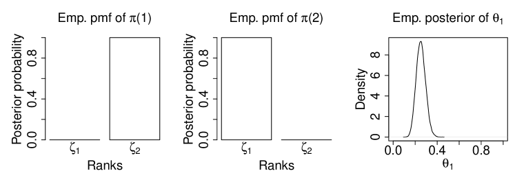
(b)

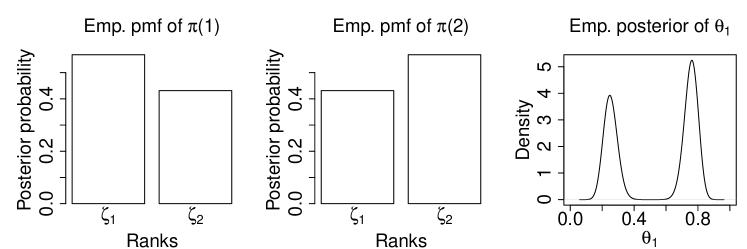
(c)

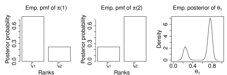
(d)

Figure 4: (a) True posterior marginals of all parameters. Empirical estimates of the marginal densities based on the DA chain with (b) 50 thousand iterations (c) 5 million iterations. (d) Empirical estimates of the marginal densities based on the sandwich chain with 50 thousand iterations.

(a)

(b)

Figure 5: Autocorrelation plots and trace plots for the DA and sandwich $\boldsymbol{\theta}$ chains ($\theta_{1}$ component) based on (a) 50 thousand iterations (trace plot shows last one thousand iterations) (b) 5 million iterations (trace plot shows 2,519,900 to 2,520,899 iterations).

Figure 6: The Gelman-Rubin diagnostic plots for the DA chain based on 4 parallel runs of length 50,000 each. The starting values of multiple chains were selected near the global mode (left) and the local mode (middle) and from both modes.

5 Real data application

In this section we illustrate the methods proposed in this article by applying them to a sushi preference data, previously published in the literature. The sushi preference data collected by Kamishima (2003) consists of complete rankings of few types of sushis by 5,000 respondents together with demographic data on the respondents. This dataset has also been used by Kamishima and Akaho (2009) for model based clustering of orderings. In this article, we consider four types of fish sushis: Anago (sea eel), Maguro (tuna), Toro (fatty tuna) and Tekka Maki (tuna roll). We study the role of gender (male or female), age and geographic location (east or west Japan) of the respondents on ranking of these four types of sushis. The variable age is categorized into six categories: 15–19 years, 20–29 years, 30–39 years, 40–49 years, 50–59 years and 60 years or above. Thus the respondents are categorized into overall 24 categories. Although Toro (fatty tuna) stands out as the most preferred sushi in all categories, substantial variability is observed in ranking the remaining three sushis. Thus apart from identifying the central ranking for these categories we are also interested in the heterogeneity in ranking of Anago, Maguro and Tekka Maki conditional on the Toro being the most preferred sushi. The MCMC sampling outputs allow us to compute these conditional probabilities without having to sum over an enormous $24^{24}$ dimensional joint distribution.

To this end, we ran our sandwich algorithm for a total of 60,000 iterations and discarded the first 10,000 iterations as burnins, although convergence was observed within first 15,000 iterations. As far as the marginal probabilities are concerned, the central ranks are same for all the categories and it is

Toro $\succ$ Maguro $\succ$ Tekka Maki $\succ$ Anago

where Toro $\succ$ Maguro means Toro is preferred to Maguro. However, there is substantial heterogeneity in ranking. The marginal probability that Toro is the most preferred sushi ranges from 66% to 69% except for females of age 60 years or more and currently living in west Japan, where the probability is 44.3%. However, the sample sizes are relatively small in these two categories – there are only 12 females in the east Japan of age 60 or above and only 5 females in the west of age 60 or above. Thus the marginal posterior distributions of the central ranks for these two categories have higher variability than the other groups. The joint (posterior) probability of Toro being the most favorite sushi across all the categories is 37% (se 0.2%). We calculate the Monte Carlo standard errors for the posterior estimates using batch means method (Flegal and Jones,, 2010). The joint (posterior) probability of Toro being among the top two favorite sushis across all the categories is 78% (se 0.3%). Thus Toro can be regarded as the most preferred sushi among the four.

Next assuming Toro being the most preferred, we compute the conditional probabilities of other sushis being the second most favorite in each of the groups. These conditional probabilities are highest for Maguro (tuna) and varies from 49% to 52% among the categories, followed by Anago (sea eel) with probabilities varying from 24% to 35%. The probability of Maguro being the second most favorite across all categories given that the Toro is the most favorite across all categories is 47% while the same probability for Anago is only 26%.

In order to judge any interaction effect present we compute the probability that the Toro is the most favorite sushi across all the age groups for each combination of gender (male/female) and geographic location (east/west). The solid lines in Figure 7 display these posterior probabilities for males (triangles) and females (circles). Notice that the posterior probability of Toro being the most favorite sushi among men does not change from east to west Japan but for women it does. Similarly we compute the posterior interaction probabilities for Maguro being the second most favorite conditional on Toro being the most favorite. The dashed lines in Figure 7 display these probabilities. Similar to the previous case, the conditional posterior probability changes for women from east to west Japan. However, this change is not as large as the previous case. Such interaction effects were found to be absent between age and gender, suggesting that the preferences towards different sushis do not, as such, depend on age.

Figure 7:

Interaction probabilities: the solid lines join the points denoting the posterior probabilities of Toro being the most favorite sushi across all age groups. The dashed lines join the points denoting the posterior probabilities of Maguro being the second most favorite sushi conditional on Toro being the most favorite across all age groups.

The variability in ranking is also reaffirmed by the small value of $\widehat{\lambda}=0.175$ (se 0.235) and the multi-modal posterior distribution of $\theta_{i}$’s. For example, the posterior density estimate of $\theta_{1}$ is shown in the left panel of Figure 8. It is important to note that exploring this variability in ranking is possible because our sandwich algorithm for $\boldsymbol{\theta}$ mixes very well (see right panel of Figure 8) and discovers all the modes of the posterior distributions of $\theta_{i}$’s.

Figure 8: Left: Multimodal posterior density of $\theta_{1}$. Right: Autocorrelation plots of the $\theta_{i}$ chains after thinning by 5.

6 Discussions

In comparison to the multinomial logit model, the new rank-data model presented in this paper is far more parsimonious and it requires estimation of far less number of parameters. In addition, the new rank-data model allows us to introduce a notion of central ranking that facilitates a natural modeling of the observed rank data as perturbations of the central rank. In the presence of categorical covariates the central rank may vary across categories and the rank-data model has been extended to incorporate this. While the estimation of the parameters of this new rank-data model is conceptually straight forward in a Bayesian set-up, considerable computational challenges are encountered due to the very slow convergence of the Gibbs sampler. Widely used diagnostics for detecting the convergence of the Gibbs sampler seem to fail in this situation. A new sandwich algorithm is devised for efficient posterior computation and is seen to perform effectively in the practically important situation when the number of items to be ranked is small. The case when one or more covariates are continuous will require development of a different technique and will be taken up in a future paper. We are also going to apply the proposed model and the MCMC algorithms in the context of partial rank data, that is, when not all available items are ranked.

7 Supplementary materials

The online supplementary materials contain codes for analyzing the sushi data.

Appendices

Appendix A Standard errors of $\hat{\lambda}$

To obtain the standard error of $\hat{\lambda},$ note that the negative of the observed information for $\lambda$ is given by

$$-I(\lambda|\textbf{y})=\frac{d^{2}}{d\lambda^{2}}\log c_{\lambda}(\textbf{y})$$

$$=\mathrm{E}~{}\left(\frac{d^{2}}{d\lambda^{2}}\log p(\textbf{y},\boldsymbol{\theta},\boldsymbol{\pi}|\lambda)\bigg{|}~{}\lambda\right)+\mathrm{Var}\left(\frac{d}{d\lambda}\log p(\textbf{y},\boldsymbol{\theta},\boldsymbol{\pi}|\lambda)\bigg{|}~{}\lambda\right)$$

$$=\mathrm{E}~{}\left(\frac{d^{2}}{d\lambda^{2}}\log p(\boldsymbol{\theta}|\lambda)\bigg{|}~{}\lambda\right)+\mathrm{Var}\left(\frac{d}{d\lambda}\log p(\boldsymbol{\theta}|\lambda)\bigg{|}~{}\lambda\right)$$

$$=\sum_{i=1}^{p!}|\zeta_{i}|^{2}e^{\lambda|\zeta_{i}|}\left\{\mathrm{E}(\log\theta_{i}|\textbf{y},\lambda)-\Psi_{1}\left(e^{\lambda|\zeta_{i}|}\right)e^{\lambda|\zeta_{i}|}-\Psi\left(e^{\lambda|\zeta_{i}|}\right)\right\}$$

$$\qquad+\Psi_{1}\left(\sum_{i=1}^{p!}e^{\lambda|\zeta_{i}|}\right)\left(\sum_{i=1}^{p!}e^{\lambda|\zeta_{i}|}\right)^{2}+\Psi\left(\sum_{i=1}^{p!}e^{\lambda|\zeta_{i}|}\right)\sum_{i=1}^{p!}e^{\lambda|\zeta_{i}|}$$

$$\qquad+\mathrm{Var}\left(\sum_{i=1}^{p!}|\zeta_{i}|e^{\lambda|\zeta_{i}|}\log\theta_{i}~{}\bigg{|}~{}\textbf{y},\lambda\right),$$

where the first equality follows from (Casella, 2001, p. 497), the second equality follows from Figure 1, and $\Psi(\cdot)$ and $\Psi_{1}(\cdot)$ are the digamma and the trigamma functions respectively. In the above, we approximate the conditional expectation and variance terms by the corresponding MCMC estimate using our sandwich chain. Consequently, the standard error of $\hat{\lambda}$ is given by s.e.$(\hat{\lambda})=I(\hat{\lambda}|\textbf{y})^{-1/2}$.

Appendix B The Mtm $K_{\boldsymbol{\pi}}$ when $p=2,g=2$

In order to write down the Mtm $K_{\boldsymbol{\pi}}$ of the DA chain $\{\boldsymbol{\pi}^{(m)}\}_{m\geq 0}$, we need to introduce some notations. Let $n_{ij}$ denote the number of observations in the $j$th category with rank $\zeta_{i}$ for $i,j=1,2$. Let $n_{i.}=n_{i1}+n_{i2}$ for $i=1,2$, $n_{d}=n_{11}+n_{22}$, and $n_{od}=n_{12}+n_{21}$. Let $r(x)=1/[x^{n_{1.}}(1-x)^{n_{2.}}+x^{n_{2.}}(1-x)^{n_{1.}}+x^{n_{d}}(1-x)^{n_{od}}+x^{n_{od}}(1-x)^{n_{d}}]$, $a=1/\mbox{Beta}(n_{1.}+a_{1},n_{2.}+a_{2})$, $b=1/\mbox{Beta}(n_{d}+a_{1},n_{od}+a_{2})$, $c=1/\mbox{Beta}(n_{od}+a_{1},n_{d}+a_{2})$, and $d=1/\mbox{Beta}(n_{2.}+a_{1},n_{1.}+a_{2})$. Let $k_{ij}$ be the $(i,j)$th element of the matrix $K_{\boldsymbol{\pi}}$, $i,j=1,2,3,4$. Then straightforward calculations show that

$$k_{11}=a\int_{0}^{1}r(x)x^{2n_{1.}+a_{1}-1}(1-x)^{2n_{2.}+a_{2}-1}dx$$

$$k_{12}=a\int_{0}^{1}r(x)x^{n_{1.}+n_{d}+a_{1}-1}(1-x)^{n_{2.}+n_{od}+a_{2}-1}dx$$

$$k_{13}=a\int_{0}^{1}r(x)x^{n_{1.}+n_{od}+a_{1}-1}(1-x)^{n_{2.}+n_{d}+a_{2}-1}dx$$

$$k_{14}=a\int_{0}^{1}r(x)x^{n+a_{1}-1}(1-x)^{n+a_{2}-1}dx$$

$$k_{21}=b\int_{0}^{1}r(x)x^{n_{1.}+n_{d}+a_{1}-1}(1-x)^{n_{2.}+n_{od}+a_{2}-1}dx$$

$$k_{22}=b\int_{0}^{1}r(x)x^{2n_{d}+a_{1}-1}(1-x)^{2n_{od}+a_{2}-1}dx$$

$$k_{23}=b\int_{0}^{1}r(x)x^{n+a_{1}-1}(1-x)^{n+a_{2}-1}dx$$

$$k_{24}=b\int_{0}^{1}r(x)x^{n_{2.}+n_{d}+a_{1}-1}(1-x)^{n_{1.}+n_{od}+a_{2}-1}dx$$

$$k_{31}=c\int_{0}^{1}r(x)x^{n_{1.}+n_{od}+a_{1}-1}(1-x)^{n_{2.}+n_{d}+a_{2}-1}dx$$

$$k_{32}=c\int_{0}^{1}r(x)x^{n+a_{1}-1}(1-x)^{n+a_{2}-1}dx$$

$$k_{33}=c\int_{0}^{1}r(x)x^{2n_{od}+a_{1}-1}(1-x)^{2n_{d}+a_{2}-1}dx$$

$$k_{34}=c\int_{0}^{1}r(x)x^{n_{2.}+n_{od}+a_{1}-1}(1-x)^{n_{1.}+n_{d}+a_{2}-1}dx$$

and finally

$$k_{41}=d\int_{0}^{1}r(x)x^{n+a_{1}-1}(1-x)^{n+a_{2}-1}dx$$

$$k_{42}=d\int_{0}^{1}r(x)x^{n_{d}+n_{2.}+a_{1}-1}(1-x)^{n_{od}+n_{1.}+a_{2}-1}dx$$

$$k_{43}=d\int_{0}^{1}r(x)x^{n_{2.}+n_{od}+a_{1}-1}(1-x)^{n_{1.}+n_{d}+a_{2}-1}dx$$

$$k_{44}=d\int_{0}^{1}r(x)x^{2n_{2.}+a_{1}-1}(1-x)^{2n_{1.}+a_{2}-1}dx.$$

As mentioned before, here we have ordered the points in the state space as follows: $(\zeta_{1},\zeta_{1})$, $(\zeta_{1},\zeta_{2})$, $(\zeta_{2},\zeta_{1})$, and $(\zeta_{2},\zeta_{2})$. So, for example, the element $k_{23}$ is the probability of moving from $(\zeta_{1},\zeta_{2})$ to $(\zeta_{2},\zeta_{1})$. Note that all of the transition probabilities are strictly positive, which implies that the DA chain is Harris ergodic.

References

- Brémaud (1999) Brémaud, P. (1999), Markov Chains Gibbs Fields, Monte Carlo Simulation, and Queues. Springer-Verlag, New York
- Brook and Upton (1974) Brook, D. and Upton, G. J. G. (1974) Biases in Local Government Elections Due to Position on the Ballot Paper. Applied Statistics, 23:414–419(6)
- Brown (1974) Brown, J.(1974) Recognition assessed by rating and ranking. British Journal of Psychology, 65,13–22
- Casella (2001) Casella, G. (2001) Empirical Bayes Gibbs sampling. Biostatistics, 2, 485–500.
- Cayley (1849) Cayley, A. (1849). Lxxvii. Note on the theory of permutations. The London, Edinburgh, and Dublin Philosophical Magazine and Journal of Science, 34, 527–529.
- Critchlow (1980) Critchlow, D. (1980) Metric methods for analyzing partially rank data. New York: Springer Verlag.
- Daniels (1950) Daniels, H. E. (1950) Rank correlation and population models. Biometrika, 33, 129-135.
- Diaconis (1988) Diaconis, P. (1988) Group representation in probability and statistics. Institute of Mathematical Statistics, Lecture Notes-Monograph Series, vol. 11.
- Diaconis (1989) Diaconis, P. (1989) A generalization of spectral analysis with application to ranked data. The Annals of Statistics, 17, 949-979
- Feigin and Cohen (1978) Feigin, P. and Cohen, A. (1978) On a model of concordance between judges. Journal of the Royal Statistical Society, Series B, 40, 203-213.
- Flegal and Jones, (2010) Flegal, J. M. and Jones, G. L. (2010). Batch means and spectral variance estimators in Markov chain Monte Carlo. Ann. Statist., 38:1034–1070.
- Fligner and Verducci (1986) Fligner, M. A. and Verducci, J. S. (1986) Distance based ranking models. Journal of the Royal Statistical Society, Series B, 48, 359-369.
- Fligner and Verducci (1988) Fligner, M. A. and Verducci, J. S. (1988) Multistage ranking models. Journal of the American Statistical Association, 83, 892-901.
- Frühwirth-Schnatter, S. (2001) Frühwirth-Schnatter, S. (2001). Markov chain Monte Carlo estimation of classical and dynamic switching and mixture models. Journal of the American Statistical Association, 96:194–209.
- Gelman and Rubin (1992) Gelman, A. and Rubin, D. B. (1992) Inference from iterative simulation using multiple sequences. Statistical Science, 7, 457-472
- Gormley and Murphy (2008) Gormley, I. C. and Murphy, T. B. (2008) A mixture of experts model for rank data with applications in election studies. The Annals of Applied Statistics, 2, 1452–1477.
- Gormley and Murphy (2010) Gormley, I. C. and Murphy, T. B. (2010) A mixture of experts latent position cluster model for social network data. Statistical Methodology, 7, 385–405
- Hobert and Marchev (2008) Hobert, J. P. and Marchev, D. (2008) A theoretical comparison of the data augmentation, marginal augmentation and PX-DA algorithms. The Annals of Statistics, 36, 532-554
- Hobert, Roy and Robert (2011) Hobert, J. P. and Roy, V. and Robert, C. P. (2011) Improving the convergence properties of the data augmentation algorithm with an application to Bayesian mixture modelling. Statistical Science, 26, 332-351
- Kamishima (2003) Kamishima, T. (2003). Nantonac collaborative filtering: recommendation based on order responses.In Proceedings of the Ninth ACM SIGKDD International Conference on Knowledge Discovery and Data Mining, pp. 583–588. ACM.
- Kamishima and Akaho (2009) Kamishima, T. and Akaho, S. (2009). Efficient Clustering for Orders. In Mining Complex Data, Vol.165 of Studies in Computational Intelligence, D. A. Zighed, S. Tsumoto, Z. W. Ras, and H. Hacid, eds,, Chapter 15, pp. 261–280.
- Laha and Dongaonkar (2009) Laha, A. K. and Dongaonkar, S. (2009) Bayesian Analysis of Rank Data using SIR. In Advances in Multivariate Statistical Methods. Sengupta, A. (Ed.). World Scientific Publshers
- Lebanon and Lafferty (2002) Lebanon, G. and Lafferty, J. (2002) Cranking: Combining rankings using conditional probability models on permutations. In Proceedings of the 19th international conference on machine learning, Morgan Kaufmann, San Francisco USA, 363-370
- Liu, Wong and Kong (1994) Liu, J. S. and Wong, W. H. and Kong, A. (1994) Covariance Structure of the Gibbs Sampler with Applications to Comparisons of Estimators and Augmentation Schemes. Biometrika, 81 , 27-40
- Liu and Wu (1999) Liu, J. S. and Wu, Y. N. (1999) Parameter Expansion for Data Augmentation. Journal of the American Statistical Association 94, 1264-1274
- Mallows (1957) Mallows, C. L. (1957) Non-null ranking models. Biometrika, 44, 114-130.
- McCullagh (2011) McCullagh, P. (2011) Random permutations and partition models. In International Encyclopedia of Statistical Science, Springer Berlin Heidelberg, 1170–1177
- Meng and van Dyk (1999) Meng, X.-L. and van Dyk, D. A. (1999) Seeking Efficient Data Augmentation Schemes via Conditional and Marginal Augmentation. Biometrika, 86, 301-320
- Meyn and Tweedie (1993) Meyn, S. P. and Tweedie, R. L. (1993) Markov Chains and Stochastic Stability. Springer Verlag, London
- Mosteller (1951) Mosteller, F. (1951) Remarks on the method of paired comparisons: I. The least squares solution assuming equal standard deviations and equal correlations. Psychometrika, 16, 3-9.
- Murphy and Martin (2003) Murphy, T. B. and Martin, D. (2003) Mixtures of distance-based models for ranking data. Computational Statistics and Data Analysis, 41, 645-655.
- Robert and Casella (2004) Robert C. P. and Casella, G. (2004) Monte Carlo Statistical Methods, 2nd edn. Springer, New York (2004)
- Roy (2012a) Roy, V. (2012) Spectral analytic comparisons for data augmentation. Statistics and Probability Letters, 82, 103-108
- Roy (2012b) Roy, V. (2012) Convergence rates for MCMC algorithms for a robust Bayesian binary regression model. Electronic Journal of Statistics, 6, 2463–2485
- Roy (2014) Roy, V. (2014) Efficient estimation of the link function parameter in a robust Bayesian binary regression model. Computational Statistics and Data Analysis, 73, 87–102.
- Roy and Hobert (2007) Roy, V. and Hobert, J. P. (2007) Convergence rates and asymptotic standard errors for MCMC algorithms for Bayesian probit regression. Journal of the Royal Statistical Society, Series B, 69, 607-623
- Russell and Gray (1994) Russell, P. A. and Gray, C. D. (1994) Ranking or rating? Some data and their implications for the measurement of evaluative response. British Journal of Psychology, 85, 79–92
- Thurstone (1927) Thurstone, L. L. (1927) A law of comparative judgment. Psychological Review, 79, 281-299.
- Yellot (1977) Yellot, J. (1977) The relationship between Luce’s choice axiom, Thurstone theory of comaparative judgment, and the double exponential distribution. Journal of Mathematical Psychology, 15,109-144.
- Yu (2000) Yu, Philip L. H. (2000) Bayesian analysis of order-statistics models for ranking data. Psychometrika, 65, 281-299.
- Yu and Meng (2011) Yu, Y. and Meng, X.-L. (2011) To center or not to center: that is not the question - An ancillarity-sufficiency interweaving strategy (ASIS) for boosting MCMC efficiency. Journal of Computational and Graphical Statistics 20, 531-570