Graph Classification via Deep Learning with Virtual Nodes

Abstract

Learning representation for graph classification turns a variable-size graph into a fixed-size vector (or matrix). Such a representation works nicely with algebraic manipulations. Here we introduce a simple method to augment an attributed graph with a virtual node that is bidirectionally connected to all existing nodes. The virtual node represents the latent aspects of the graph, which are not immediately available from the attributes and local connectivity structures. The expanded graph is then put through any node representation method. The representation of the virtual node is then the representation of the entire graph. In this paper, we use the recently introduced Column Network for the expanded graph, resulting in a new end-to-end graph classification model dubbed Virtual Column Network (VCN). The model is validated on two tasks: (i) predicting bio-activity of chemical compounds, and (ii) finding software vulnerability from source code. Results demonstrate that VCN is competitive against well-established rivals.

1 Intro

Deep learning has achieved record-breaking successes in domains with regular grid (e.g., via CNN) or chain-like (e.g., via RNN) structures LeCun et al. (2015). However, many, if not most, real-world structured problems are best modelled using graphs with irregular connectivity. These include, for example, chemical compounds, proteins, RNAs, function calls in software, brain activity networks, and social networks. A canonical task is graph classification, that is, assigning class labels to a graph instance (e.g., chemical compound as its activity against cancer cells).

We study a generic class known as attributed graphs whose nodes can have attributes, and edges can be multi-typed and directed. We aim to efficiently learn distributed representation of graph, that is, a map that turns variable-size graphs into fixed-size vectors or matrices. Such a representation would benefit greatly from a powerful pool of data manipulation tools. This rules out traditional approaches such as graph kernels Vishwanathan et al. (2010) and graph feature engineering Choetkiertikul et al. (2017), which could be either computation or labor intensive.

Several recent neural networks defined on graphs, such as Graph Neural Network Scarselli et al. (2009), diffusion-CNN Atwood and Towsley (2016), and Column Network Pham et al. (2017a), start with node representations by taking into account of the neighborhood structures, typically through convolution and/or recurrent operations. Node representations can then be aggregated into graph representation. It is akin to representing a document by first embedding words into vectors (e.g., through word2vec) then combining them (e.g., by weighted averaging using attention). We conjecture that a better way is to learn graph representation directly and simultaneously with node representation.

Our main idea is to augment the original graph with a virtual node to represent the latent aspects of the graph. The virtual node is bidirectionally connected to all existing real nodes. The virtual node assumes either empty attributes or auxiliary information which are not readily available in the original graph. The augmented-graph is passed through the existing graph neural networks for computing node representation. The graph representation is then a vector representation of the virtual node.

For concreteness, we materialize the idea of virtual node using Column Network Pham et al. (2017a), an architecture for node classification. With a differentiable classifier (e.g., a feedforward net), the network is an end-to-end solution for graph classification, which we name Virtual Column Network (VCN). We validate the VCN on two applications: predicting bio-activity of chemical compounds, and assessing vulnerability in software code and the results are promising.

2 Models

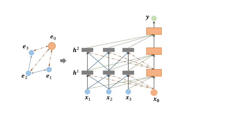
Figure 1: Virtual Column Network (VCN) = Column Network + Virtual Node. (Left) A graph of 3 nodes augmented with a virtual node $\boldsymbol{e}_{0}$ connecting to all nodes. (Right) The VCN model for the graph, where $\boldsymbol{x}_{0}$ is vector of graph descriptors (if any), $\boldsymbol{x}_{1},\boldsymbol{x}_{2},\boldsymbol{x}_{3}$ are node attributes, and $y$ is the graph label. Boxes are hidden layers.

In this section we present Virtual Column Network (VCN), a realization of the idea of virtual node for graph classification using a recent node representation method known as Column Network (CLN) Pham et al. (2017a). VCN is applicable to graphs of multi-typed edges and attributed nodes.

2.1 Column Network

Given a attributed graph, Column Network is a recurrent neural architecture defined on it. For each network, there are multiple interacting recurrent nets (called columns, as analogy to cortical columns in brain Mountcastle (1997)), each of which is responsible to a node. Fig. 1 illustrates the VCN model, where the columns of $\boldsymbol{x}_{1},\boldsymbol{x}_{2},\boldsymbol{x}_{3}$ create a Column Network. Neural connections from one column to another reflect the graph edge between the two corresponding nodes. More concretely, the column for node $i$ ($i=1,...n$) at step $t$ is updated using information from neighbors at step $t-1$ as follows:

$$\boldsymbol{c}_{ip}^{t} =\frac{1}{\mid N_{p}\left(i\right)\mid}\sum_{j\in N_{p}\left(i\right)}\boldsymbol{h}_{j}^{t-1}$$

$$\tilde{\boldsymbol{h}}_{i}^{t} =g\left(W\boldsymbol{h}_{i}^{t-1}+\sum_{p}U_{p}\boldsymbol{c}_{ip}^{t}\right)$$

$$\boldsymbol{h}_{i}^{t} =(1-\boldsymbol{\alpha}_{i}^{t})\ast\boldsymbol{h}_{i}^{t-1}+\boldsymbol{\alpha}_{i}^{t}\ast\tilde{\boldsymbol{h}}_{i}^{t}$$

where:

• $\boldsymbol{h}_{i}^{t}$ denotes the state of column $i$ at step $t$;

• $N_{p}\left(i\right)$ is the neighborhood of node $i$ w.r.t. edge type $p$;

• $\boldsymbol{c}_{ip}^{t}$ denotes the neighboring context w.r.t. edge type $p$;

• $\tilde{\boldsymbol{h}}_{i}^{t}$ is the candidate state, and $g(\cdot)$ is nonlinear transformation (e.g., ReLU or tanh); $W_{i},U_{ip}$ are parameters tied across steps. When columns are homogeneous, we can have remove the sub-index $i$;

• $\boldsymbol{\alpha}_{i}^{t}\in(0,1)$ is the smoothing gate, which is parameterized in the same way as $\tilde{\boldsymbol{h}}_{i}^{t}$, and $g(\cdot)$ is typically a sigmoid function.

At $t=1$, the state is assigned to the projection of attributes at node $i$, i.e., $\boldsymbol{h}_{i}^{1}=P_{i}\boldsymbol{x}_{i}$.

Remark: $\boldsymbol{c}_{i}^{t}$ plays the role of usual input at step $t$ for RNN. Without this, the model becomes the Highway Network Srivastava et al. (2015) with parameters typing Pham et al. (2016). This also suggests a GRU alternative with a reset gate $\boldsymbol{r}_{i}^{t}\in(0,1)$, i.e., $\tilde{\boldsymbol{h}}_{i}^{t}=g\left(W\left(\boldsymbol{r}_{i}^{t}\ast\boldsymbol{h}_{i}^{t-1}\right)+\sum_{p}U_{p}\boldsymbol{c}_{ip}^{t}\right)$. When there is only one neighbor per type, computing the candidate $\tilde{\boldsymbol{h}}_{i}^{t}$ becomes the standard convolution operation in CNN with neighbor indexed by $p$. More specifically, $\boldsymbol{c}_{ip}^{t}=\boldsymbol{h}_{j}^{t-1}$ for $N_{p}\left(i\right)\equiv j$ , leading to $\tilde{\boldsymbol{h}}_{i}^{t}=g\left(W\boldsymbol{h}_{i}^{t-1}+\sum_{j=N_{p}\left(i\right)}U_{p}\boldsymbol{h}_{j}^{t-1}\right)$.

2.2 Virtual Columns

Column networks are compact and effective in integrating long-range dependencies between nodes (the radius is equal to the height of the columns). However, it was designed for node classification. For graph classification we need a way to pool node states. A simple way is taking an average at the end: $\bar{\boldsymbol{h}}=\frac{1}{n}\sum_{i}\boldsymbol{h}_{i}^{T}$.

Here we introduce a new way for integrating node states. In particular, we augment a virtual node to the original graph bidirectionally connecting to all real nodes (See Fig. 1 for illustration). The corresponding virtual column hence performs two functions: (i) integrating state information from all node columns, and (ii) distributing the consensus graph-level information to all node columns. The virtual column can optionally take graph-level information as input (e.g., graph descriptors that are not encoded in the graph structure).

With the virtual column, high-order and implicit dependencies are distributed much faster, taking only 2 steps, independent of the graph size. The virtual column and the node columns are computed as follow:

$$\boldsymbol{h}_{0}^{t} = g\left(W_{0}\boldsymbol{h}_{0}^{t-1}+\frac{1}{n}\sum_{i=1}^{n}U_{0}\boldsymbol{h}_{i}^{t-1}\right)$$

$$\boldsymbol{h}_{i}^{t} = g\left(W\boldsymbol{h}_{i}^{t-1}+V\boldsymbol{h}_{0}^{t-1}+\sum_{p}U_{p}\boldsymbol{c}_{ip}^{t}\right)$$

Let $\boldsymbol{h}_{0}^{T}$ be the state of the virtual column at step $T$. The iterative estimation can continue (a) with dimensional change, which requires a projection onto a different state space, (b) without input from other nodes. The later part of the column is essentially a Highway Network Srivastava et al. (2015) with parameters typing Pham et al. (2016) (or a GRU if a reset gate is used Li et al. (2016)).

Remark: In a way, it is similar to semi-restricted Boltzmann machines, where the real columns and their connections handle short-range dependencies, and the virtual column enables long-range dependencies. The recurrent structure is akin to mean-field unrolled to $T$ steps.

3 Experiments

We demonstrate the effectiveness of our model against the baselines on BioAssay activity prediction tasks and a code classification task.

3.1 Experiment settings

For all experiments with our proposed VCN, we use Highway network for all layers and ReLU as activation function. Dropout Srivastava et al. (2014) is applied before and after the column layers. Each dataset is divided into training, validation and test sets. The validation set is used for early stopping and tuning hyper-parameters. We set the number of hidden layers by 10, the mini-batch by 100 and search for (i) hidden dimensions of the virtual columns, (ii) the hidden dimensions of the node columns, (iii) the learning rate $\eta$ (0.001, 0.002,…,0.005) and (iv) optimizers: Adam Kingma and Ba (2014) or RMSprop. The training starts at the learning rate $\eta$ and will be divided by 2 if the model cannot find a better result on the validation set. Learning is terminated after 4 times of halving or after 500 epochs. The best setting is chosen by the validation set and the result of the test set are reported.

Baselines are SVM, Random Forest and Gradient Boosting Machine. These method reads input as vector representation of graphs. Sec. 3.2.2 and Sec. 3.3.2 describe feature extraction methods for the baselines. For BioAssay activity prediction, we add Neural Fingerprint (NeuralFP) Duvenaud et al. (2015) as a baseline.

3.2 BioAssay Activity Prediction

3.2.1 Datasets

The first set of experiments uses 3 largest NCI BioAssay activity tests collected from the PubChem website : Lung Cancer, Leukemia and Yeast Anticancer. Each BioAssay test contains records of activities for chemical compounds. Each compound is represented as a graph, where nodes are atoms and edges are bonds between them. We chose the 2 most common activities for classification: “active” and “inactive”. The statistics of data is reported in Table 1. These datasets are unbalanced, therefore “inactive” compounds are randomly removed so that each of Lung Cancer and Leukemia datasets has 10,000 graphs and the Yeast Anticancer dataset has 25,000 graphs.

No.	Dataset	# Active	# Graph
1	Lung Cancer	3,026	38,588
2	Leukemia	3,681	38,933
3	Yeast Anticancer	10,090	86,130

Table 1: Summary of the three NCI BioAssay datasets. “# Graph” is the number of graphs and “# Active” is the number of active graph against a BioAssay test.

3.2.2 Feature extraction

We use RDKit toolkit for molecular feature extraction . RDKit computes fixed-dimensional feature vectors of molecules, which is so-called circular fingerprint. These vectors are used as inputs for the baselines. We set the dimension of the fingerprint features by 1024.

For our model, we also use RDKit to extract the structure of molecules and the atom features. An atom feature vector is the concatenation of the one-hot vector of the atom and other features such as atom degree and number of H atoms attached. We also make use of bond features such as bond type and a binary value indicating if a bond in a ring.

3.2.3 Results

Table 2 reports results, measured in AUC, on the NCI datasets. The proposed Virtual Column Network (VCN) is competitive against best feature engineering techniques (cicular fingerprint and high-performing classifiers).

Method	Lung	Leukemia	Yeast	Average
FP+SVM	85.1	82.1	77.3	81.5
FP+RF	85.2	82.1	76.5	81.3
FP+GBM	81.5	82.3	77.0	80.3
NeuralFP	85.5	84.5	79.5	83.2
VCN	86.3	83.3	81.1	83.6

Table 2: Area under the ROC curve (AUC) (%) for NCI datasets. FP = Fingerprint; RF = Random Forests; GBM = Gradient Boosting Machine; VCN = proposed Virtual Column Network.

Fig. 2 reports the F1-score on the NCI datasets. On average, VCN beats all the baselines.

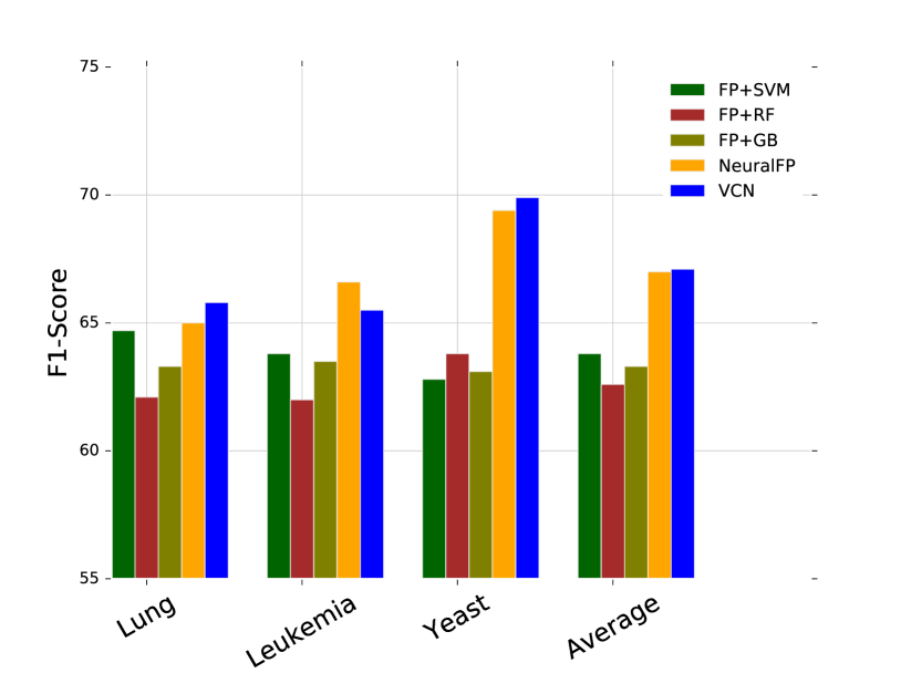
Figure 2: F1-score (%) for NCI datasets. FP = Fingerprint; RF = Random Forests; GBM = Gradient Boosting Machine; VCN = proposed Virtual Column Network. Best view in color.

3.3 Code Classification

3.3.1 Dataset

The dataset contains 18 Java projects, each consists of a number of source code files. Each source file is a Java class, which has a list attribute declarations and a number of methods. A class is represented as a graph, where graph-level features are the attribute declarations, nodes are methods and edges are method call. The task is to predict if a source file is vulnerable. The dataset is pre-processed by removing all replicated files of different versions in the same projects. This remains 2836 samples in total and 1020 positive ones.

3.3.2 Feature extraction

Methods and attribute declarations of Java classes can be considered as sequences of tokens and their representation can be learned through language modeling using LSTM Hochreiter and Schmidhuber (1997) with Noise Contrastive Estimation (NCE) Mnih and Teh (2012). The feature vector of each sequence is the mean of all hidden states outputted by the LSTM. After this step, each sequence is represented as a feature vector of 128 units. For the baselines, the feature vector of each Java class is the mean of feature vectors of all methods and attribute declarations. For the VCN model, the feature vector of the attribute declarations is the input for the virtual column.

3.3.3 Results

Fig. 3 reports the performance on Code classification task in AUC and F1-score. VCN outperforms all the baselines on both measures.

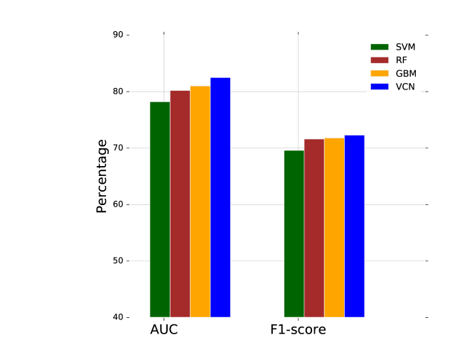
Figure 3: Performance on Code classification dataset, measured in AUC and F1-score (%).

4 Related Work

There has been a sizable rise of learning graph representation in the past few years Bronstein et al. (2016); Bruna et al. (2014); Henaff et al. (2015); Johnson (2017); Li et al. (2016); Niepert et al. (2016); Schlichtkrull et al. (2017). A number of works derive shallow embedding methods such as node2vec and subgraph2vec, possibly inspired by the success of embedding in linear-chain text (word2vec and paragraph2vec). Deep spectral methods have been introduced for graphs of a given adjacency matrix Bruna et al. (2014), whereas we allow arbitrary graph structures, one per graph. Several other methods extend convolutional operations to irregular local neighborhoods Atwood and Towsley (2016); Niepert et al. (2016); Pham et al. (2017a). Yet recurrent nets are also employed along the random walk from a node Scarselli et al. (2009).

This paper is built upon our recent work, the Column Network (real nodes only, designed for node classification) Pham et al. (2017a), and Column Bundle (no graphs, designed for multi-part data, where part can be instance or view) Pham et al. (2017b). Like is predecessors, it can be seen as an instance of learning as iterative estimation Greff et al. (2017).

Our application to chemical compound classification bears some similarity to the work of Duvenaud et al. (2015), where graph embedding is also collected from node embedding at each layer and refined iteratively from the bottom to the top layers. However, our treatment is more principled and more widely applicable to multi-typed edges.

5 Discussion

We have proposed a simple solution for learning representation of a graph: adding a virtual node to the existing graph. The expanded graph can then be passed through any node representation method, and the representation of the virtual node is the graph’s. The virtual node, coupled with a recent node representation method known as Column Network Pham et al. (2017a), results in a new graph classification method called Virtual Column Network (VCN). We demonstrate the power of the VCN on two tasks: (i) classification of bio-activity of chemical compounds against a given cancer; (ii) detecting software vulnerability from source code. Overall, the automatic representation learning is more powerful than state-of-the art feature engineering.

There are rooms open for further investigations. First, we can use multiple virtual nodes instead of just one.The graph is then embedded into a matrix whose columns are vector representation of virtual nodes. This will be beneficial in several ways. For multitask learning, each virtual node will be used for a task and all tasks share the same node representations. For big graphs with tight subgraph structures, each virtual node can target a subgraph. Second, other node representation architectures beside Column Networks are also applicable for deriving graph representation, including Gated Graph Sequence Neural Network Li et al. (2016), Graph Neural Network Scarselli et al. (2009) and diffusion-CNN Atwood and Towsley (2016).

Acknowledgments

The paper is partly supported by the Samsung 2016 GRO Program titled “Predicting hazardous software components using deep learning”, and the Telstra-Deakin CoE in Big Data and Machine Learning.

References

- Atwood and Towsley [2016] James Atwood and Don Towsley. Diffusion-convolutional neural networks. In Advances in Neural Information Processing Systems, pages 1993–2001, 2016.
- Bronstein et al. [2016] Michael M Bronstein, Joan Bruna, Yann LeCun, Arthur Szlam, and Pierre Vandergheynst. Geometric deep learning: going beyond euclidean data. arXiv preprint arXiv:1611.08097, 2016.
- Bruna et al. [2014] Joan Bruna, W Zaremba, A Szlam, and Yann LeCun. Spectral networks and deep locally connected networks on graphs. In ICLR, 2014.
- Choetkiertikul et al. [2017] Morakot Choetkiertikul, Hoa Khanh Dam, Truyen Tran, Aditya Ghose, and John Grundy. Predicting delivery capability in iterative software development. IEEE Transactions on Software Engineering, 2017.
- Duvenaud et al. [2015] David K Duvenaud, Dougal Maclaurin, Jorge Iparraguirre, Rafael Bombarell, Timothy Hirzel, Alán Aspuru-Guzik, and Ryan P Adams. Convolutional networks on graphs for learning molecular fingerprints. In Advances in neural information processing systems, pages 2224–2232, 2015.
- Greff et al. [2017] Klaus Greff, Rupesh K Srivastava, and Jürgen Schmidhuber. Highway and residual networks learn unrolled iterative estimation. ICLR, 2017.
- Henaff et al. [2015] Mikael Henaff, Joan Bruna, and Yann LeCun. Deep convolutional networks on graph-structured data. arXiv preprint arXiv:1506.05163, 2015.
- Hochreiter and Schmidhuber [1997] Sepp Hochreiter and Jürgen Schmidhuber. Long short-term memory. Neural computation, 9(8):1735–1780, 1997.
- Johnson [2017] Daniel D Johnson. Learning graphical state transitions. ICLR, 2017.
- Kingma and Ba [2014] Diederik Kingma and Jimmy Ba. Adam: A method for stochastic optimization. arXiv preprint arXiv:1412.6980, 2014.
- Le and Mikolov [2014] Quoc V Le and Tomas Mikolov. Distributed representations of sentences and documents. ICML, 2014.
- LeCun et al. [2015] Yann LeCun, Yoshua Bengio, and Geoffrey Hinton. Deep learning. Nature, 521(7553):436–444, 2015.
- Li et al. [2016] Yujia Li, Daniel Tarlow, Marc Brockschmidt, and Richard Zemel. Gated graph sequence neural networks. ICLR, 2016.
- Mnih and Teh [2012] Andriy Mnih and Yee Whye Teh. A fast and simple algorithm for training neural probabilistic language models. In In Proceedings of the International Conference on Machine Learning. Citeseer, 2012.
- Mountcastle [1997] Vernon B Mountcastle. The columnar organization of the neocortex. Brain, 120(4):701–722, 1997.
- Niepert et al. [2016] Mathias Niepert, Mohamed Ahmed, and Konstantin Kutzkov. Learning convolutional neural networks for graphs. In Proceedings of the 33rd annual international conference on machine learning. ACM, 2016.
- Pham et al. [2016] Trang Pham, Truyen Tran, Dinh Phung, and Svetha Venkatesh. Faster training of very deep networks via p-norm gates. ICPR, 2016.
- Pham et al. [2017a] Trang Pham, Truyen Tran, Dinh Phung, and Svetha Venkatesh. Column networks for collective classification. AAAI, 2017.
- Pham et al. [2017b] Trang Pham, Truyen Tran, and Svetha Venkatesh. One size fits many: Column bundle for multi-x learning. arXiv preprint arXiv:1702.07021, 2017.
- Scarselli et al. [2009] Franco Scarselli, Marco Gori, Ah Chung Tsoi, Markus Hagenbuchner, and Gabriele Monfardini. The graph neural network model. IEEE Transactions on Neural Networks, 20(1):61–80, 2009.
- Schlichtkrull et al. [2017] Michael Schlichtkrull, Thomas N Kipf, Peter Bloem, Rianne van den Berg, Ivan Titov, and Max Welling. Modeling relational data with graph convolutional networks. arXiv preprint arXiv:1703.06103, 2017.
- Srivastava et al. [2014] Nitish Srivastava, Geoffrey Hinton, Alex Krizhevsky, Ilya Sutskever, and Ruslan Salakhutdinov. Dropout: A simple way to prevent neural networks from overfitting. Journal of Machine Learning Research, 15:1929–1958, 2014.
- Srivastava et al. [2015] Rupesh K Srivastava, Klaus Greff, and Jürgen Schmidhuber. Training very deep networks. In Advances in neural information processing systems, pages 2377–2385, 2015.
- Vishwanathan et al. [2010] S Vichy N Vishwanathan, Nicol N Schraudolph, Risi Kondor, and Karsten M Borgwardt. Graph kernels. Journal of Machine Learning Research, 11(Apr):1201–1242, 2010.