Rogue waves and entropy consumption

Abstract

Based on data from the Japan Sea and the North Sea the occurrence of rogue waves is analyzed by a scale dependent stochastic approach, which interlinks fluctuations of waves for different spacings. With this approach we are able to determine a stochastic cascade process, which provides information of the general multipoint statistics. Furthermore the evolution of single trajectories in scale, which characterize wave height fluctuations in the surroundings of a chosen location, can be determined. The explicit knowledge of the stochastic process enables to assign entropy values to all wave events. We show that for these entropies the integral fluctuation theorem, a basic law of non-equilibrium thermodynamics, is valid. This implies that positive and negative entropy events must occur. Extreme events like rogue waves are characterized as negative entropy events. The statistics of these entropy fluctuations changes with the wave state, thus for the Japan Sea the statistics of the entropies has a more pronounced tail for negative entropy values, indicating a higher probability of rogue waves.

Oceanic rogue waves are usually defined as extremely large waves that occur suddenly and unexpectedly, even in situations where the ocean appears relatively calm and quiet Birkholz et al. (2015). While there are numerous reports from sailors claiming to have observed a rogue wave in the open ocean, rogue waves are very rare, which makes researching or forecasting difficult Soto-Crespo et al. (2016). Because of their size rogue waves can be extremely dangerous, even to the large ocean liners, appearing in different forms of rare large amplitude events Onorato et al. (2013). As a prototypical example of extreme events emerging in a stochastic “background”, rogue waves have been investigated from various perspectives, e.g. using tools from non-linear waves and soliton theory Chabchoub et al. (2011).

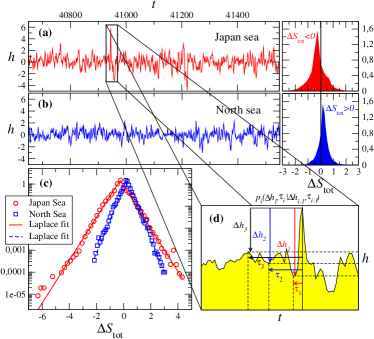
Figure 1: (a) Series of sea surface height taken at the Japan Sea, where rogue waves are observed, and (b) surface heights from the North Sea, where rogue waves are not observed. All heights are given in units of meter. On the right, one plots the distribution of entropies variations through trajectories associated to each series, which are well approximated by (c) the Laplace distribution, with negative median for Japan sea. (d) Illustration of the sea-level heights, as a scale process (see text).

Due to the scarcity of observational data, many fundamental questions are still under debate. What exactly causes a specific rogue wave? Are there any fundamental features of the ambient sea state that lead to the occurrence of a rogue wave in the ocean? Is it possible to provide quantitative insight into how probable it is to observe a rogue wave? Often investigations into rogue waves are based on models for wave packet evolution in non-linear dispersive media Onorato et al. (2013). Studies have been successful in demonstrating the existence of rogue waves and also allowed classifying them into different classes. Still, the approach is fundamentally deterministic, while, as the definition of rogue waves itself suggests, a probabilistic description seems more natural.

In this paper we provide what is, to our knowledge, the first evidence for thermodynamical processes underlying the occurrence of rogue waves in nature. Our findings do not contradict the findings from previous deterministic approaches to investigate rogue waves, but instead complement the present understanding with a thermostatistical perspective.

The findings reported here are based on the combination of two important features that rogue waves share with extreme events in general Hadjihosseini et al. (2014, 2016): first, they occur within short time-scales; second, their large amplitude variations reflect a flow of energy coming from the largest scales. This energy flow through scales underlying the occurrence of a rogue wave is similar to the picture of the energy flux in Kolmogorov’s turbulence cascade Kolmogorov (1941). Our work presents first evidence of a physical connection between the emergence of extreme events in systems far from equilibrium and the fundamental features of energy flow in them.

Two observational data sets are analyzed, one collected at the Japan Sea, where rogue waves are observed, and another collected at the North sea, where rogue waves are almost absent Mori et al. (2002); Mori and Yasuda (2002). Figures 1a and 1b sketch a part of these two observational series. The series from the Japan sea (Fig. 1a) includes the measured signal of one rogue wave with a height of about $6$ meters.

We will show that the structure of rogue waves results from an exchange of entropy between the wave environment and the local wave condition itself, along a trajectory “downscale”. Furthermore, the distribution of the total entropy variation along these downscale trajectories differ for the two cases: in the data set where rogue waves are absent it has a positive mode, whereas for the Japanese data set, which includes rogue waves, the distribution mode is negative. See the right plots of Figs. 1a and 1b and Fig. 1c.

For the proper analysis of the stochastic series in Fig. 1, one aims at the derivation of a predictor $h_{t+\tau}$ for the next time step $t+\tau$, based on past measurements of the series, $\{h_{t},h_{t-\tau},\dots,h_{t-N\tau}\}$. Here, $\tau$ is taken as the unitary time-lag between successive measurements. If the process is Markovian throughout its time evolution, the predictor is a function of the present state $h_{t}$ only, and the time series can be statistically reproduced using the $2$-point statistics $p(h_{t+\tau},h_{t})$. The propagator is then simply the conditional probability density function $p(h_{t+\tau}|h_{t})=p(h_{t+\tau},h_{t})/p(h_{t})$ with $p(h_{t})=\int p(h_{t+\tau},h_{t})dh_{t+\tau}$. When the process is not Markovian, each value in the series depends on a larger set of previous values and consequently one needs to extract a $N$-point statistics, for larger $N>2$, which, in practice, is very cumbersome and challenging. Ocean surface level time series turn out not to be Markovian.

It is possible to overcome this shortcoming if one considers the concept of “scale process”Nickelsen and Engel (2013); Seifert (2005, 2012), illustrated in Fig. 1d. A scale process describes how the variables’ increments $\Delta h_{k,t}:=h_{t}-h_{t-\tau_{k}}$ change with $\tau_{k}:=k\tau$ for a fixed time $t$ and a chosen value of $\tau$. Here we denote time-lags as time-scales. With such a concept, we now define the ensemble $\Delta h_{k,t}$ for fixed $t$ as a scale trajectory through time-scales $\tau_{k}$ ($k=1,\dots,N-1$).

To convert the series of sea-level height measurements in time to its scale or increment counterparts has profound consequences, as the latter now turns out to be Markovian Hadjihosseini et al. (2014, 2016). As a consequence the full analysis of the data, based on the computation of the $N$-point propagator $p(h_{t}|h_{t-\tau_{1}},...,h_{t-\tau_{N-1}})$ that predicts the time series of heights, can be decomposed into $N-2$ increment propagators $p(\Delta h_{k,t}|\Delta h_{k+1,t},h_{t})$ for each scale $k$ together with the initial distribution, $p(\Delta h_{0},\tau,h_{t})$ Hadjihosseini et al. (2016), see also supplementary material I.

Each increment propagator can be extracted separately from the time series Friedrich and Peinke (1997); Friedrich et al. (2011), defining a Fokker-Planck equationRisken (1984) for the respective time-scale,

$$-\tau\frac{\partial}{\partial\tau}p(\Delta h_{k}|\Delta h_{k^{\prime}},h)=$$ (1)

$$-\frac{\partial}{\partial\Delta h_{k}}\left[D^{(1)}(\Delta h_{k},h)p(\Delta h_{k}|\Delta h_{k^{\prime}},h)\right]$$

$$+\frac{\partial^{2}}{\partial\Delta h_{k}^{2}}\left[D^{(2)}(\Delta h_{k},h)p(\Delta h_{k}|\Delta h_{k^{\prime}},h)\right],$$

where the dependent variable is the height increment $\Delta h$ and the independent variables is the time-lag (time scale) $\tau_{k}$ or, respectively, $k$Friedrich et al. (2011). The surface elevation $h$ itself comes in as a second independent variable. This ensemble of Fokker-Planck equations is defined through the extraction of the corresponding family of drift and diffusion functions, $D^{(1)}(\Delta h_{k},\tau_{k},h)$ and $D^{(2)}(\Delta h_{k},\tau_{k},h)$, for the set of scales $k$ asRisken (1984)

$$D^{(n)}(\Delta h_{k},\tau_{k},h_{t})=$$ (2)

$$\lim_{\delta_{\tau}\to 0}\frac{1}{n!\delta_{\tau}}\langle[\Delta h_{\tau_{k}}-\Delta h_{\tau^{\prime}_{k}}]^{n}\rangle\mid_{\Delta h_{\tau_{k}}},$$

where $\tau^{\prime}_{k}=\tau_{k}+\delta_{\tau}$. The Fokker-Planck equations provide the general multi-point statistics of the data, enabling to generate new surrogate data as well as to predict next wave events Hadjihosseini et al. (2016). As shown in the following, this stochastic description makes also possible to set wave states in the framework of non-equilibrium thermodynamics and its fluctuations theorems.

It is known that, for a Markov process the integral fluctuation theorem (IFT) should hold, i.e. the balance between fluctuations that produce or consume entropy is given by Seifert (2005)

$$\langle e^{-\Delta S}\rangle=1,$$ (3)

where $\Delta S$ are entropy fluctuations and $\langle\cdots\rangle$ is the expectation value over many trajectories.

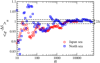
Figure 2: Rogue waves and extreme events of sea-level heights fulfill the integral fluctuation theorem (IFT), which means that statistically the entropy production fluctuates around zero. Here, the computation is applied to the data set from the Japan sea (circles) and the North sea (squares). For the former, since the modeling can be performed for arbitrarily large time windows, it is possible to observe the good convergence towards one ($\Delta\to 0$). In the case of these observational data sets one finds $\Delta\lesssim 1\%$.

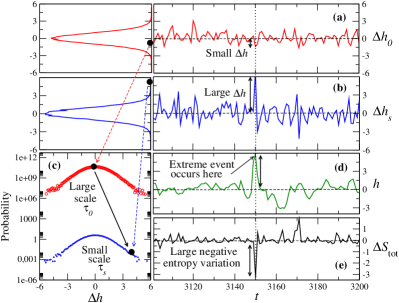
Figure 3: The close relation between an extreme event, i.e. a large fluctuation of a given property, the wave height for rogue waves, within a short time interval, and the entropy production $\Delta S_{{\rm tot}}$: the occurrence of an extreme event is identified by a negative entropy production, $\Delta S_{{\rm tot}}<0$. In (a-b) we illustrate the time series of the height increments $\Delta h_{0,t}=h(t)-h(t-\tau_{0})$ (large scales) and $\Delta h_{s,t}=h(t)-h(t-\tau_{s})$ (small scales) respectively. On the left one sees the corresponding probability distribution for the increments, also plotted (in logarithmic scale) in (c) and shifted vertically for better comparison. (d) The vertical dotted line marks the instant when a rogue wave event takes place: a large value of $h$ emerges. As one sees, (e) the entropy variation is strongly negative, which indicates the statistical feature of a rogue wave or an extreme event in general.

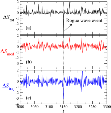
Figure 4: (a) With the total entropy production being negative whenever a rogue wave takes place, one sees that such negative variation of the entropy is not dominated by the variation of the entropy of the medium, $\Delta S_{{\rm med}}$, (b), but rather by the variation of the individual trajectory’s entropy only, $\Delta S_{{\rm traj}}$, (c).

Since the ocean wave system is Markovian in scale, the IFT should also hold for increment ($\Delta h$) trajectories in scale $k$. Based on the knowledge of the Fokker-Planck equation for the system, a total entropy for each increment trajectory can be definedSeifert (2005); Nickelsen and Engel (2013). This total entropy is given by the sum of two contributions,

$$\Delta S_{{\rm tot}}=\Delta S_{{\rm med}}+\Delta S_{{\rm traj}},$$ (4)

with $\Delta S_{{\rm med}}$ being the total entropy variation of the surrounding environment, which, between scales $k$ and $k-1$, is given by

$$(\Delta S_{{\rm med}})_{k,k-1}=-\log{\left(\frac{p(\Delta h_{k-1})}{p(\Delta h_{k})}\right)}.$$ (5)

The contribution $\Delta S_{{\rm traj}}$ is the entropy variation of the system, i.e. along a specific trajectory between those two time scales, and is defined as Seifert (2005)

$$(\Delta S_{{\rm traj}})_{k,k-1}=$$ (6)

$$\int_{\tau_{k}}^{\tau_{k-1}}\frac{\partial}{\partial x}\Delta h(x)\frac{\partial}{\partial\Delta h}\log{\left(p^{{\rm stat}}_{k}(\Delta h,x,h)\right)}dx,$$

where $p^{{\rm stat}}_{k}$ is the stationary solution of Eq. (LABEL:fp)

$$p^{{\rm stat}}_{k}(\Delta h,\tau,h)=\frac{1}{D^{(2)}(\Delta h,\tau,h)}\times\hbox{\large{e}}^{\int_{-\infty}^{\Delta h}\frac{D^{(1)}(x,\tau,h)}{D^{(2)}(x,\tau,h)}dx}.$$ (7)

To obtain $\Delta S_{{\rm tot}}$, the step-wise entropies contributions, defined in Eqs. (5) and (LABEL:enttraj), have to be summed up along the scale trajectories. Figure 1c shows the distribution of $\Delta S_{\rm tot}$ in each one of the data sets.

To show that IFT holds for both data sets we evaluate the Eq. (3) for many events. As shown in Figure 2 the IFT is fulfilled within an accuracy $\lesssim 1\%$ for more than 2000 events. The mean value $\langle e^{-\Delta S}\rangle$ changes very sensitively with variations of the functional form of the Fokker-Planck equation. Thus, the finding of the IFT can also be taken as a strong independent support of the validity of our approach to characterize the complexity of wave states through scale processes. In particular, it supports the thermostatistical description for the emergence of rogue waves here proposed.

The convergence of the average $\langle e^{-\Delta S}\rangle$ is based on a sufficiently large data set, as the exponential function puts much weight on rare negative entropy events. This also means that due to the IFT there must be a special balance between events with positive and negative entropies. This leads us to the next point to set the estimated entropy values for different increment trajectories in connection with wave structures.

Figures 3a and b show time series of the height increments at the largest and smallest scales, $\tau_{0}$ and $\tau_{s}$ respectively, with the corresponding probability distributions (left plots). In Fig. 3c these probability densities are shown in a semi-logarithmic presentation. In Fig. 3d the part of the time series of the corresponding wave height is show. The vertical dotted line marks the rogue wave seen in Fig. 3d, which is characterized by a small height increment at the largest scale and a large increment at the smallest scale. Figure 3c shows that the small increment at the largest scale occurs with a high probability, while the large increment at the smallest scale occurs with low probability.

To each wave height at a particular time instant $t$ belongs a scale trajectory $\Delta h_{k,t}$ in $k$ ($t$ is fixed). Following such scale processes the total entropy variation $\Delta S_{{\rm tot}}$ can be positive (entropy production) or negative (entropy consumption). Comparing the increment time series and the height time series with the series of the corresponding total entropy variations (Fig. 3e) one identifies an abrupt entropy consumption at the time of the occurrence of the rogue wave. As shown in Fig. 4, it is not the entropy of the environment but the entropy of the trajectory which becomes more negative and dominates the occurrence of the extreme event.

Since the negative entropy variation shows to be an indicator of an extreme event, one can now return to Fig. 1c and use the statistical distribution of total entropy variations for predicting how reasonable it is to expect the occurrence of rogue waves at a particular spot in the ocean. The entropy values for the Japan Sea have a distribution shifted to negative values, whereas the measurements taken for the North Sea show a positive mode. Assuming that the Laplacian distribution is a reasonable model for $\Delta S_{\rm tot}$, we can now use the entropy value as a measure for the likelihood of rogue waves. To illustrate this fact, one can see from the distributions $p(\Delta S)$ in Fig. 1c, that an extreme event in the North sea with an amplitude associated to an entropy variation of e.g. $\Delta S_{{\rm tot}}=-6$ is less likely to occur than in the Japan sea by an factor of $10^{-4}$.

In conclusion, we introduce a thermodynamical approach, including the IFT, that enables to interpret the emergence of rogue waves in the context of the statistical physics and provides the possibility for estimate the likelihood of them. An aspect that follows from our framework is that the knowledge of the Fokker-Planck equation for the increment trajectories given by the functions $D^{(1)}(\Delta h,\tau,h)$ and $D^{(2)}(\Delta h,\tau,h)$ can be used also for a simulation of the sea surface elevation Hadjihosseini et al. (2014) (see Supplementary Material I). With such a model it is possible to generate much longer time series to see which further patterns of rogue waves may be expected. Interestingly, preliminary simulations (see Supplementary Material II) indicate that the patterns obtained are qualitatively similar to those obtained from deterministic modeling, like e.g. from solving the non-linear Schrödinger equation, which is today considered a lowest order deterministic model for rogue waves in non-linear media Akhmediev et al. (2011). These results strengthen the indication we provide above that multi-point statistics for sea-level data includes typical features of the alternative deterministic approaches, such as coherent structures. The often debated difference between deterministic models and stochastic approaches seem to fade out for the case investigated here, and can now serve as an inspiration in all fields of science and technology where rare extreme events are known to emerge from a complex dynamical system state, and where at present statistical descriptions fall short of capturing key properties and characterizing the emergence of the extreme events. To name just a few fields where we think the approach presented will be highly influential: in fluid turbulence, where a hierarchy of simultaneous spatial and time scales occurs, our approach might bridge the gap between the statistical approaches to turbulent data and the Navier-Stokes equations; in solid mechanics, ranging from fracture processes, acoustic emissions, up to earthquakes, the approach may be applied, too; and of course also for weather and climate extremes. With our approach the study of rare and extreme events becomes accessible for the wide toolbox of statistical physics, and a completely novel way towards prediction has been opened.

Supplementary material I: Reconstruction of time series with extreme events

Having a stochastic cascade model for the time series of surface heights in the ocean, with or without rogue waves, we are now able to generate data that reproduces all statistical features in the observations, including the ones related to extreme waves.

Figure 5: (a) Rogue waves and extreme events in general fulfill the integral fluctuation theorem (IFT), which means that statistically the entropy production fluctuates around zero. (b) The IFT also holds for the reconstructed data from the stochastic model of Japan Sea heights. Notice that, for the latter, since the modeling can be performed for arbitrarily large time windows, it is possible to observe the good convergence towards one.

Such time series are generated with the $N$-point propagator as mentioned in the article and shown in Hadjihosseini et al. (2016). The starting point is that the process is Markovian in scale, for what evidence is obtained by the verification of $p(\Delta h_{k}|\Delta h_{k+1},\Delta h_{k+2},h)=p(\Delta h_{k}|\Delta h_{k+1},h)$. Assuming that the process is Markovian in scale the $(N+1)$-point propagator

$$p(h_{t}|h_{t-\tau_{1}},...,h_{t-\tau_{N}})=\frac{p(h_{t},h_{t-\tau_{1}},...,h_{t-\tau_{N}})}{p(h_{t-\tau_{1}},...,h_{t-\tau_{N}})}$$ (8)

is used to construct the time series of heights. As the joint multi-point probabilities

$$p(h_{t},h_{t-\tau_{1}},...,h_{t-\tau_{N}})=p(\Delta h_{1},\Delta h_{2},...\Delta h_{N}|h)\cdot p(h)$$ (9)

are equivalent to joint increment statistics, the $(N+1)$-point propagator (of Eq. (8)) can be expressed as

$$p(h_{t}|h_{t-\tau_{1}},...,h_{t-\tau_{N}})=$$ (10)

$$\frac{\prod_{k=1}^{N-1}p(\Delta h_{k}|\Delta h_{k+1},h_{t})}{\prod_{k=2}^{N-1}p(\tilde{\Delta h}_{k},|\tilde{\Delta h}_{k+1},h_{t-\tau_{1}})}\times\frac{p(\Delta h_{N}|h_{t})}{p(\tilde{\Delta h}_{N}|h_{t-\tau_{1}})}\times\frac{p(h_{t})}{p(h_{t-\tau_{1}})}.$$

For reason of clarity we dropped the index $t$ for $\Delta h_{k}$, the two increments $\Delta h_{k}$ and $\tilde{\Delta h}_{k}$ have two different reference points, $h_{t}$ or, respectively $h_{t-\tau_{1}}$. Here we used the Markov property to express all multi-point distributions through simple conditioned probabilities $p(\Delta h_{k}|\Delta h_{k^{\prime}},h)$. Note these conditioned increment probabilities are determined by the Fokker-Planck equation, Eq. (LABEL:fp), for any reference value $h$. The drift and diffusion coefficients are determined from the experimental data, for details see Hadjihosseini et al. (2016). Note that the Fokker-Planck equation is continuous in $\tau$, to obtain results for a finite step size, mentioned above, it has to be iterated over this step.

Figure 5 shows that the IFT is also fulfilled for the numerically reconstructed time series, which we obtain from the estimated Fokker-Planck equations. The same is observed for the North Sea data (not shown). This is again a strong indication that all aspects of our stochastic methods are correct as well as the claim that the correct N-point statistics can be recovered.

Supplementary material II: Statistics and coherent structures in extreme events

As shown in Supplementary Material I, the knowledge of the Fokker-Planck equation for the increment trajectories given by the functions $D^{(1)}(\Delta h,\tau,h)$ and $D^{(2)}(\Delta h,\tau,h)$ can be used for a simulation of the sea surface elevationHadjihosseini et al. (2014). It is possible to generate a time series much longer than the empirical series to see which further patterns of rogue waves may be expected. In sets of such simulated data one can actually observe events that are very similar to real rogue waves. As can be seen in Fig. 6, the rogue wave patterns in our earlier simulations, resemble the ones found in the Japan SeaHadjihosseini et al. (2014).

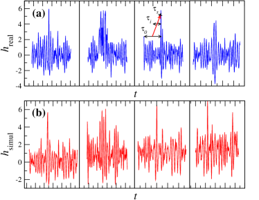
Figure 6: (a) Illustration of pattern in sea-level height series from the Japan Sea during which rogue waves are observed with (b) the corresponding simulations using the stochastic framework based on a Fokker-Planck equation for the distribution of height increments. The similarity between simulated and measured patterns suggests an equivalence between the deterministic and the stochastic description based on what we call a scale-process of the height increments (see text).

Interestingly, these patterns obtained are qualitatively similar to those obtained from deterministic modeling, like e.g. from solving the non-linear Schrödinger equation, which is today considered a lowest order deterministic model for rogue waves in non-linear mediaAkhmediev et al. (2011). These results indicate that the stochastic approach of multi-point statistics presented here also include typical features of the deterministic description, like coherent structures. Thus the often debated difference between deterministic models and stochastic approaches seem to fade out at least for the case investigated here.