A Submodularity-Based Approach for Multi-Agent Optimal Coverage Problems

Abstract

We consider the optimal coverage problem where a multi-agent network is deployed in an environment with obstacles to maximize a joint event detection probability. The objective function of this problem is non-convex and no global optimum is guaranteed by gradient-based algorithms developed to date. We first show that the objective function is monotone submodular, a class of functions for which a simple greedy algorithm is known to be within $1-1/e$ of the optimal solution. We then derive two tighter lower bounds by exploiting the curvature information (total curvature and elemental curvature) of the objective function. We further show that the tightness of these lower bounds is complementary with respect to the sensing capabilities of the agents. The greedy algorithm solution can be subsequently used as an initial point for a gradient-based algorithm to obtain solutions even closer to the global optimum. Simulation results show that this approach leads to significantly better performance relative to previously used algorithms.

I INTRODUCTION

Multi-agent systems involve a team of agents, e.g., vehicles, robots, or sensor nodes, that cooperatively perform one or more tasks in a mission space which may contain uncertainties in the form of obstacles or random event occurrences. Examples of such tasks include environmental monitoring, surveillance, or animal population studies among many. Optimization problems formulated in the context of multi-agent systems, more often than not, involve non-convex objective functions resulting in potential local optima, while global optimality cannot be easily guaranteed.

One of the fundamental problems in multi-agent systems is the optimal coverage problem where agents are deployed so as to cooperatively maximize the coverage of a given mission space [1, 2, 3, 4, 5] where “coverage” is measured in a variety of ways, e.g., through a joint detection probability of random events cooperatively detected by the agents. The problem can be solved by either on-line or off-line methods. Some widely used on-line methods, such as distributed gradient-based algorithms [2, 6, 7] and Voronoi-partition-based algorithms [8, 9, 5], typically result in locally optimal solutions, hence possibly poor performance. To escape such local optima, a “boosting function” approach is proposed in [10] whose performance can be ensured to be no less than that of these local optima. Alternatively, a “ladybug exploration” strategy is applied to an adaptive controller in [11], which aims at balancing coverage and exploration. However, these on-line approaches cannot quantify the gap between the local optima they attain and the global optimum. Off-line algorithms, such as simulated annealing [12, 13], can, under certain conditions, converge to a global optimal solution in probability. However, they are limited by a high computational load and slow convergence rate.

Related to the optimal coverage problem is the “maximum coverage” problem [14, 15], where a collection of discrete sets is given (the sets may have some elements in common and the number of elements is finite) and at most $N$ of these sets are selected so that their union has maximal size (cardinality). The objective function in the maximum coverage problem is submodular, a special class of set functions with attractive properties one can exploit. In particular, a well known result in the submodularity theory [16] is the existence of a lower bound for the global optimum provided by any feasible solution obtained by the greedy algorithm, i.e., an algorithm which iteratively picks the set that covers the maximum number of uncovered elements at each iterative step. Defining, for any integer number $N$ of sets, $L(N)=f/f^{\star}$ where $f^{\star}$ is the global optimum and $f$ is a feasible solution obtained by the greedy algorithm, it is shown in [16] that $L(N)\geq 1-\frac{1}{e}$. In other words, since $f^{\star}\leq(1-\frac{1}{e})^{-1}f$, one can quantify the optimality gap associated with a given solution $f$.

In our past work [10], we studied the optimal coverage problem with agents allowed to be positioned at any feasible point in the mission space (which generally includes several obstacles) and used a distributed gradient-based algorithm to determine optimal agent locations. Depending on initial conditions, a trajectory generated by such gradient-based algorithms may lead to a local optimum. In this paper, we begin by limiting agents to a finite set of feasible positions. An advantage of this formulation is that it assists us in eliminating obviously bad initial conditions for any gradient-based method. An additional advantage comes from the fact that we can show our coverage objective function to be monotone submodular, therefore, a suboptimal solution obtained by the greedy algorithm can achieve a performance ratio $L(N)\geq 1-\frac{1}{e}$, where $N$ is the number of agents in the system. The idea of exploiting the submodularity of the objective function in optimization problems has been used in the literature, e.g., in sensor placement [17, 18] and the maximum coverage problem mentioned above, whereas a total backward curvature of string submodular functions is proposed in [19] and a total curvature $c_{k}$ for the $k$-batch greedy algorithm is proposed in [20] in order to derive bounds for related problems.

Our goal in this paper is to derive a tighter lower bound, i.e., to increase the ratio $L(N)$ by further exploiting the structure of our objective function. In particular, we make use of the total curvature [21] and the elemental curvature [22] of the objective function and show that these can be explicitly derived and lead to new and tighter lower bounds. Moreover, we show that the tightness of the lower bounds obtained through the total curvature and the elemental curvature respectively is complementary with respect to the sensing capabilities of the agents. In other words, when the sensing capabilities are weak, one of the two bounds is tight and when the sensing capabilities are strong, the other bound is tight. Thus, regardless of the sensing properties of our agents, we can always determine a lower bound tighter than $L(N)=1-\frac{1}{e}$ and, in some cases very close to $1$, implying that the greedy algorithm solution can be guaranteed to be near-globally optimal.

Another contribution of the paper is to add a final step to the optimal coverage process, after obtaining the greedy algorithm solution and evaluating the associated lower bound with respect to the global optimum. Specifically, we relax the set of allowable agent positions in the mission space from the imposed discrete set and use the solution of the greedy algorithm as an initial condition for the distributed gradient-based algorithm in [10]. We refer to this as the Greedy-Gradient Algorithm (GGA) which is applicable to the original coverage problem.

The remainder of this paper is organized as follows. The optimal coverage problem is formulated in Sec. II. In Sec. III, we review key elements of the submodularity theory and show that how to apply it to the optimal coverage problem. The GGA for the optimal coverage problem is presented in Sec. IV. In Sec. V, we provide simulation examples to show how the algorithm works and can provide significantly better performance compared to earlier results reported in [10] .

II OPTIMAL COVERAGE PROBLEM FORMULATION

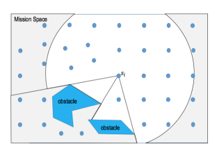
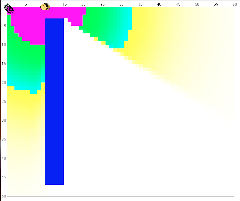
We begin by reviewing the basic coverage problem presented in [4, 8, 6]. A mission space $\Omega\subset\mathbb{R}^{2}$ is modeled as a non-self-intersecting polygon, i.e., a polygon such that any two non-consecutive edges do not intersect. Associated with $\Omega$, we define a function $R(x):\Omega\rightarrow\mathbb{R}$ to characterize the probability of event occurrences at the location $x\in\Omega$. It is referred to as event density satisfying $R(x)\geq 0$ for all $x\in\Omega$ and $\int_{\Omega}R(x)dx<\infty$. The mission space may contain obstacles modeled as $m$ non-self-intersecting polygons denoted by $M_{j}$, $j=1,\ldots,m$, which block the movement as well as the sensing range of an agent. The interior of $M_{j}$ is denoted by $\mathring{M_{j}}$ and the overall feasible space is $F=\Omega\setminus(\mathring{M_{1}}\cup\ldots\cup\mathring{M_{m}})$, i.e., the space $\Omega$ excluding all interior points of the obstacles. There are $N$ agents in the mission space and their positions are defined by a vector $\mathbf{s}=(s_{1},\ldots,s_{N})$ with $s_{i}\in F^{D}$, $i=1,\ldots,N$, where $F^{D}=\{f_{1},\ldots,f_{n}\}$ is a discrete set of feasible positions with cardinality $n$. We assume that $s_{i}\neq s_{j}$ for any two distinct agents $i$ and $j$. Figure 1 shows a mission space with two obstacles and an agent located at $s_{i}$.

In the coverage problem, agents are sensor nodes. We assume that each node has a bounded sensing range captured by the sensing radius $\delta_{i}$. Thus, the sensing region of node $i$ is $\Omega_{i}=\{x:d_{i}(x)\leq\delta_{i}\}$, where $d_{i}(x)=\|x-s_{i}\|$. The presence of obstacles inhibits the sensing ability of a node, which motivates the definition of a visibility set $V(s_{i})\subset F$. A point $x\in F$ is visible from $s_{i}\in F$ if the line segment defined by $x$ and $s_{i}$ is contained in $F$, i.e., $\eta x+(1-\eta)s_{i}\in F$ for all $\eta\in[0,1]$, and $x$ is within the sensing range of $s_{i}$, i.e. $x\in\Omega_{i}$. Then, $V(s_{i})=\Omega_{i}\cap\{x:\eta x+(1-\eta)s_{i}\in F\,\text{for all }\eta\in[0,1]\}$ is a set of points in $F$ which are visible from $s_{i}$. We also define $\bar{V}(s_{i})=F\setminus V(s_{i})$ to be the invisibility set from $s_{i}$, e.g., the grey area in Fig. 1.

Figure 1: Mission space example, $F^{D}$ consists of the blue dots

A sensing model for node $i$ is given by the probability that sensor $i$ detects an event occurrence at $x\in V(s_{i})$, denoted by $p_{i}(x,s_{i})$. We assume that $p_{i}(x,s_{i})$ can be expressed as a function of $d_{i}(x)=\|x-s_{i}\|$ and is monotonically decreasing and differentiable. An example of such a function is

$$p_{i}(x,s_{i})=\exp({-\lambda_{i}\|x-s_{i}\|}),$$ (1)

where $\lambda_{i}$ is a sensing decay factor. For points that are invisible to node $i$, the detection probability is zero. Thus, the overall sensing detection probability, denoted by $\hat{p}_{i}(x,s_{i})$, is defined as

$$\hat{p}_{i}(x,s_{i})=\begin{cases}p_{i}(x,s_{i})&\text{if}\quad x\in V(s_{i}),\\ 0&\text{if}\quad x\in\bar{V}(s_{i}),\end{cases}$$ (2)

which is not a continuous function of $s_{i}$. Note that $V(s_{i})\subset\Omega_{i}=\{x:d_{i}(x)\leq\delta_{i}\}$ is limited by the sensing range of agents $\delta_{i}$ and that the overall sensing detection probability of agents is determined by the sensing range $\delta_{i}$ as well as sensing decay rate $\lambda_{i}$. Then, the joint detection probability that an event at $x\in\Omega$ is detected by the $N$ nodes is given by

$${}P(x,\mathbf{s})=1-\prod_{i=1}^{N}[1-\hat{p}_{i}(x,s_{i})],$$ (3)

where we assume that detection probabilities of different sensors are independent. Assume that $R(x)=0$ for $x\notin F$. The optimal coverage problem can be expressed as follows:

$$\begin{split}\max_{\mathbf{s}}\text{ }&H(\mathbf{s})=\int_{\Omega}R(x)P(x,\mathbf{s})dx\\ \mathrm{s.t.}\quad&\mathbf{s}\in\mathcal{I}\end{split}$$ (4)

where $\mathcal{I}=\{S\subseteq F^{D}:|S|\leq N\}$ is a collection of subsets of $F^{D}$ and $|S|$ denotes the cardinality of set $S$. We emphasize again that $H(\mathbf{s})$ is not convex (concave) even in the simplest possible problem setting.

III SUBMODULARITY THEORY APPLIED TO THE OPTIMAL COVERAGE PROBLEM

A naive method to find the global optimum of (4) is the brute-force search. The time complexity is $n!/(N!(n-N)!)$ by choosing $N$ agent positions from $n$ feasible positions. The brute-force method may not generate quality solutions in a reasonable amount of time when $n$ and $N$ are large. In this section, we will introduce the basic elements of submodularity theory and apply it to the optimal coverage problem. We will show that our objective function $H(\mathbf{s})$ in (4) is monotone submodular, therefore, we can apply basic results from submodularity theory which hold for this class of functions. According to this theory, the greedy algorithm (described in Section I and shown in Algorithm 1) produces a guaranteed performance in polynomial time. The time complexity of the greedy algorithm is $O(nN)$. When $n$ is given, it is $O(N)$, which is linear in the number of agents.

III-A Monotone Submodular Coverage Metric

A submodular function is a set function whose value has the diminishing returns property. The formal definition of submodularity is given as follows.

Definition 1: Given a ground set $Y=\{y_{1},\ldots,y_{n}$} and its power set $2^{Y}$, a function $f:2^{Y}\rightarrow\mathbb{R}$ is called submodular if for any $S,T\subseteq Y$,

$$f(S\cup T)+f(S\cap T)\leq f(S)+f(T).$$ (5)

If, additionally, $f(S)\leq f(T)$ whenever $S\subseteq T$, we say that $f$ is monotone submodular. An equivalent definition, which better reflects the diminishing returns property, is given below, where the proof of equivalence can be found in Appendix A.

Definition 2: For any sets $S,T\subseteq Y$ with $S\subseteq T$ and any $y\in Y\setminus T$, we have

$$f(S\cup\{y\})-f(S)\geq f(T\cup\{y\})-f(T).$$ (6)

Intuitively, the incremental increase of the function is larger when an element is added to a small set than to a larger set. In what follows, we will use the second definition.

A general form of the submodular maximization problem is

$$\begin{split}\max\quad&f(S)\\ \mathrm{s.t.}\quad S&\in\mathcal{I}\end{split}$$ (7)

where $\mathcal{I}$ is a non-empty collection of subsets of a finite set $Y$. $\mathcal{M}=(Y,\mathcal{I}),\mathcal{I}\subseteq 2^{Y}$ is independent if, for all $B\in\mathcal{I}$, any set $A\subseteq B$ is also in $\mathcal{I}$. Furthermore, if for all $A\in\mathcal{I},$ $B\in\mathcal{I}$, $|A|<|B|$, there exists a $j\in B\setminus A$ such that $A\cup\{j\}\in\mathcal{I}$, then $\mathcal{M}$ is called a matroid. Moreover, $\mathcal{M}=(Y,\mathcal{I})$ is called uniform matroid if $\mathcal{I}=\{S\subseteq Y:|S|\leq N\}$.

The following theorem establishes the fact that the objective function $H(\mathbf{s})$ in (4) is monotone submodular, regardless of the obstacles that may be present in the mission space. This will allow us to apply results that quantify a solution obtained through the greedy algorithm relative to the global optimum in (4).

Theorem 1: $H(\mathbf{s})$ is monotone submodular, i.e.,

$$H(S\cup\{s_{k}\})-H(S)\geq H(T\cup\{s_{k}\})-H(T)$$

and

$$H(S)\leq H(T)$$

for any $S,T\subseteq F^{D}$ with $S\subseteq T$ and $s_{k}\in F^{D}\setminus T$.

Proof:

Let $S$ and $T$, such that $S\subseteq T\subseteq F^{D}$, be two agent position vectors. Since $S\subseteq T$ and $0\leq 1-\hat{p}_{i}(x,s_{i})\leq 1$ for any $s_{i}\in F^{D}$, we have

$$\prod_{s_{i}\in S}[1-\hat{p}_{i}(x,s_{i})]\geq\prod_{s_{i}\in T}[1-\hat{p}_{i}(x,s_{i})]$$ (8)

for all $x\in\Omega$. In addition, $H(S\cup\{s_{k}\})$ can be written as

$$\begin{split}&H(S\cup\{s_{k}\})\\ =&\int_{\Omega}R(x)\left\{1-[1-\hat{p}_{k}(x,s_{k})]\prod_{s_{i}\in S}[1-\hat{p}_{i}(x,s_{i})]\right\}dx\\ =&\int_{\Omega}R(x)\left\{1-\prod_{s_{i}\in S}[1-\hat{p}_{i}(x,s_{i})]\right\}dx\\ &+\int_{\Omega}R(x)\hat{p}_{k}(x,s_{k})\prod_{s_{i}\in S}[1-\hat{p}_{i}(x,s_{i})]dx.\end{split}$$

The difference between $H(S)$ and $H(S\cup\{s_{k}\})$ is given by

$$\begin{split}&H(S\cup\{s_{k}\})-H(S)\\ &=\int_{\Omega}R(x)\hat{p}_{k}(x,s_{k})\prod_{s_{i}\in S}[1-\hat{p}_{i}(x,s_{i})]dx.\end{split}$$ (9)

Using the same derivation for $T$, we can obtain

$$\begin{split}&H(T\cup\{s_{k}\})-H(T)\\ &=\int_{\Omega}R(x)\hat{p}_{k}(x,s_{k})\prod_{s_{i}\in T}[1-\hat{p}_{i}(x,s_{i})]dx.\end{split}$$ (10)

From (9) and (10), the difference between $H(S\cup\{s_{k}\})-H(S)$ and $H(T\cup\{s_{k}\})-H(T)$ is

$$\begin{split}&\left[H(S\cup\{s_{k}\})-H(S)\right]-\left[H(T\cup\{s_{k}\})-H(T)\right]\\ =&\int_{\Omega}R(x)\hat{p}_{k}(x,s_{k})\prod_{s_{i}\in S}[1-\hat{p}_{i}(x,s_{i})]dx\\ &-\int_{\Omega}R(x)\hat{p}_{k}(x,s_{k})\prod_{s_{i}\in T}[1-\hat{p}_{i}(x,s_{i})]dx.\end{split}$$ (11)

Using (8), it follows that the difference $[H(S\cup\{s_{k}\})-H(S)]-[H(T\cup\{s_{k}\})-H(T)]\geq 0$. Therefore, from Definition 2, $H(\mathbf{s})$ is submodular.

Next, we prove that $H(\mathbf{s})$ is monotone, i.e., $H(S)\leq H(T)$. Subtracting $H(T)$ from $H(S)$ yields

$$\begin{split}&H(S)-H(T)\\ =&\int_{\Omega}R(x)\left\{1-\prod_{s_{i}\in S}[1-\hat{p}_{i}(x,s_{i})]\right\}dx\\ &-\int_{\Omega}R(x)\left\{1-\prod_{s_{i}\in T}[1-\hat{p}_{i}(x,s_{i})]\right\}dx\\ =&\int_{\Omega}R(x)\left\{\prod_{s_{i}\in T}[1-\hat{p}_{i}(x,s_{i})]-\prod_{s_{i}\in S}[1-\hat{p}_{i}(x,s_{i})]\right\}dx.\end{split}$$

Using (8), we have $H(S)-H(T)\leq 0$. Therefore, $H(\mathbf{s})$ is a monotone submodular function. $\blacksquare$

III-B Greedy Algorithm and Lower Bounds

Finding the optimal solution to (7) is in general NP-hard. The following greedy algorithm is usually used to obtain a feasible solution for (7). The basic idea of the greedy algorithm is to add an agent which can maximize the value of the objective function at each iteration.

Algorithm 1 Greedy Algorithm

0:  Submodular function $f(S)$Cardinality constraint $N$

0:  Set $S$Initialization: $S\leftarrow\emptyset$, $i\leftarrow 0$

1:  while $i\leq N$ do

2:     $s_{i}^{\ast}=\operatorname*{\arg\!\max}_{s_{i}\in Y\setminus S}{f(S\cup\{s_{i}\})}$

3:     $S\leftarrow S\cup\{s_{i}^{\ast}\}$

4:     $i\leftarrow i+1$

5:  end while

6:  return  $S$

In the following analysis, we assume that $f$ is a monotone submodular function satisfying $f(\emptyset)=0$ and $\mathcal{M}=(Y,\mathcal{I})$ is a uniform matroid. We will use the definition

$$L(N)=\frac{f}{f^{\ast}}$$

from Section I, where $f^{\star}$ is the global optimum of (7) and $f$ is a feasible solution obtained by Algorithm 1. Then, as shown in [16], a lower bound of $L(N)$ is $1-1/e$ .

Next, we consider the total curvature

$$c=\max_{j\in Y}\left[1-\frac{f(Y)-f(Y\setminus j)}{f(\{j\})}\right]$$ (12)

introduced in [21]. Using $c$, the lower bound of $L(N)$ above is improved to be $T(c,N)$:

$$T(c,N)=\frac{1}{c}\left[1-(\frac{N-c}{N})^{N}\right].$$ (13)

where $c\in[0,1]$, and

$$T(c,N)\geq 1-\frac{1}{e}$$

for any $N\geq 1$. If $c=1$, the result is the same as the bound obtained in [16], [23].

In addition, we consider the elemental curvature

$$\alpha=\max_{S\subset Y,i,j\in Y\setminus S,i\neq j}\frac{f(S\cup\{i,j\})-f(S\cup\{j\})}{f(S\cup\{i\})-f(S)},$$ (14)

based on which the following bound is obtained:

$$E(\alpha,N)=1-\left(\frac{\alpha+\ldots+\alpha^{N-1}}{1+\alpha+\ldots+\alpha^{N-1}}\right)^{N}$$ (15)

and it is shown in [22] that $L(N)\geq E(\alpha,N)$. Note that $E(\alpha,N)$ can be simplified as follows:

$$E(\alpha,N)=\begin{cases}1-(\frac{N-1}{N})^{N},&\text{when }\alpha=1;\\ 1-(\frac{\alpha-\alpha^{N}}{1-\alpha^{N}})^{N},&\text{when }0\leq\alpha<1.\end{cases}$$ (16)

If both bounds $T(c,N)$ and $E(\alpha,N)$ can be calculated, then the larger one will be the lower bound $L(N)$, defined as

$$L(N)=\max\{T(c,N),E(\alpha,N)\}.$$ (17)

Accordingly, we have $f(S)\geq L(N)f(S^{\ast})$, where $S^{\star}$ is the global optimum set, and $S$ is the set obtained by Algorithm 1.

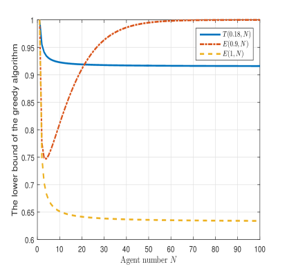
Figure 2 shows the dependence of $T(c,N)$ and $E(\alpha,N)$ on the number of agents $N$ for some specific values of $c$ and $\alpha$ (as shown in the figure). Clearly, if $c<1$ and $\alpha<1$, then $L(N)$ in (17) is much tighter than $1-\frac{1}{e}$.

Figure 2: $T(c,N)$ and $E(\alpha,N)$ as a function of the number of agents $N$

III-C Curvature Information Calculation

In this subsection, we will derive the concrete form of the total curvature $c$ and the elemental curvature $\alpha$ in the context of coverage problems. For notational convenience, $\hat{p}_{i}(x,s_{i})$ is used without its arguments as long as this dependence is clear from the context.

Recall that $F^{D}$ is the set of feasible agent positions. We can obtain from (4):

$${}\begin{split}H(F^{D})&=\int_{\Omega}R(x)\left[1-\prod_{i=1}^{n}(1-\hat{p}_{i})\right]dx\\ &=\int_{\Omega}R(x)\left[1-(1-\hat{p}_{j})\prod_{i=1,i\neq j}^{n}(1-\hat{p}_{i})\right]dx,\end{split}$$

and

$${}H(F^{D}\setminus\{s_{j}\})=\int_{\Omega}R(x)\left[1-\prod_{i=1,i\neq j}^{n}(1-\hat{p}_{i})\right]dx.$$

The difference between $H(F^{D})$ and $H(F^{D}\setminus\{s_{j}\})$ is

$$H(F^{D})-H(F^{D}\setminus\{s_{j}\})=\int_{\Omega}R(x)\hat{p}_{j}\prod_{i=1,i\neq j}^{n}[1-\hat{p}_{i}]dx.$$ (18)

When there is only one agent $s_{j}$, the objective function is

$$H(s_{j})=\int_{\Omega}R(x)\hat{p}_{j}dx.$$ (19)

Combining (12), (18) and (19), we obtain

$$c=\max_{s_{j}\in F^{D}}\left[1-\frac{\int_{\Omega}R(x)\hat{p}_{j}\prod_{i=1,i\neq j}^{n}[1-\hat{p}_{i}]dx}{\int_{\Omega}R(x)\hat{p}_{j}dx}\right].$$ (20)

Remark 1 If the sensing capabilities of agents are weak, that is, $\hat{p}_{i}$ is small for most parts in the mission space, then $\prod_{i=1,i\neq j}^{n}(1-\hat{p}_{i})$ is, in turn, close to 1, which leads to a small value of $c$. It follows from (13) that the lower bound $T(c,N)$ is a monotonically decreasing function of $c$ and approaches 1 near $c=0$. This implies that the solution of the greedy algorithm is very close to the global optimum when the sensing capabilities are weak.

Next, we calculate the elemental curvature $\alpha$. From (9), the difference between $H(S)$ and $H(S\cup\{s_{k}\})$ is

$$H(S\cup\{s_{k}\})-H(S)=\int_{\Omega}R(x)\hat{p}_{k}(x)\prod_{s_{i}\in S}[1-\hat{p}_{i}]dx.$$ (21)

Using the same derivation, we can obtain

$$\begin{split}&H(S\cup\{s_{j},s_{k}\})-H(S\cup\{s_{j}\})\\ &\qquad=\int_{\Omega}R(x)\hat{p}_{k}(1-\hat{p}_{j})\prod_{s_{i}\in S}[1-\hat{p}_{i}]dx.\end{split}$$ (22)

The elemental curvature in (14) can then be calculated by

$$\begin{split}\alpha&=\max_{S,s_{j},s_{k}}\frac{H(S\cup\{s_{j},s_{k}\})-H(S\cup\{s_{j}\})}{H(S\cup\{s_{k}\})-H(S)}\\ &=\max_{S,s_{j},s_{k}}\frac{\int_{\Omega}R(x)\hat{p}_{k}(1-\hat{p}_{j})\prod_{s_{i}\in S}[1-\hat{p}_{i}]dx}{\int_{\Omega}R(x)\hat{p}_{k}\prod_{s_{i}\in S}[1-\hat{p}_{i}]dx}\\ &=\max_{S,s_{j},s_{k}}1-\frac{\int_{\Omega}R(x)\hat{p}_{k}\hat{p}_{j}\prod_{s_{i}\in S}[1-\hat{p}_{i}]dx}{\int_{\Omega}R(x)\hat{p}_{k}\prod_{s_{i}\in S}[1-\hat{p}_{i}]dx}\\ &=1-\min_{s_{j},x\in\Omega}\hat{p}_{j}(x,s_{j}).\end{split}$$ (23)

Remark 2 Observe that the elemental curvature turns out to be determined by a single agent. If there exists a pair $(x,s_{j})$ such that $x\in\bar{V}(s_{j})$ in (2), then $\hat{p}_{j}(x,s_{j})=0$ and $\alpha=1$. This may happen when there are obstacles in the mission space or the sensing capabilities of agents are weak (e.g., the sensing range is small or the sensing decay rate is large). On the other hand, if the sensing capabilities are so strong that $\hat{p}_{j}(x,s_{j})\neq 0$ for any $x\in F,s_{j}\in F^{D}$, then $\alpha<1$. In addition, $E(\alpha,N)$ is a monotonically decreasing function of $\alpha$.

An interesting conclusion from this analysis is that $T(c,N)$ and $E(\alpha,N)$ are complementary with respect to the sensing capabilities of sensors. From Remark 1, $T(c,N)$ is large when the sensing capabilities are weak, while from Remark 2, $E(\alpha,N)$ is large when the sensing capabilities are strong. This conclusion is graphically depicted in Figs. 3 and 4 (where sensing capability varies from strong to weak). In Fig. 3, $E(\alpha,N)$ and $T(c,N)$ have been evaluated for $N=10$ and $\delta=80$ as a function of one of the measures of sensing capability, the sensing decay rate $\lambda$ in (1), assuming all agents have the same sensing capabilities. One can see that for small values of $\lambda$, the bound $E(\alpha,10)$ is close to 1 and dominates both $T(c,10)$ and the well-known bound $1-\frac{1}{e}$. Beyond a critical value of $\lambda$, it is $T(c,10)$ that dominates and approaches 1 for large values of $\lambda$. Figure 4 shows a similar behavior when $T(c,N)$ and $E(\alpha,N)$ are evaluated for $N=10$ and $\lambda=0.03$ as a function of the other measure of sensing capability, the sensing range $\delta$. When the sensing range exceeds the distance of the diagonal of the mission space, there is no value in further increasing the sensing range and $E(\cdot)$ becomes constant. When $\delta>20$, the sensing capabilities are strong and $T(\cdot)$ becomes constant. Therefore, both $E(\cdot)$ and $T(\cdot)$ become constant when $\delta$ exceeds corresponding thresholds. On the other hand, when the sensing range is smaller than some threshold, then $\alpha=1$, and $E(1,10)=0.6513$.

Figure 3: Lower bound $L(10)$ as a function of the sensing decay rate of agents

Figure 4: Lower bound $L(10)$ as a function of the sensing range of agents

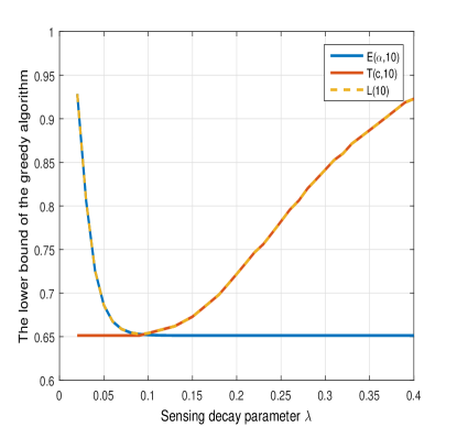
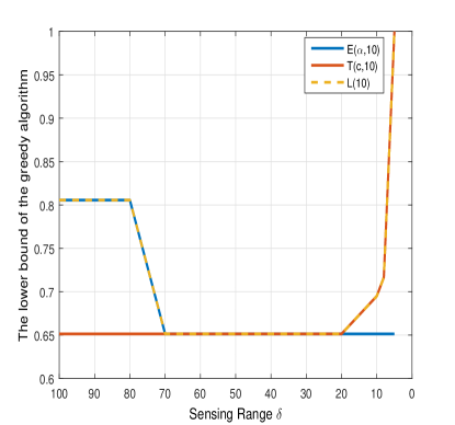
Figures 3 and 4 also illustrate the trade-off between the sensing capabilities and the coverage performance guarantee. Agents with strong capabilities obviously achieve better coverage performance. On the other hand, one can get a better guaranteed performance as the agents’ capabilities get weaker. Therefore, if one is limited to agents with weak sensing capabilities in a particular setting, the use of $T(c,N)$ is appropriate and this trade-off may be exploited.

IV GREEDY-GRADIENT ALGORITHM

Thus far, we have restricted agent positions to be selected from the finite feasible set $f^{D}=\{f_{1},...,f_{n}\}$. In this section, agents are allowed to be deployed at any feasible point, and the optimal coverage problem becomes

$$\begin{split}\max_{\mathbf{s}}\text{ }&H(\mathbf{s})=\int_{\Omega}R(x)P(x,\mathbf{s})dx\\ \mathrm{s.t.}\quad&s_{i}\in F,i=1,...,N.\end{split}$$ (24)

We propose a Greedy-Gradient Algorithm (GGA) shown in Algorithm 2 to solve this problem. The basic idea is to use existing gradient-based algorithms with an initial deployment given by the greedy algorithm (Algorithm 1) to seek better performance. In particular, we use the distributed gradient-based algorithm developed in [6]:

$$s_{i}^{k+1}=s_{i}^{k}+\zeta_{k}\frac{\partial H(\mathbf{s})}{\partial s_{i}^{k}},\text{ \ }k=0,1,\ldots$$ (25)

where the step size sequence $\{{\zeta_{k}\}}$ is appropriately selected to ensure convergence of the resulting trajectories for all agents [24]. The detailed calculation of $\frac{\partial H(\mathbf{s})}{\partial s_{i}^{k}}$ can be found in [10].

Algorithm 2 Greedy-Gradient Algorithm

0:  Objective function $H(\textbf{s})$

0:  Agent positions sInitialization: s given by Greedy Algorithm 1

1:  while the stopping criterion is not satisfied do

2:     Choose a step size $\zeta>0$

3:     for $i=1,\ldots,N$ do

4:        Determine a searching direction $\frac{\partial H(\mathbf{s})}{\partial s_{i}}$

5:        Update: $s_{i}\leftarrow s_{i}+\zeta\frac{\partial H(\mathbf{s})}{\partial s_{i}}$

6:     end for

7:  end while

8:  return  s

The stopping criterion is of the form $\|\frac{\partial H(\mathbf{s})}{\partial s_{i}}\|\leq\eta$, where $\eta$ is a small positive scalar.

V SIMULATION RESULTS

In this section, we illustrate through simulation our analysis and the use of the GGA (Algorithm 2) for coverage problems in a variety of mission spaces with and without obstacles. The mission space is a $60\times 50$ rectangular area and the event density function $R(x)$ is assumed to be uniformly distributed, i.e., we set $R(x)=1$ in (4). We first compute the theoretical lower bound $L(N)$ for the case of no obstacles in the mission space and the number of agents is $N=10$.

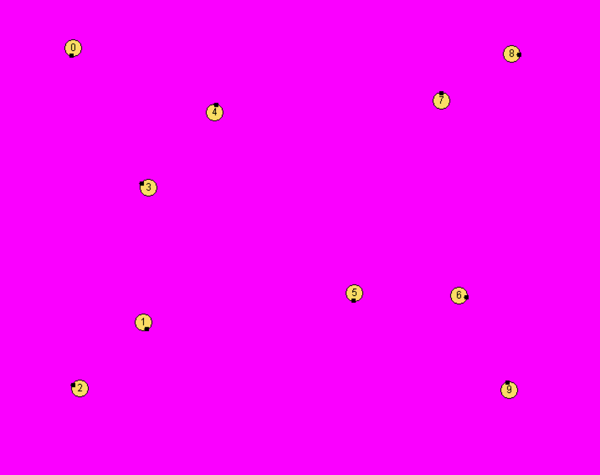
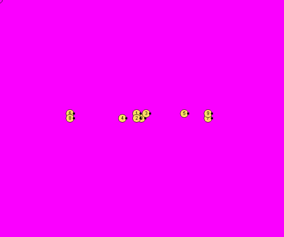
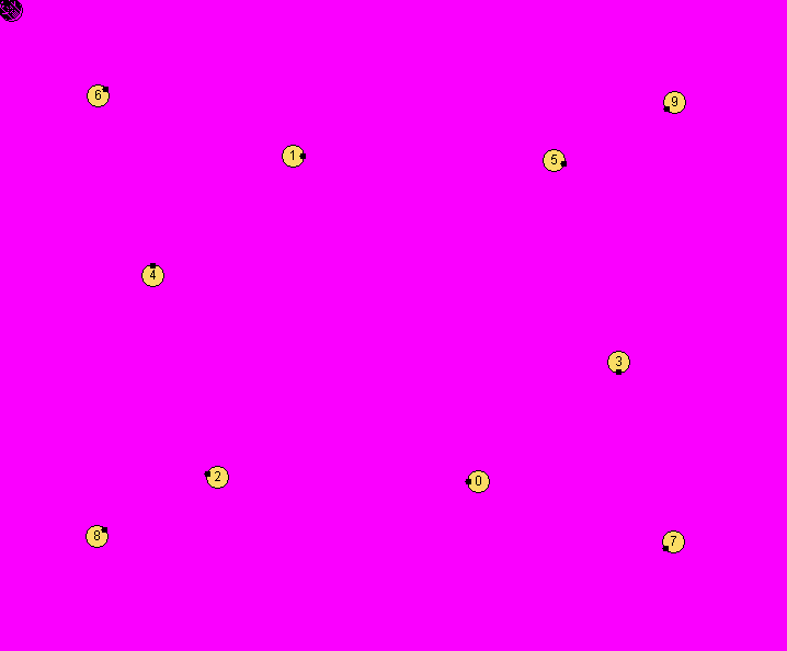
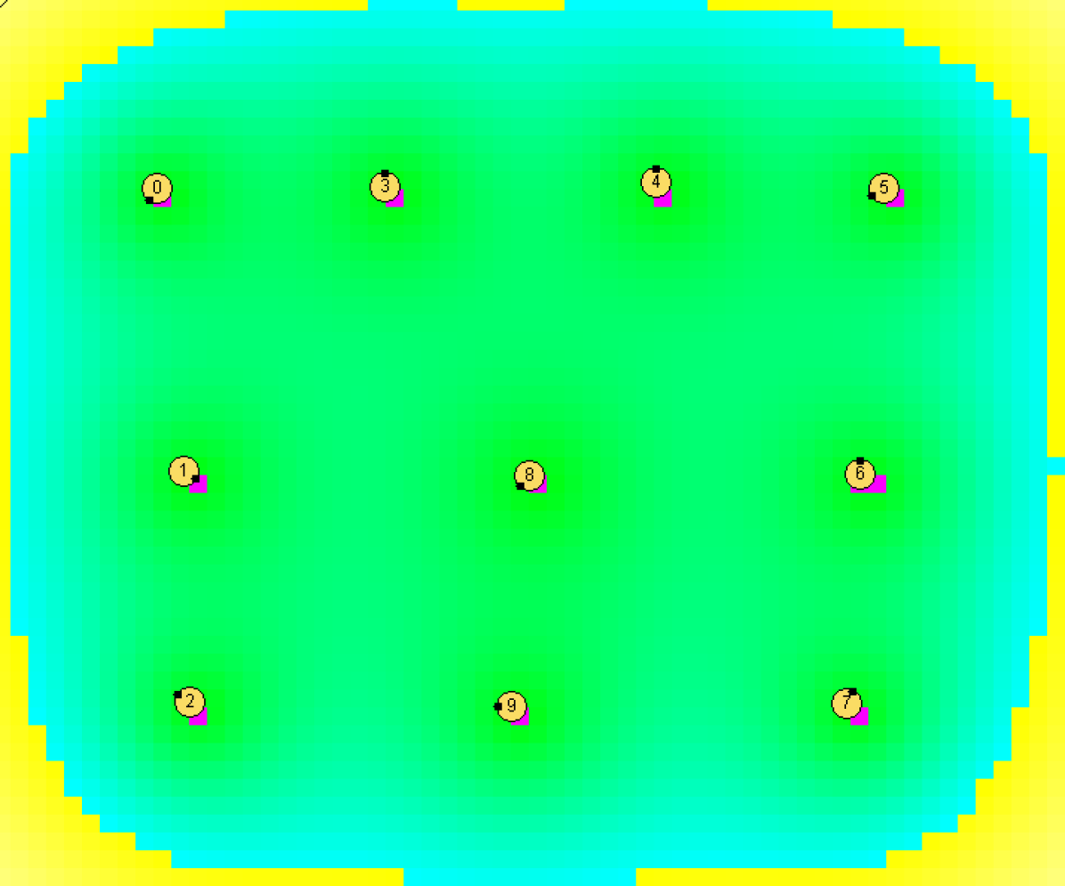
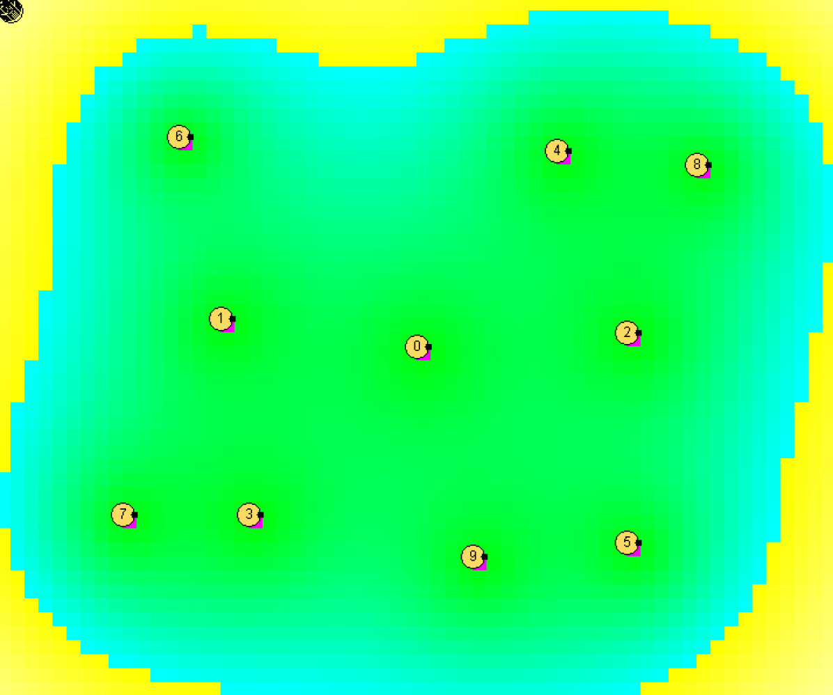
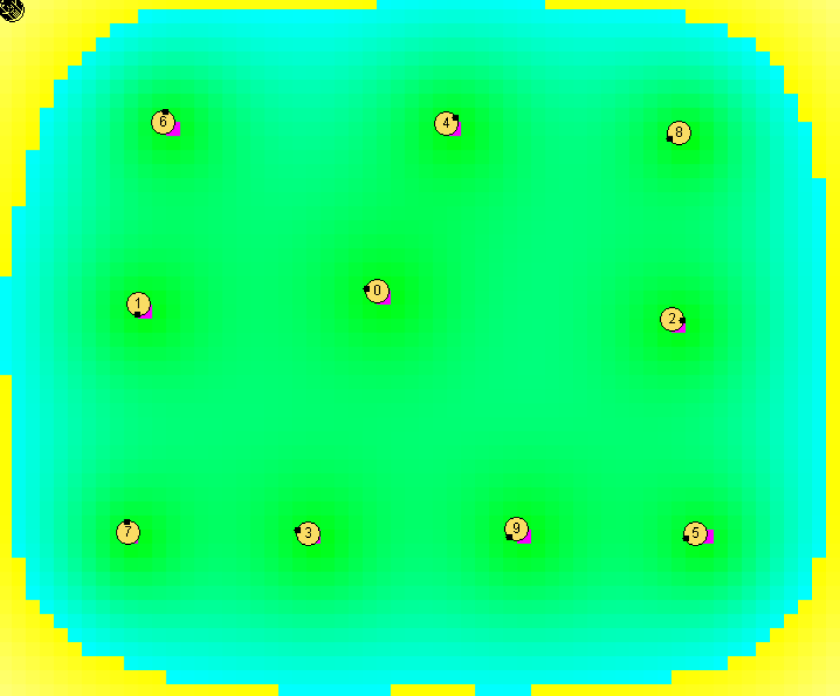
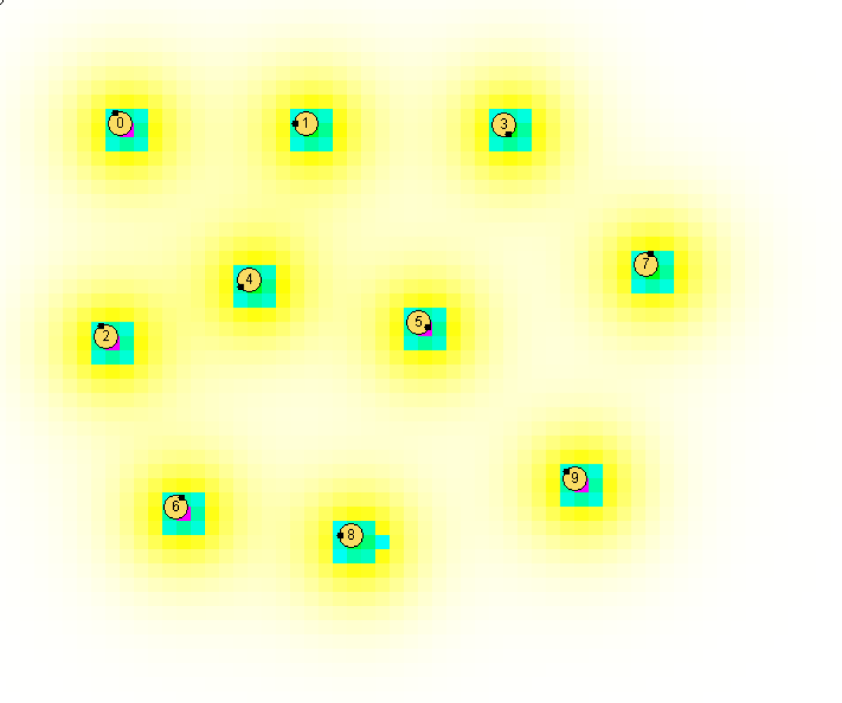
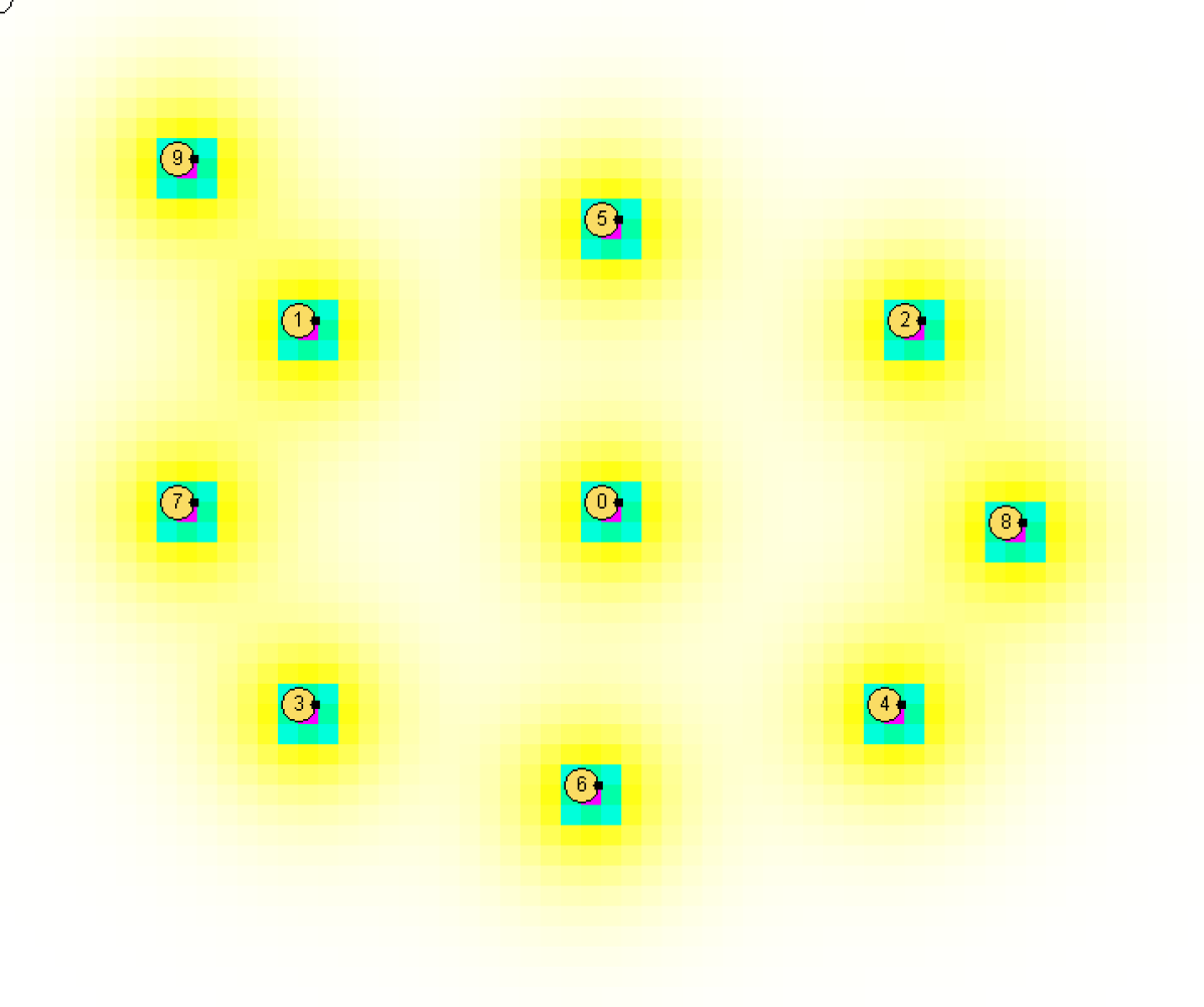
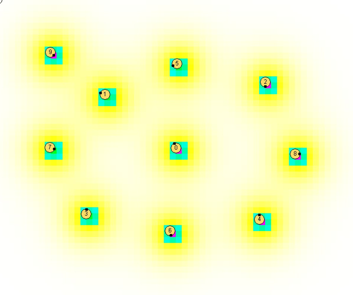
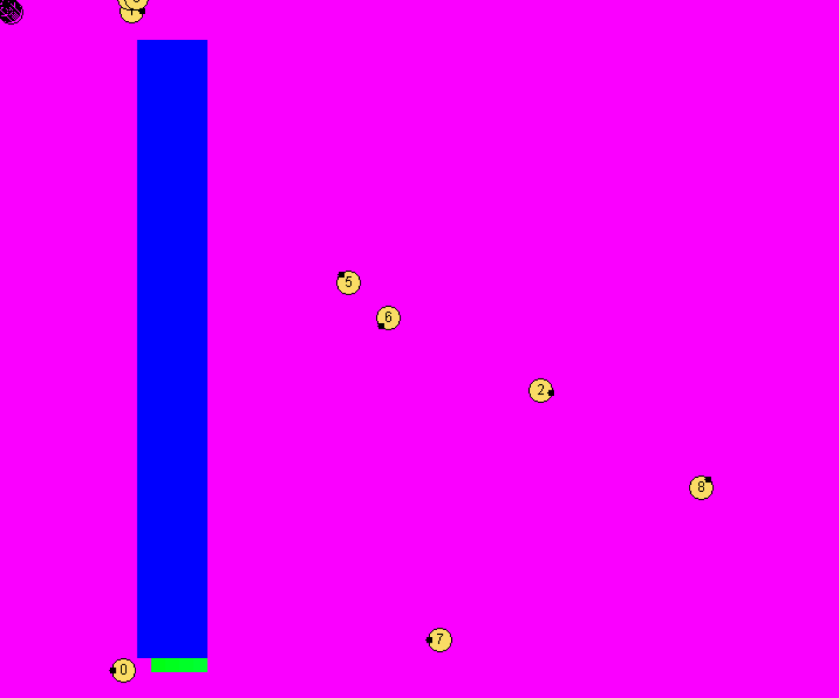
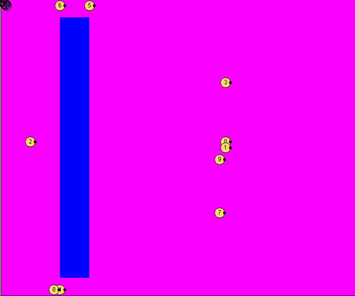
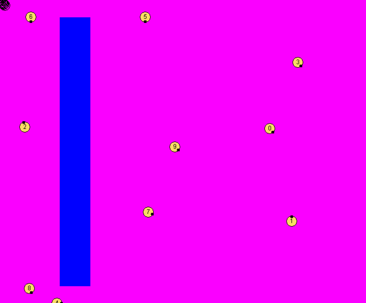
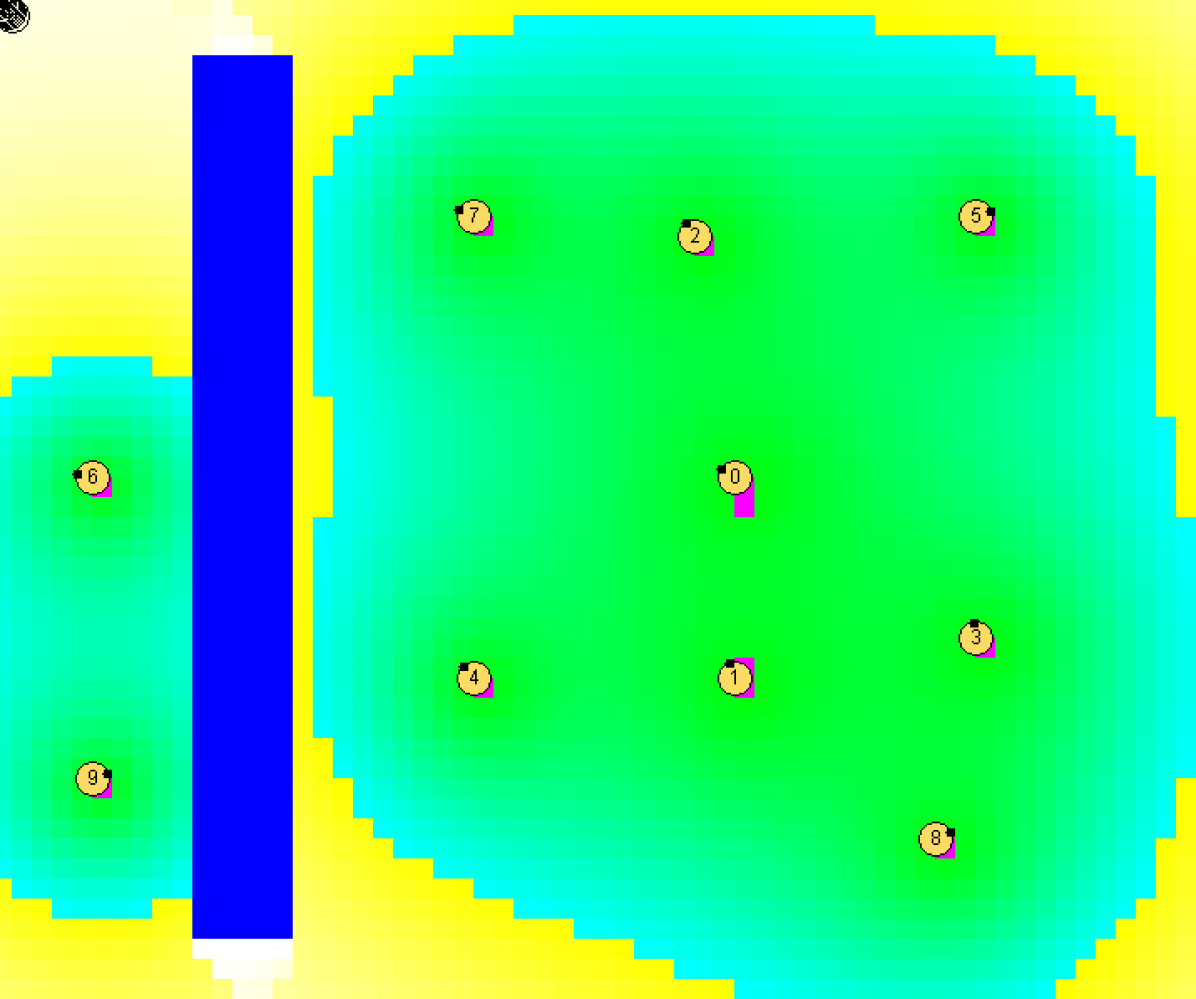
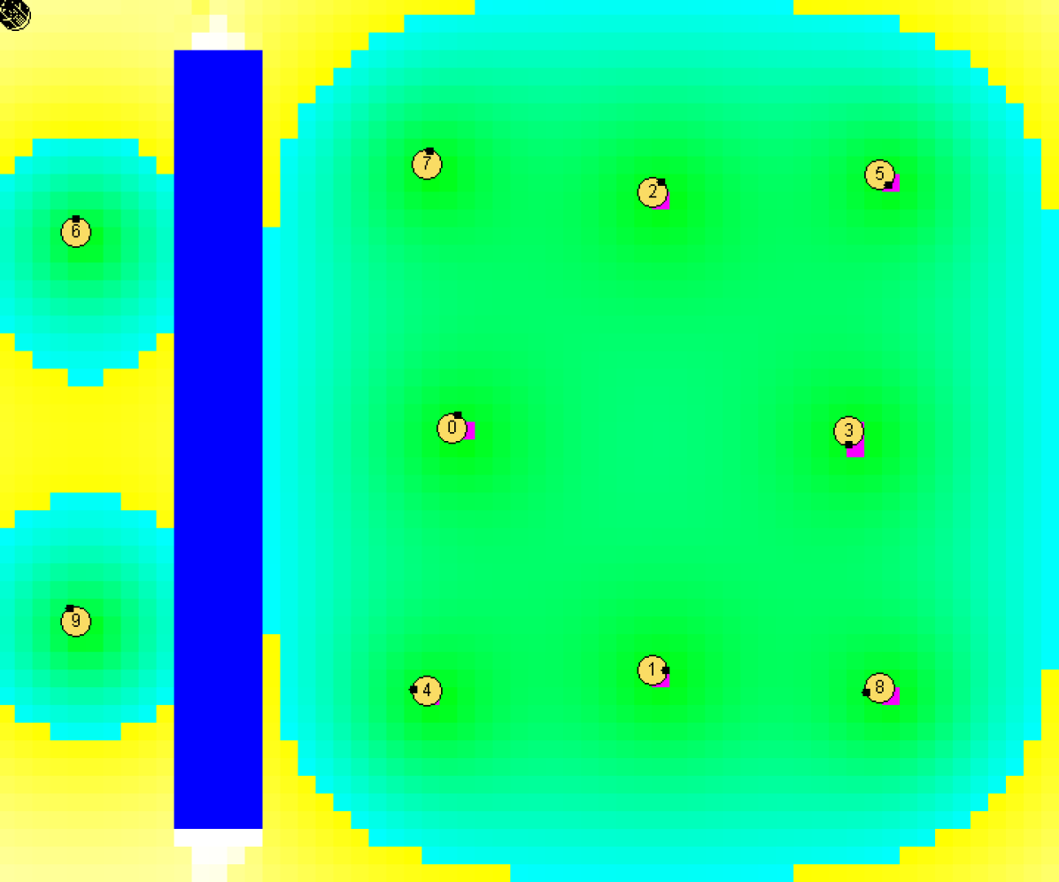
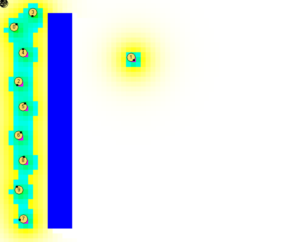
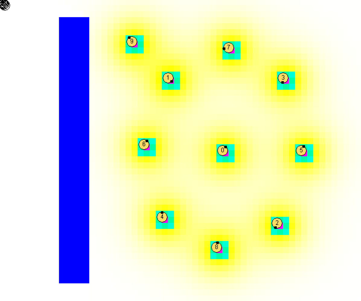
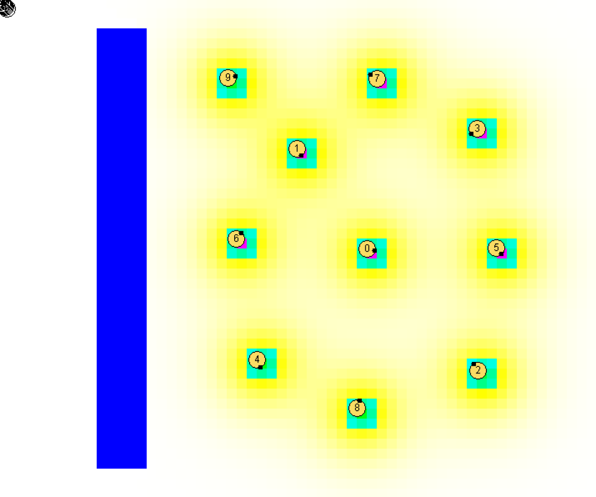
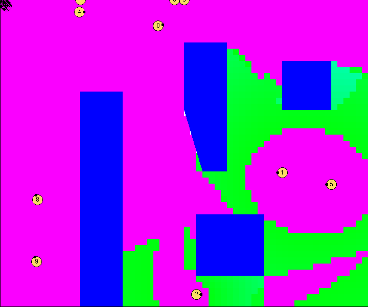
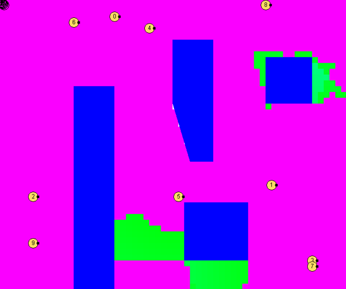
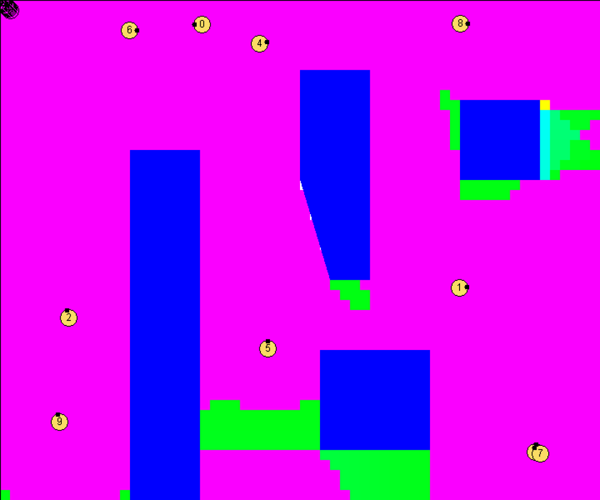
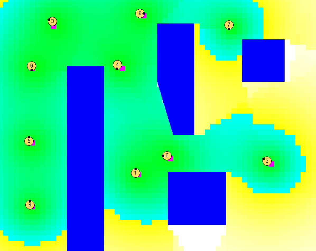
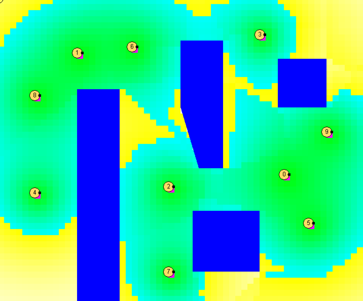
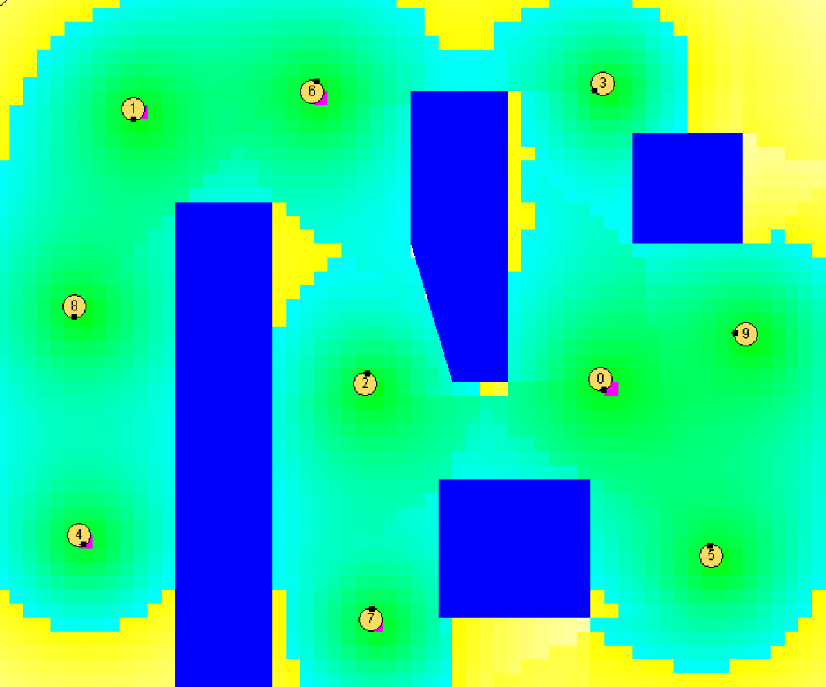
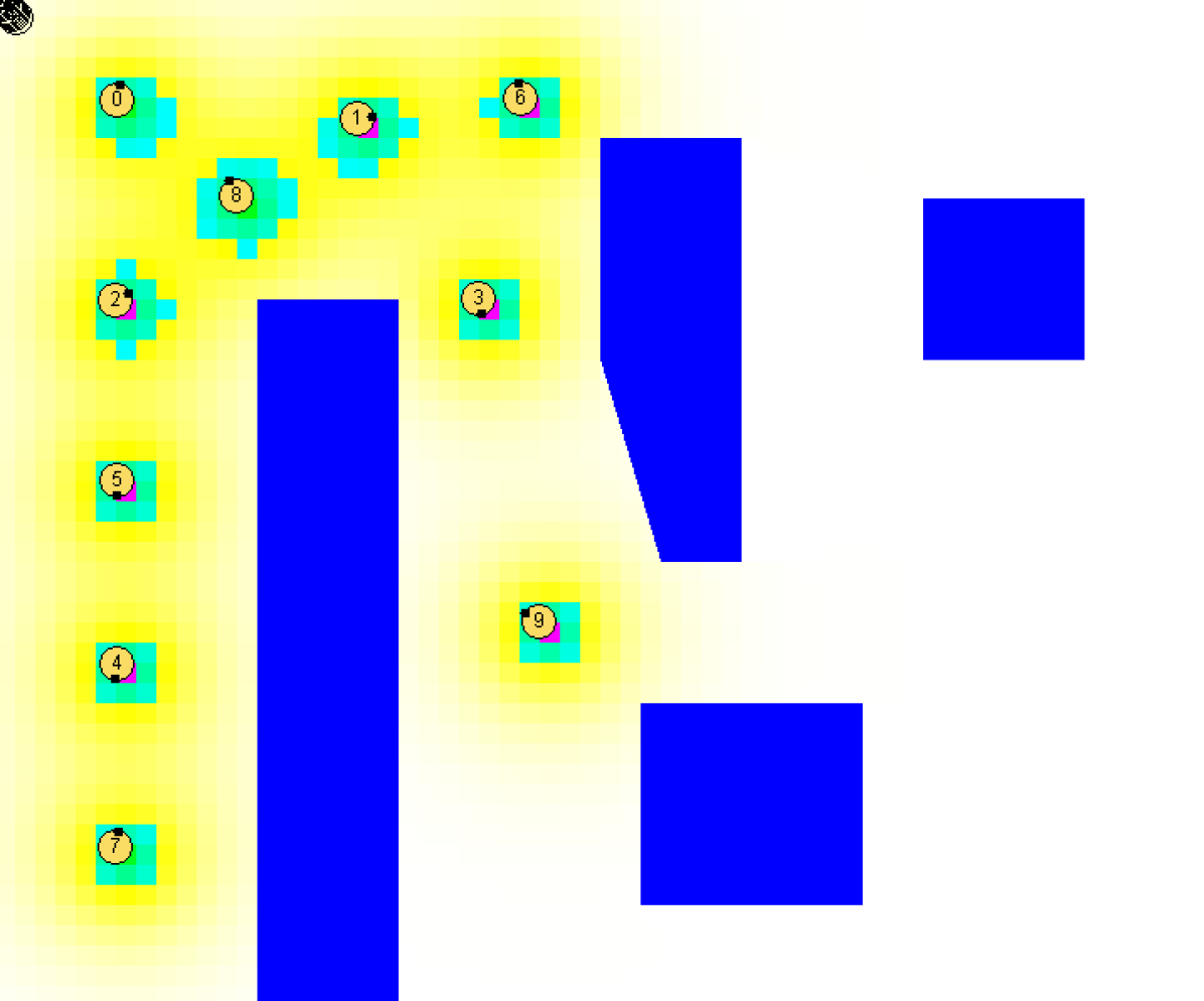
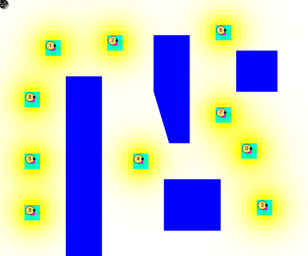
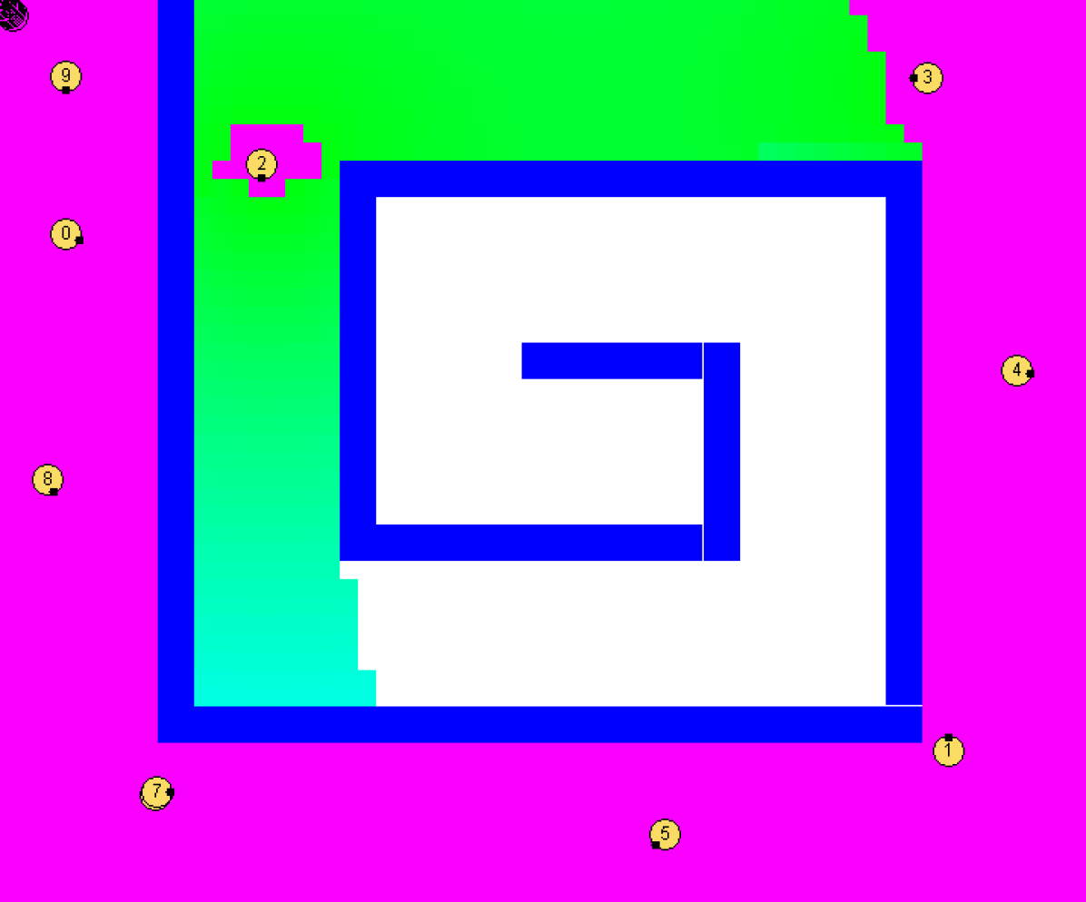
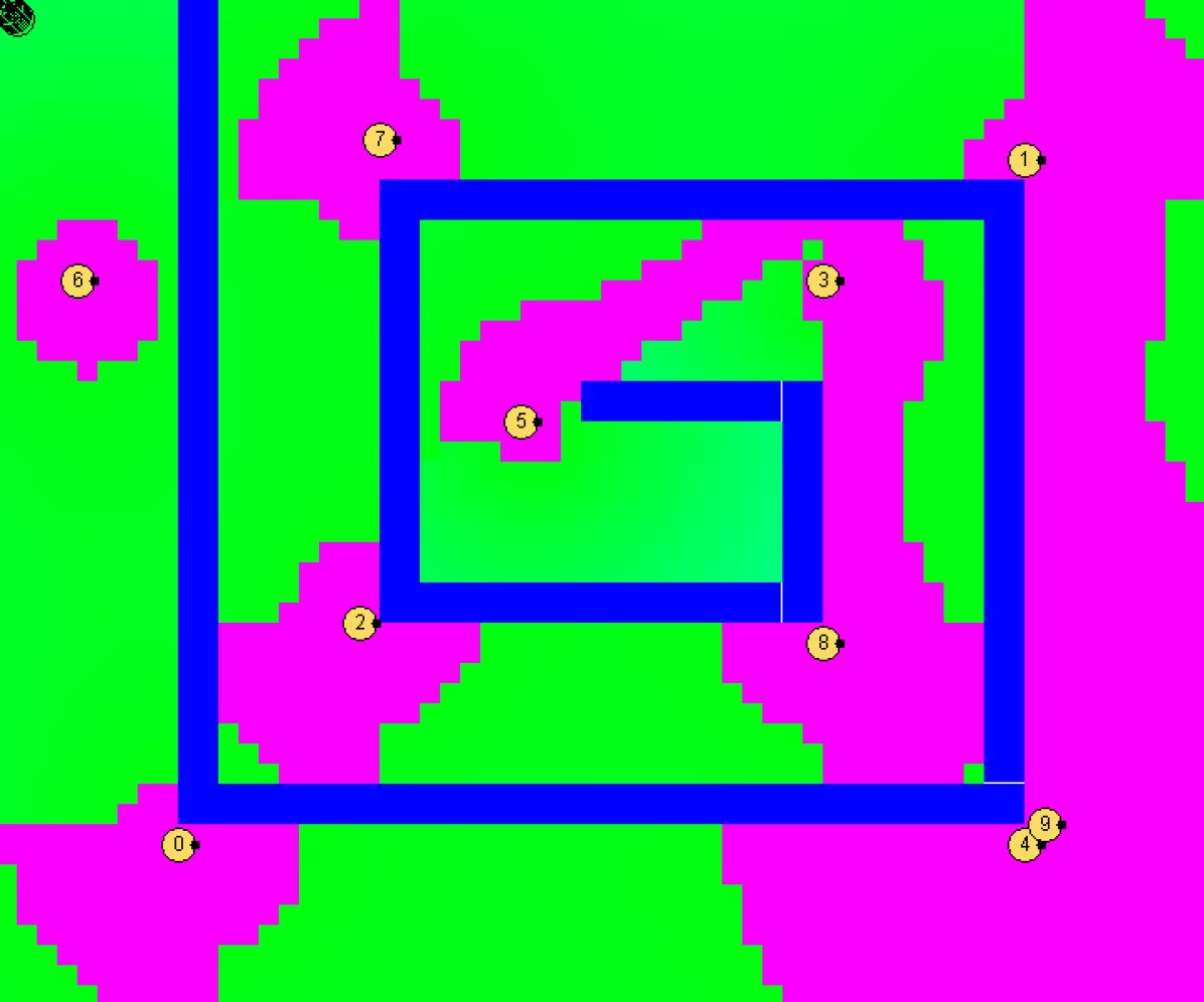
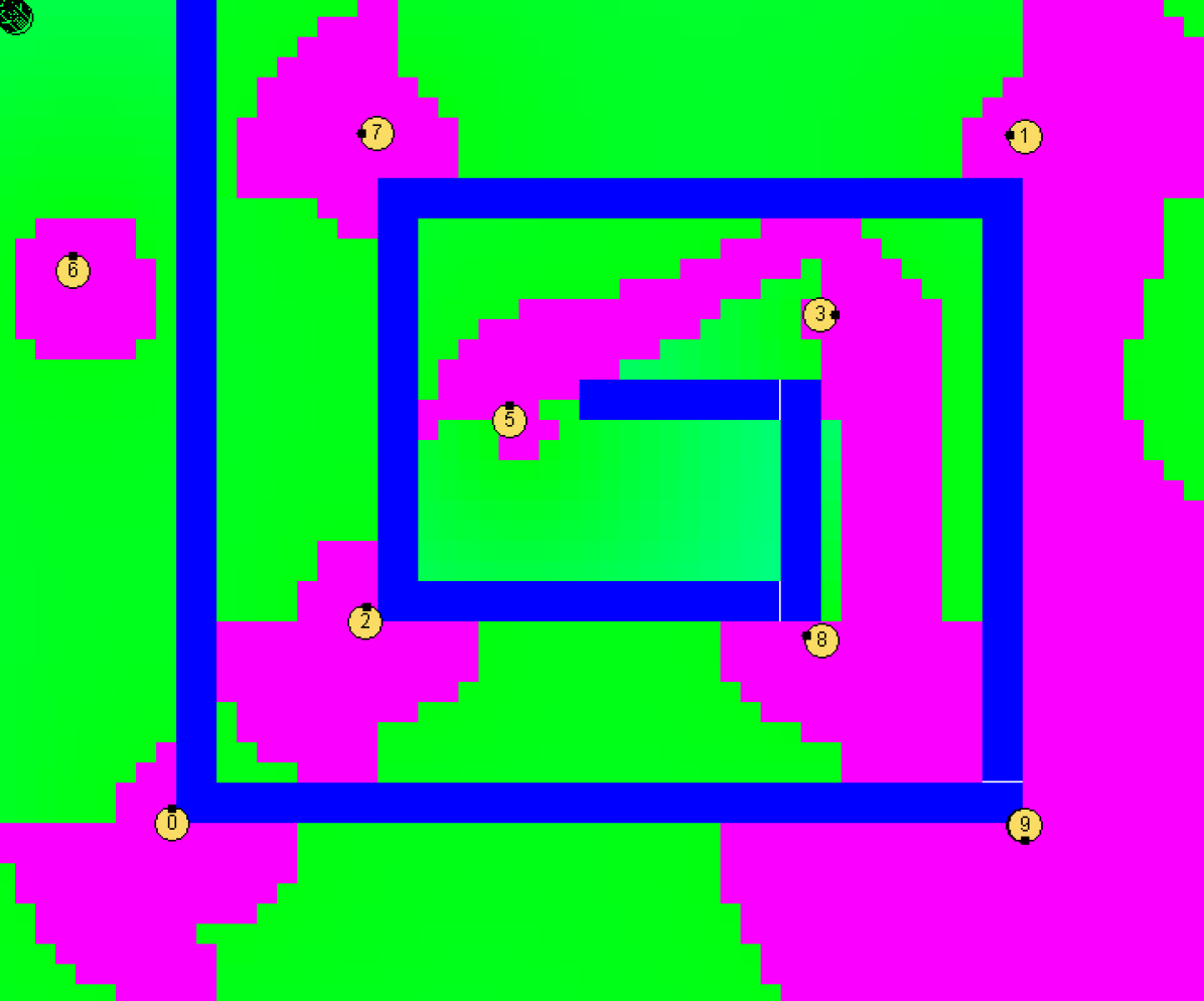
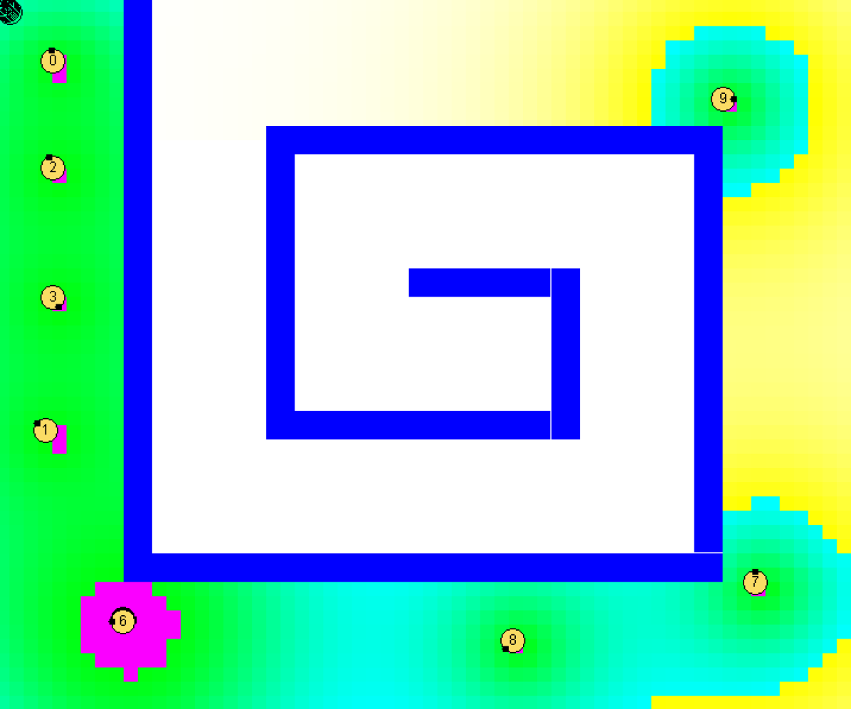
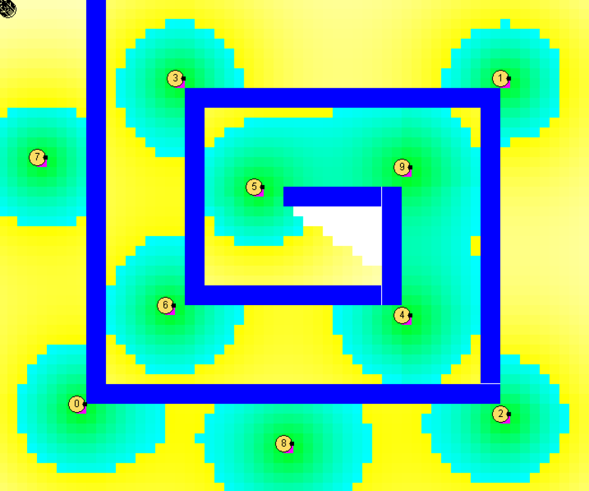
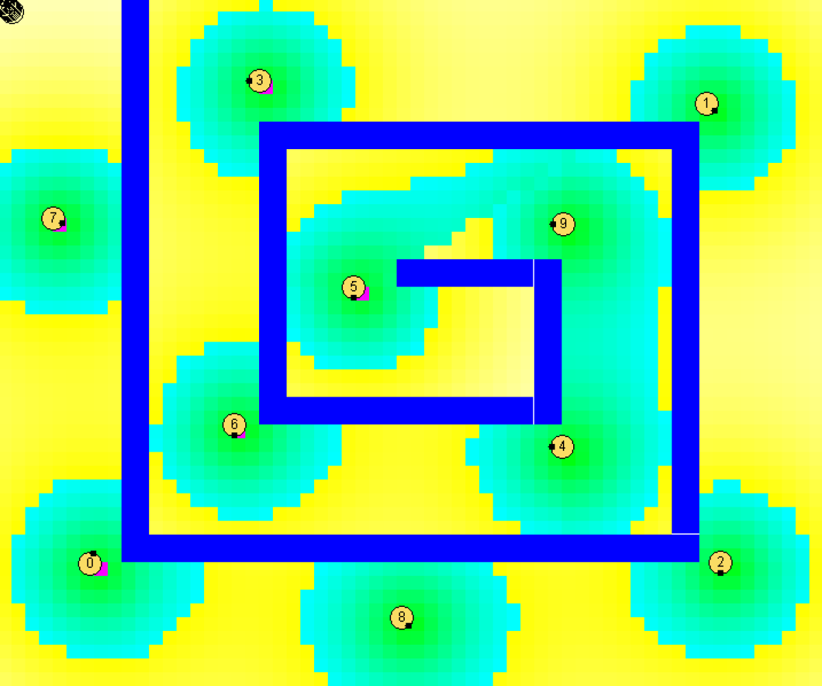
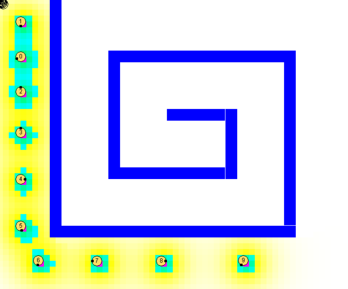
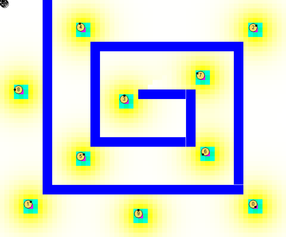
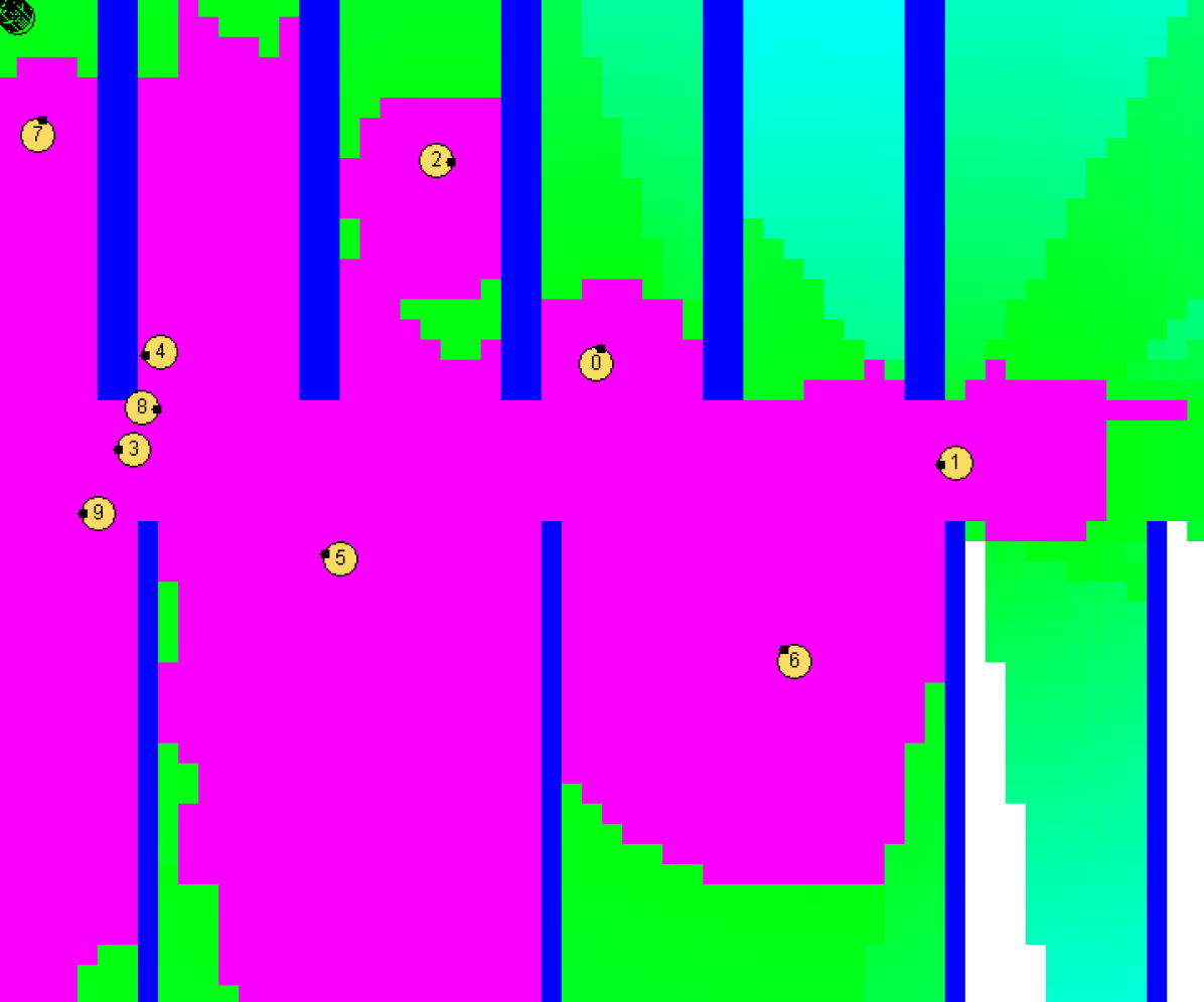
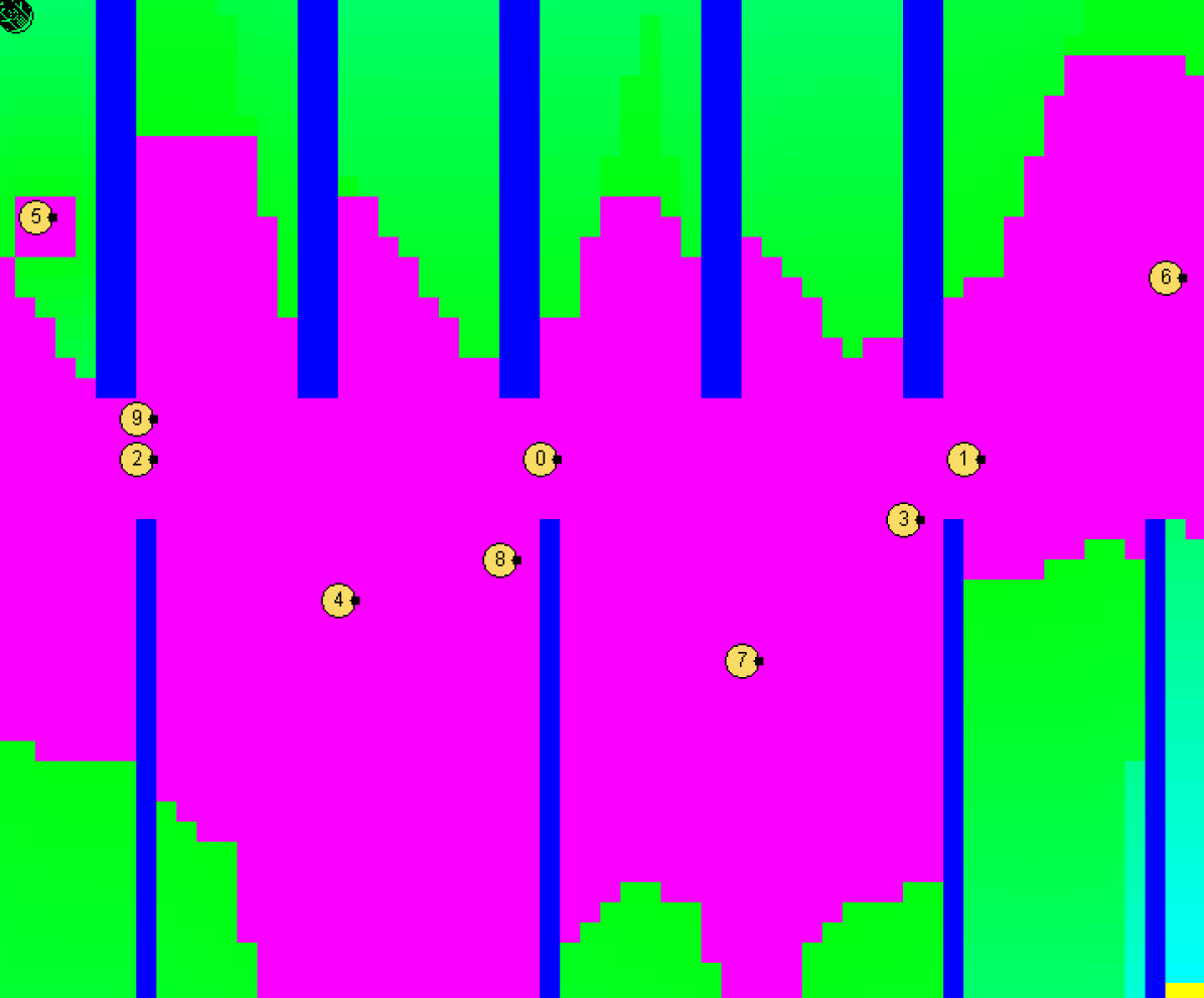
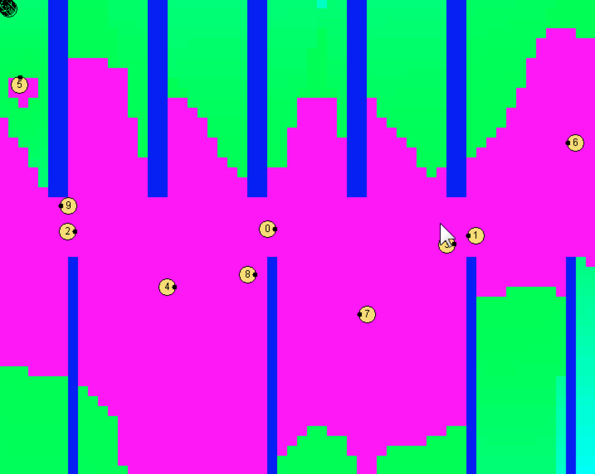
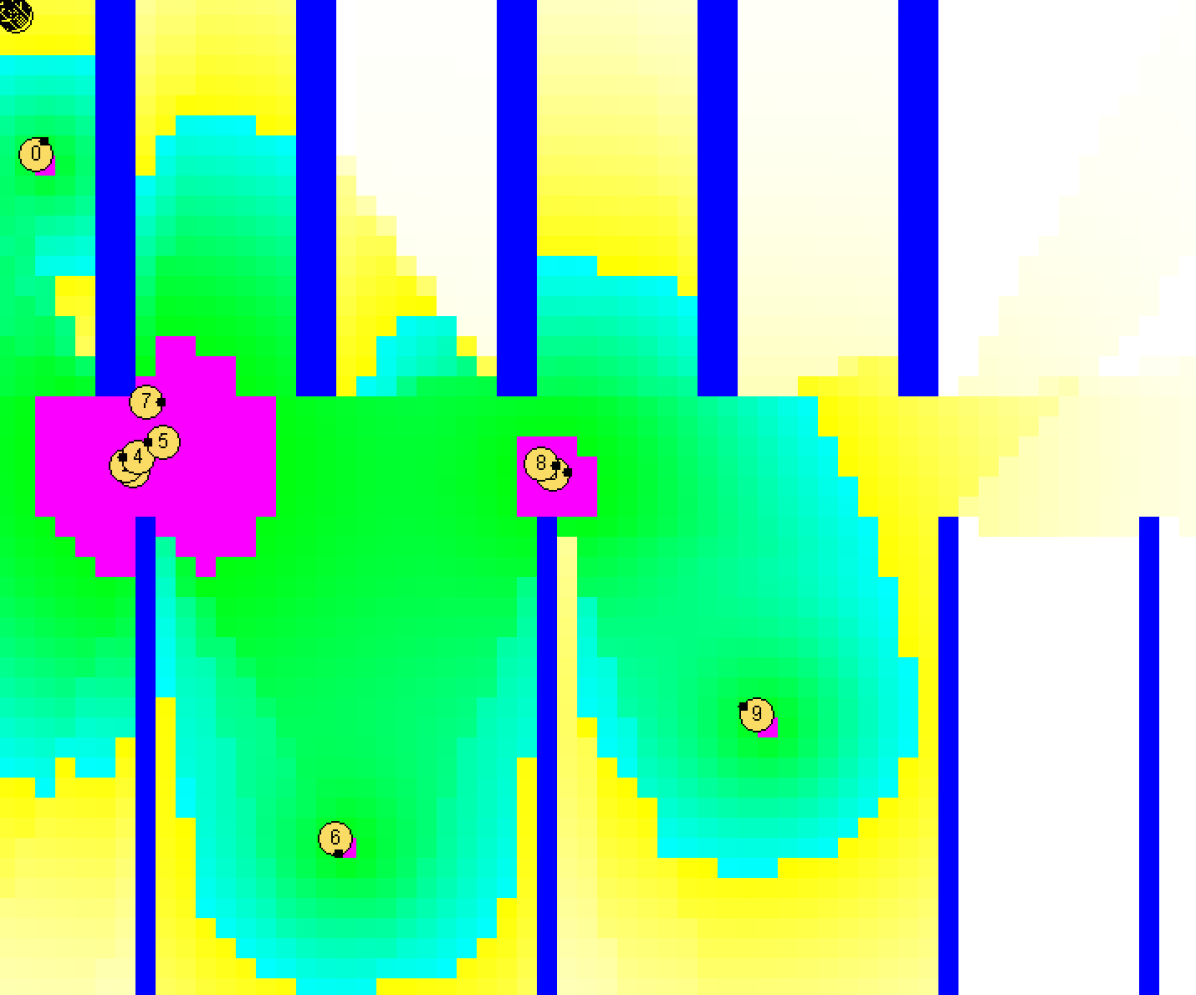
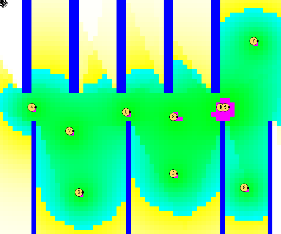
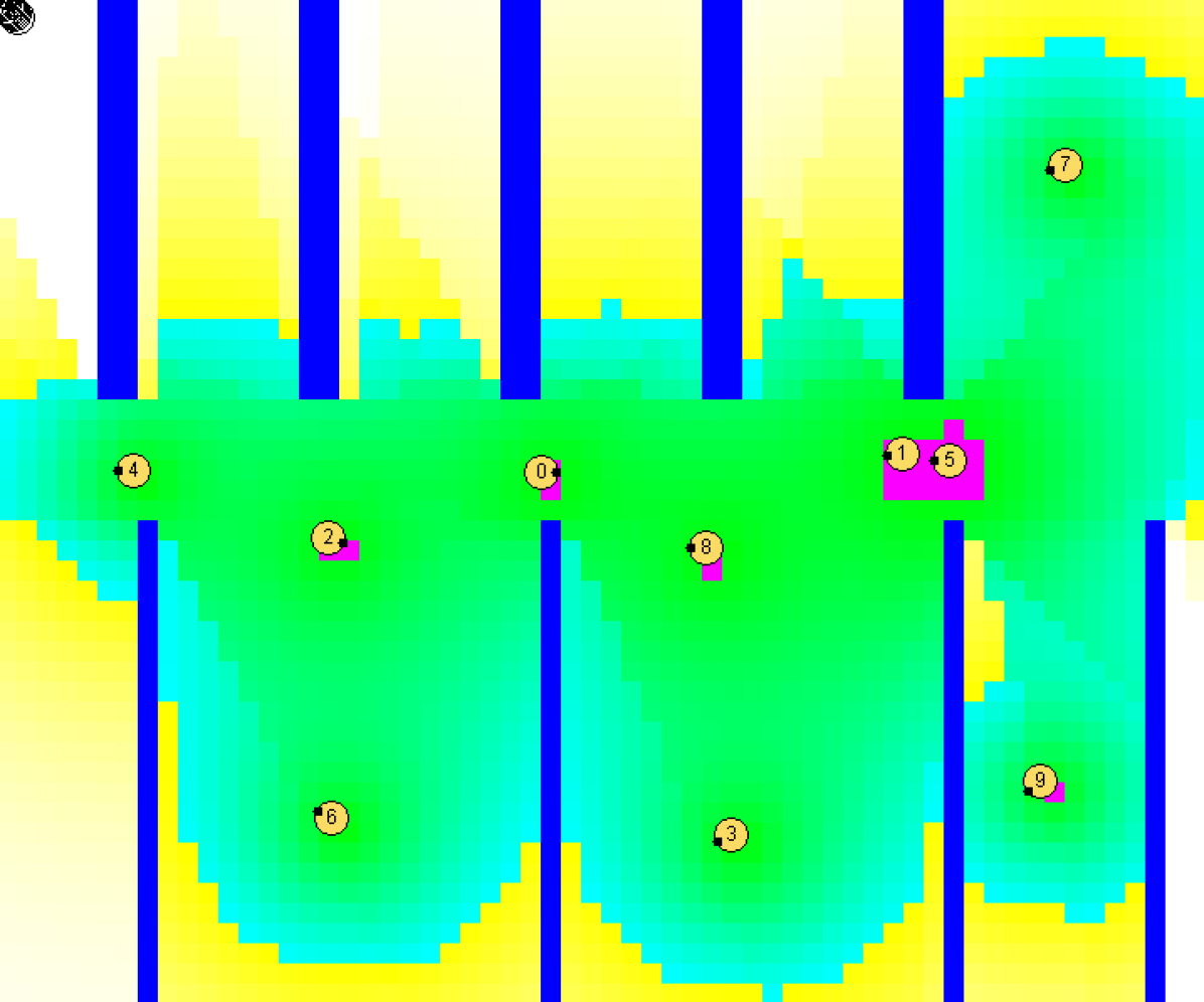
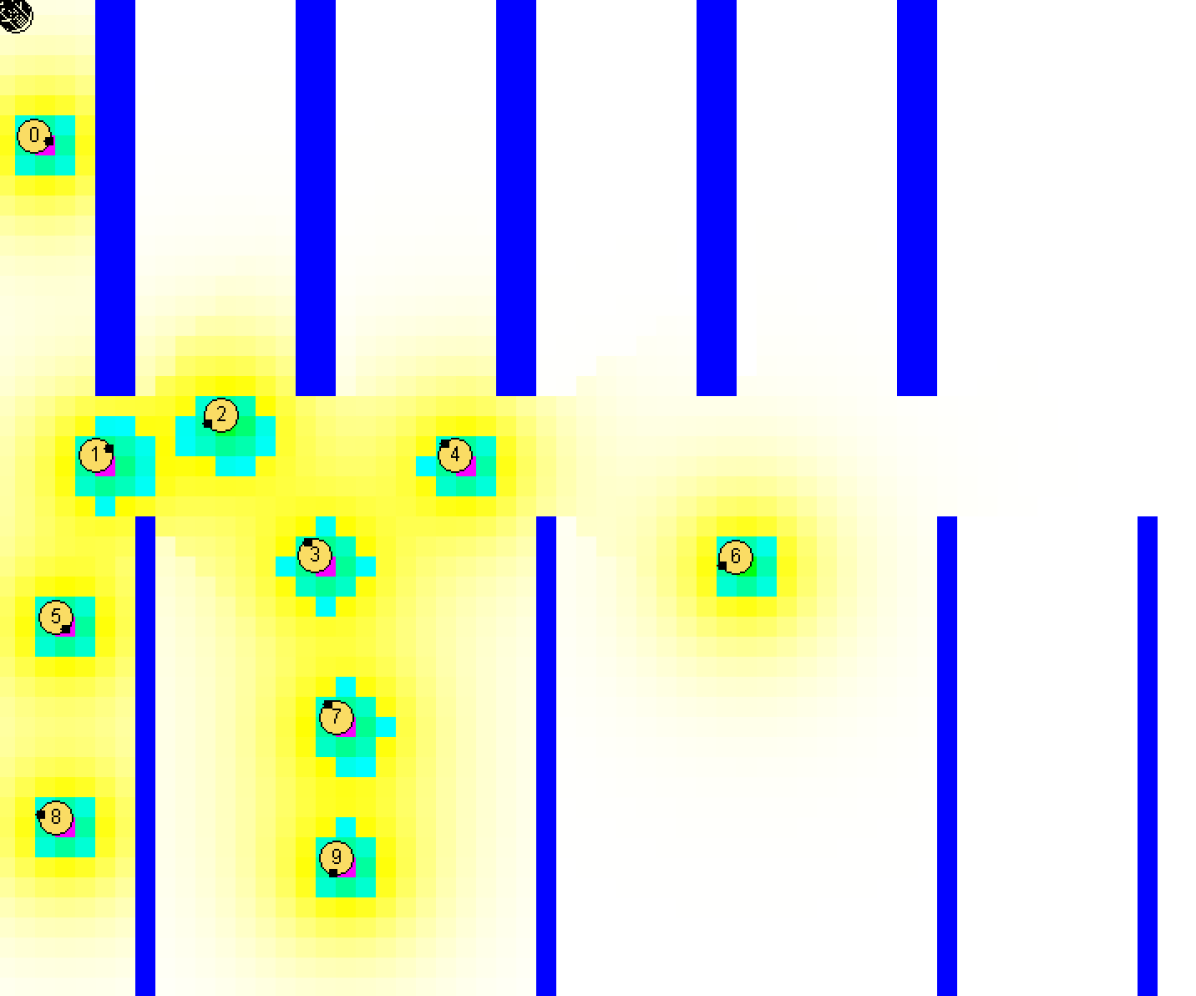
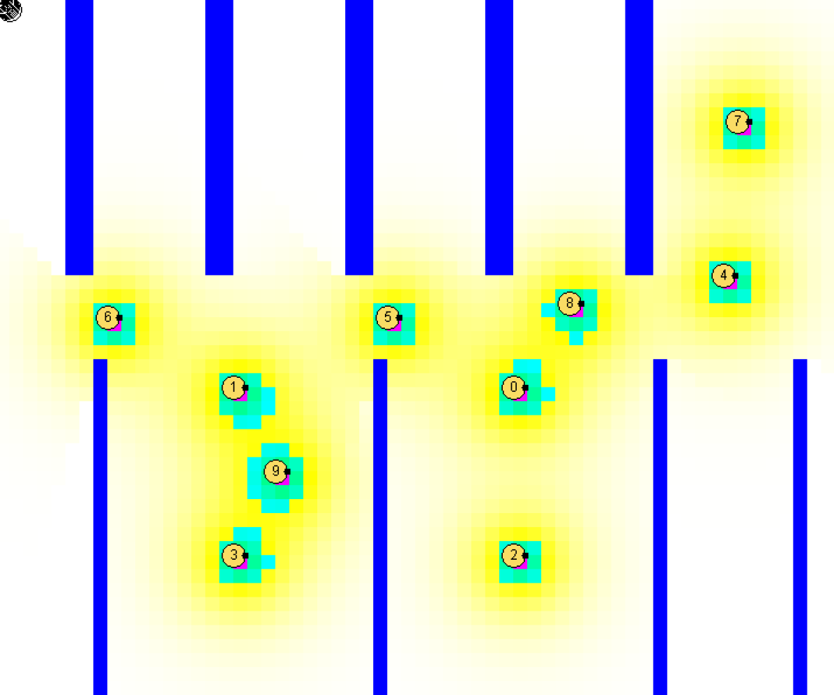
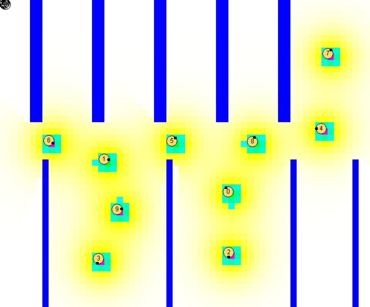
Next, we compare the performance of the greedy algorithm (Algorithm 1), the proposed GGA (Algorithm 2) and the distributed gradient algorithm in (25) for solving the optimal coverage problem in different mission spaces: no obstacles, a wall-like obstacle, a maze-like obstacle, a collection of random obstacles, and a mission space resembling a building with multiple rooms. Since the global optimum is unknown, we resort to comparing all three results as shown in Figs. 5-7, Figs. 8-10, Figs. 11-13, Figs. 14-16 and Figs. 17-19 for each of these five cases. In each case, we fix the sensing range to $\delta_{i}=80,i=1,...,N$ and use three different values of $\lambda$, where (a) shows the results of our distributed gradient-based algorithm, (b) shows the results under the greedy algorithm, and (c) shows the results under the GGA. The mission space is colored from dark to light as the joint detection probability (our objective function) decreases: the joint detection probability is $\geq 0.97$ for purple areas, $\geq 0.50$ for green areas, and near zero for white areas.

When there are no obstacles, all algorithms perform similarly, as shown in Figs. 5-7, although the actual agent configurations are generally different (suggesting that there are multiple equivalent local, and possibly global, optima.) For the case where $\lambda=0.02$, the greedy algorithm is guaranteed to be within about $8\%$ of the global optimum of (4) (using Fig. 3) and we see that using the GGA hardly improves performance, probably because the actual global optimum is achieved.

For all cases with obstacles in the mission space, the greedy algorithm and the GGA clearly outperform the basic gradient-based algorithm. Moreover, the results of the GGA significantly improve upon those reported in our previous work [10]. As an example, in the cases of Figs. 17-19 with $\lambda=0.12$, the objective function value is improved from a value of $1419.5$ reported in [10] (using the distributed gradient-based algorithm with improvements provided through the use of boosting functions) to $1466.9$ using the GGA as shown in Fig. 18.

(a) $H(\textbf{s})=2999.7$

(b) $H(\textbf{s})=2999.6$

(c) $H(\textbf{s})=2999.7$

Figure 5: The decay factor $\lambda=0.02$, and no obstacles in the mission space

(a) $H(\textbf{s})=2105.3$

(b) $H(\textbf{s})=2080.9$

(c) $H(\textbf{s})=2105.3$

Figure 6: The decay factor $\lambda=0.12$, and no obstacles in the mission space

(a) $H(\textbf{s})=78.3$

(b) $H(\textbf{s})=78.3$

(c) $H(\textbf{s})=78.3$

Figure 7: The decay factor $\lambda=0.4$, and no obstacles in the mission space

(a) $H(\textbf{s})=2771.3$

(b) $H(\textbf{s})=2773.9$

(c) $H(\textbf{s})=2774.6$

Figure 8: The decay factor $\lambda=0.02$, and a wall-like obstacle in the mission space

(a) $H(\textbf{s})=437.1$

(b) $H(\textbf{s})=1813.3$

(c) $H(\textbf{s})=1846.3$

Figure 9: The decay factor $\lambda=0.12$, and a wall-like obstacle in the mission space

(a) $H(\textbf{s})=269.6$

(b) $H(\textbf{s})=371.9$

(c) $H(\textbf{s})=373.2$

Figure 10: The decay factor $\lambda=0.4$, and a wall-like obstacle in the mission space

(a) $H(\textbf{s})=2401.6$

(b) $H(\textbf{s})=2421.9$

(c) $H(\textbf{s})=2423.4$

Figure 11: The decay factor $\lambda=0.02$, in a general mission space

(a) $H(\textbf{s})=1443.4$

(b) $H(\textbf{s})=1518.9$

(c) $H(\textbf{s})=1532.9$

Figure 12: The decay factor $\lambda=0.12$, in a general mission space

(a) $H(\textbf{s})=325.8$

(b) $H(\textbf{s})=349.2$

(c) $H(\textbf{s})=349.4$

Figure 13: The decay factor $\lambda=0.4$, in a general mission space

(a) $H(\textbf{s})=1792.2$

(b) $H(\textbf{s})=2490.0$

(c) $H(\textbf{s})=2490.6$

Figure 14: The decay factor $\lambda=0.02$, in a maze mission space

(a) $H(\textbf{s})=924.5$

(b) $H(\textbf{s})=1297.6$

(c) $H(\textbf{s})=1307.9$

Figure 15: The decay factor $\lambda=0.12$, in a maze mission space

(a) $H(\textbf{s})=275.0$

(b) $H(\textbf{s})=311.1$

(c) $H(\textbf{s})=311.1$

Figure 16: The decay factor $\lambda=0.4$, in a maze mission space

(a) $H(\textbf{s})=2418.8$

(b) $H(\textbf{s})=2582.3$

(c) $H(\textbf{s})=2583.5$

Figure 17: The decay factor $\lambda=0.02$, in a room mission space

(a) $H(\textbf{s})=1187.0$

(b) $H(\textbf{s})=1462.6$

(c) $H(\textbf{s})=1466.9$

Figure 18: The decay factor $\lambda=0.12$, in a room mission space

(a) $H(\textbf{s})=303.1$

(b) $H(\textbf{s})=344.5$

(c) $H(\textbf{s})=347.2$

Figure 19: The decay factor $\lambda=0.4$, in a room mission space

VI CONCLUSION AND FUTURE WORK

We have obtained a solution to the optimal coverage problem through the greedy algorithm (whose time complexity is linear in the number of agents in the network) with a guaranteed lower bound relative to the global optimum which is significantly tighter than the one well-known in the literature to be $1-1/e$. This is made possible by proving that our coverage metric is monotone submodular and by calculating its total curvature and its elemental curvature. Therefore, we are able to reduce the theoretical performance gap between optimal and suboptimal solutions enabled by the submodularity theory. Moreover, we have shown that the two new bounds derived are complementary with respect to the sensing capabilities of the agents and each one approaches its maximal value of 1 under different conditions on the sensing capabilities, enabling us to select the most appropriate one depending on the characteristics of the agents at our disposal. In addition, by combining the greedy algorithm with a distributed gradient-based algorithm we have proposed a greedy-gradient algorithm (GGA) so as to improve the coverage performance by searching in a continuous feasible region with initial conditions provided by the greedy algorithm. We have included simulation results uniformly showing that the proposed distributed GGA outperforms other related methods we are aware of.

An interesting future research direction is to study whether a distributed greedy algorithm can be developed and whether the lower bounds obtained through the associated curvatures are still as tight as those we have obtained so far.

Appendix A Proof of Equivalence

Definition 1 $\Rightarrow$ Definition 2

Suppose that $S\subseteq T$, $y\notin T$, and $f$ satisfies (5). Replacing $S$ in (5) by $S\cup\left\{y\right\}$ gives

$$f(S\cup\left\{y\right\}\cup T)+f(S\cup\left\{y\right\}\cap T)\leq f(S\cup\left\{y\right\})+f(T).$$ (26)

Rearranging the terms in (26), we obtain (6).

Definition 2 $\Rightarrow$ Definition 1

Suppose that $f$ satisfies (6), and $y\in S/(S\cap T)$. It is easy to verify that $S\cap T\subseteq T$, and $y\notin T$. Replacing $S$ in (6) by $S\cap T$, and using (6) repeatedly to all elements $y\in S/(S\cap T)$, we obtain

$$\begin{split}&\underset{f\left(S\right)}{\underbrace{f\left(S\cap T\cup(S/(S\cap T))\right)}}-f\left(S\cap T\right)\\ &\qquad\qquad\qquad\geq\underset{f\left(T\cup S\right)}{\underbrace{f\left(T\cup(S/(S\cap T))\right)}}-f\left(T\right).\end{split}$$ (27)

Rearranging the terms in (LABEL:appe2) gives (5).

References

- [1] S. Meguerdichian, F. Koushanfar, M. Potkonjak, and M. B. Srivastava, “Coverage problems in wireless ad-hoc sensor networks,” in Proc. 20th Joint Conf. of the IEEE Computer and Commun. Societies, vol. 3, 2001, pp. 1380–1387.
- [2] C. G. Cassandras and W. Li, “Sensor networks and cooperative control,” European J. of Control, vol. 11, no. 4-5, pp. 436–463, 2005.
- [3] C. Caicedo-Nuez and M. Zefran, “A coverage algorithm for a class of non-convex regions,” in Proc. 47th IEEE Conf. on Decision and Control, 2008, pp. 4244–4249.
- [4] C. H. Caicedo-Nunez and M. Zefran, “Performing coverage on nonconvex domains,” in Proc. IEEE Conf. on Control Applic., 2008, pp. 1019–1024.
- [5] A. Breitenmoser, M. Schwager, J.-C. Metzger, R. Siegwart, and D. Rus, “Voronoi coverage of non-convex environments with a group of networked robots,” in Proc. IEEE Int. Conf. on Robotics and Automation, 2010, pp. 4982–4989.
- [6] M. Zhong and C. G. Cassandras, “Distributed coverage control and data collection with mobile sensor networks,” IEEE Trans. on Automatic Control, vol. 56, no. 10, pp. 2445–2455, 2011.
- [7] A. Gusrialdi and L. Zeng, “Distributed deployment algorithms for robotic visual sensor networks in non-convex environment,” in Networking, Sensing and Control (ICNSC), 2011 IEEE International Conference on. IEEE, 2011, pp. 445–450.
- [8] J. Cortes, S. Martinez, T. Karatas, and F. Bullo, “Coverage control for mobile sensing networks,” IEEE Trans. on Robotics and Automation, vol. 20, no. 2, pp. 243–255, 2004.
- [9] A. Gusrialdi, S. Hirche, T. Hatanaka, and M. Fujita, “Voronoi based coverage control with anisotropic sensors,” in Proc. American Control Conf., 2008, pp. 736–741.
- [10] X. Sun, C. G. Cassandras, and K. Gokbayrak, “Escaping local optima in a class of multi-agent distributed optimization problems: A boosting function approach,” in Decision and Control (CDC), 2014 IEEE 53rd Annual Conference on. IEEE, 2014, pp. 3701–3706.
- [11] M. Schwager, F. Bullo, D. Skelly, and D. Rus, “A ladybug exploration strategy for distributed adaptive coverage control,” in Proc. IEEE Int. Conf. on Robotics and Automation, 2008, pp. 2346–2353.
- [12] P. J. Van Laarhoven and E. H. Aarts, Simulated annealing. Springer, 1987.
- [13] D. Bertsimas and J. Tsitsiklis, “Simulated annealing,” Statistical Science, pp. 10–15, 1993.
- [14] S. Khuller, A. Moss, and J. S. Naor, “The budgeted maximum coverage problem,” Inf. Processing Letters, vol. 70, no. 1, pp. 39–45, 1999.
- [15] O. Berman and D. Krass, “The generalized maximal covering location problem,” Computers & Operations Research, vol. 29, no. 6, pp. 563–581, 2002.
- [16] G. L. Nemhauser, L. A. Wolsey, and M. L. Fisher, “An analysis of approximations for maximizing submodular set functions —I,” Mathematical Programming, vol. 14, no. 1, pp. 265–294, 1978.
- [17] A. Krause, A. Singh, and C. Guestrin, “Near-optimal sensor placements in gaussian processes: Theory, efficient algorithms and empirical studies,” J. of Machine Learning Research, vol. 9, no. Feb, pp. 235–284, 2008.
- [18] A. Krause, J. Leskovec, C. Guestrin, J. VanBriesen, and C. Faloutsos, “Efficient sensor placement optimization for securing large water distribution networks,” J. of Water Resources Planning and Management, vol. 134, no. 6, pp. 516–526, 2008.
- [19] Z. Zhang, E. K. Chong, A. Pezeshki, and W. Moran, “String submodular functions with curvature constraints,” IEEE Trans. on Automatic Control, vol. 61, no. 3, pp. 601–616, 2016.
- [20] Y. Liu, Z. Zhang, E. K. Chong, and A. Pezeshki, “Performance bounds for the k-batch greedy strategy in optimization problems with curvature,” in American Control Conference. IEEE, 2016, pp. 7177–7182.
- [21] M. Conforti and G. Cornuejols, “Submodular set functions, matroids and the greedy algorithm: tight worst-case bounds and some generalizations of the rado-edmonds theorem,” Discrete applied mathematics, vol. 7, no. 3, pp. 251–274, 1984.
- [22] Z. Wang, B. Moran, X. Wang, and Q. Pan, “Approximation for maximizing monotone non-decreasing set functions with a greedy method,” J. of Combinatorial Optimization, vol. 31, no. 1, pp. 29–43, 2016.
- [23] M. L. Fisher, G. L. Nemhauser, and L. A. Wolsey, “An analysis of approximations for maximizing submodular set functions —II,” in Polyhedral combinatorics. Springer, 1978, pp. 73–87.
- [24] D. P. Bertsekas, Nonlinear Programming. Athena Scientific, 1995.