Binary Generative Adversarial Networks for Image Retrieval
Abstract.
The most striking successes in image retrieval using deep hashing have mostly involved discriminative models, which require labels. In this paper, we use binary generative adversarial networks (BGAN) to embed images to binary codes in an unsupervised way. By restricting the input noise variable of generative adversarial networks (GAN) to be binary and conditioned on the features of each input image, BGAN can simultaneously learn a binary representation per image, and generate an image plausibly similar to the original one. In the proposed framework, we address two main problems: 1) how to directly generate binary codes without relaxation? 2) how to equip the binary representation with the ability of accurate image retrieval? We resolve these problems by proposing new sign-activation strategy and a loss function steering the learning process, which consists of new models for adversarial loss, a content loss, and a neighborhood structure loss. Experimental results on standard datasets (CIFAR-10, NUSWIDE, and Flickr) demonstrate that our BGAN significantly outperforms existing hashing methods by up to 107% in terms of mAP (See Table 3)111Our anonymous code is available at: https://github.com/htconquer/BGAN.
1. Introduction
With the rapidly increasing amount of images, similarity search in large image collections has been actively pursued in a number of domains, including computer vision, information retrieval and pattern recognition (Shakhnarovich et al., 2008; Wang et al., 2014a). However, exact nearest-neighbor (NN) search is often intractable because of the size of dataset and the high dimensionality of images. Instead, approximate nearest-neighbor (ANN) search is more practical and can achieve orders of magnitude in speed-up compared to exact NN search (Shakhnarovich et al., 2008; Jégou et al., 2011).
Recently, learning-based hashing methods (Norouzi and Fleet, 2013; Wang et al., 2014a; Irie et al., 2014; Lin et al., 2014; Hu et al., 2014; Wang et al., 2014b) have become the mainstream for scalable image retrieval due to their compact binary representation and efficient Hamming distance calculation. Such approaches embed data points to compact binary codes through hash functions, which can be generally expressed as:
| (1) |
where , are the hash functions, and b is a binary vector with code length .
Hashing methods can be generally categorized as being unsupervised or supervised. The unsupervised learning of a hash function is usually based on the criterion of preserving important properties of the training data points in the original space. Typical approaches target pairwise similarity preservation (i.e., the similarity/distance of binary codes should be consistent with that of the original data points) (Weiss et al., 2008; Liu et al., 2014a; Irie et al., 2014), multi-wise similarity preservation (i.e., the similarity orders over more than two items computed from the input space and the coding space should be preserved) (Norouzi and Fleet, 2011; Wang et al., 2013), or implicit similarity preservation (i.e., pursuing effective space partitioning without explicitly evaluating the relation between the distances/similarities in the input and coding spaces), (Heo et al., 2015; Jin et al., 2013). A fundamental limitation of a hashing method geared to preserve a particular image property is that its performance may degrade when it is is applied to a context where a different property is relevant.
Supervised hashing is designed to generate the binary codes based on predefined labels (Lin et al., 2014; Ge et al., 2014; Strecha et al., 2012). For example, Strecha et al. (Strecha et al., 2012) developed a supervised hashing which maximizes the between-class Hamming distance and minimizes the within-class Hamming distance. (Lin et al., 2014; Ge et al., 2014) proposed to learn the hash codes such to approximate the pairwise label similarity. Supervised hashing methods usually significantly outperform unsupervised methods. However, the information that can be used for supervision is also typically scarce.
More recently, deep learning has been introduced in the development of hashing algorithms (Rongkai Xia and Yan, 2014; Guo et al., 2016; Dai et al., 2016; Lin et al., 2016; Do et al., 2016; Yang et al., 2017; Gu et al., 2016), leading to a new generation of deep hashing algorithms. Due to powerful feature representation, remarkable image retrieval performance has been reported using the hashes obtained in this way. However, a number of open issues have still remain open. The most successful deep hashing methods are usually supervised and require labels. The labels are, however, scarce and subjective. Unsupervised approaches, on the other hand, cannot take full advantages of the current deep learning models, and thus yield unsatisfactory performance (Lin et al., 2016). Another issue is a non-smooth sign-activation function used to generate the binary codes, which, despite several ideas proposed to tackle it (Li et al., 2015; Cao et al., 2017; Do et al., 2016), still makes the standard back-propagation infeasible.
To address the above issues, we propose an unsupervised hashing method that deploys a generative adversarial network (GAN) (Reed et al., 2016). GAN has proven effective to generate synthetic data similar to the training data from a latent space. Therefore, if we restrict the input noise variable of generative adversarial networks (GAN) to be binary and conditioned on the features of each input image, we can learn a binary representation for each image and generate a plausibly similar image to the original one simultaneously. Feeding the generated images through a “discriminator” that verifies them with respect to the training images removes the need for supervision and the relevant hash can be learned in an unsupervised fashion. We refer to this proposed architecture as binary GAN (BGAN). For the BGAN learning process, we design a novel loss function to equip the binary representation with the ability of accurate image retrieval, beyond vivid image generation. Furthermore, inspired by recent studies on continuation methods (Allgower and Georg, 2012; Cao et al., 2017), we propose two equivalent realizations of the sign-activation function, and design an optimization strategy whose solution is equivalent to the non-smooth sign function.
2. Related Work
2.1. Hashing
Existing hashing methods can be generally divided into two categories: unsupervised, and supervised methods. For unsupervised methods (Gong et al., 2013a; Salakhutdinov and Hinton, 2009; Dai et al., 2016; Lin et al., 2016; Erin Liong et al., 2015), label information is not required in the learning process. For example, Lin et al. (Lin et al., 2016) proposed an unsupervised deep learning approach, DeepBit, imposing three criteria on binary codes (i.e., minimal loss quantization, evenly distributed codes and uncorrelated bits) to learn a compact binary descriptor for efficient visual object matching. The ITQ method proposed by Gong et al. (Gong et al., 2013a) maximizes the variance of each binary bit and minimizes the binarization loss to obtain a high performance for image retrieval. Liong et.al (Erin Liong et al., 2015) proposed to use a deep neural network to learn hash codes by optimizing for three objectives: (1) the loss between the real-valued feature descriptor and the learned binary codes is minimized, (2) binary codes distribute evenly on each bit and (3) different bits are as independent as possible.
Supervised hashing methods (Rongkai Xia and Yan, 2014; Guo et al., 2016; Do et al., 2016; Li et al., 2015; Yang et al., 2017; Gu et al., 2016) utilize the label information and can usually obtain better performance. Most of the methods apply pairwise label loss as criterion for optimization. An example is the deep supervised hashing method by Li et.al (Li et al., 2015), which can simultaneously learn features and hash codes. Another example is Supervised Recurrent Hashing (SRH) for creating video hashes, as proposed by Gu et. al. (Gu et al., 2016). Cao et.al (Cao et al., 2017) proposed a continuous method to learn binary codes, which can avoid the relaxation of binary constraints (Gu et al., 2016) by first learning continuous representations and then thresholding them to get the hash codes. They also added weight to data for balancing similar and dissimilar pairs.
So far, only supervised hashing methods have been reasonably successful in benefiting from the effectiveness of deep learning. In this paper we address the challenge of enabling an unsupervised method to also take full advantage of this machine learning approach and generate reliable hash codes without the need for class labels.
We also address a specific issue related to the deployment of a deep learning approach in the hashing context, namely that a non-smooth sign-activation function used to generate the binary codes still makes the standard back-propagation infeasible. With our new proposed sign-activation strategy, we provide an effective alternative to earlier attempts to address this issue (Li et al., 2015; Cao et al., 2017; Do et al., 2016). For instance, in (Cao et al., 2017), Cao et. al. proposed a tanh-like function to replace the sign activation and Li et. al. introduced an intermediate continuous variable to approximate the binary code (Li et al., 2015; Do et al., 2016). Essentially, they relaxed the binary constraints and the binary codes were further generated by a sign function. Furthermore, the work of Cao et. al. (Cao et al., 2017) only considered a special case of solving the non-smooth sign function, instead of looking for a generalized solution.
2.2. Generative Adversarial Nets
Ian et. al. (Goodfellow et al., 2014) proposed Generative Adversarial Network (GAN), which has been widely applied in computer vision and natural language processing. In the nutshell, GAN is an architecture for playing a min-max game, where two competing processes aim at maximizing their individual, but mutually conflicting, objectives. GAN has shown its effectiveness in various application contexts and various variants of the original GAN concept have been developed (Radford et al., 2015; Larsen et al., 2015; Chen et al., 2016). Radford et. al. (Radford et al., 2015) proposed a method for unsupervised feature learning using deep convolutional generative adversarial networks (DCGAN), which was shown to be superior to other unsupervised algorithms. In (Larsen et al., 2015), Larsen et. al. combined a variational autoencoder (VAE) (Kingma and Welling, 2013) and GAN to use learned feature representations in the GAN discriminator as the basis for the VAE reconstruction objective. This approach was shown to outperform VAEs with element-wise similarity measures in terms of visual fidelity. In (Chen et al., 2016), Chen et. al. proposed a model called Variational InfoGAN (ViGAN), which not only can generate new images based on visual descriptions, but can also retain the latent representation of an image and varying the visual description.
Nevertheless, the learned representations serving as input into the GAN generator in the above methods are not binary. Using a binary image representation in combination with a GAN framework is a new challenge that we address in this paper by proposing binary generative adversarial networks (BGAN).
3. Binary Generative Adversarial Networks
Given images, without labels, our goal is to learn their compact binary codes B and reconstructed images for the original images such that: (a) the binary codes can reconstruct the image content, and (b) the binary codes could be computed directly without relaxation.
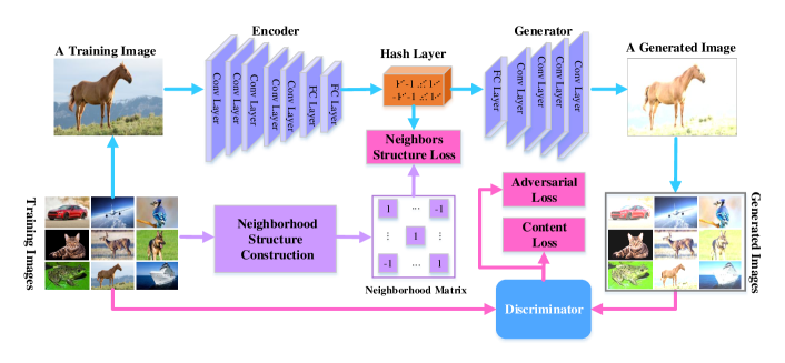
We illustrate our proposed BGAN architecture by the scheme in Fig. 1. The scheme shows how hash codes are learned in an unsupervised fashion through the interplay between, on the one side, the image generation process (the generator module) taking the generated hash code (the hash layer) as input, and, on the other side, the verification process (the discriminator module) where the images from the generator are compared to the original training images. For training of the system, we first construct the neighborhood structure of images and then train the neural network underlying the encoder, generator and discriminator. In the remainder of this section, we describe the process of constructing the neighborhood structure, the network architecture, our loss function and learning of parameters.
3.1. Construction of Neighborhood Structure
In our unsupervised approach, we propose to exploit the neighborhood structure of the images in a feature space as information source steering the process of hash learning. Specifically, we propose a method based on the K-Nearest Neighbor (KNN) concept to create a neighborhood matrix S. Based on (He et al., 2015), we extract 2,048-dimensional features from the pool5-layer. This results in the set where is the feature vector of image .
For the representation of the neighboring structure, our task is to construct a matrix , whose elements indicate the similarity () or dissimilarity () of any two images and in terms of their features and .
We compare images using cosine similarity of the feature vectors. For each image, we select images with the highest cosine similarity as its neighbors. Then we can construct an initial similarity matrix :
| (4) |
The precision curve (evaluated using the labels) in Figure 2 indicates the quality of the constructed neighborhood for different values of . Due to rapidly decreasing precision with increasing , creating a large-enough neighborhood by simply increasing is not the best option. In order to find a better approach, we borrow the ideas from the domain of graph modeling. In an undirected graph, if a node is connected to a node and if is connected to a node , we can infer that is also connected to . Inspired by this, if we treat every training image as a node in an undirected graph, we can expand the neighborhood of an image by exploring the neighbors of its neighbors. Specifically, if connects to and connects to , we can infer that has the potential to be also connected to .
In view of the above, we use the initial similarity matrix to expand the neighborhood structure. Specifically, based on , we calculate the similarity of two images by comparing the corresponding columns in using the expression . Then we again construct a ranked list of neighbors, based on which we generate the second similarity matrix as:
| (7) |
Finally, we construct the neighborhood structure by combining the direct and indirect similarities from the two matrices together. This results in the final similarity matrix S:
| (10) |
The whole algorithm is shown in Alg. 1. We note here that we could have also omitted this preprocessing step and construct the neighborhood structure directly during the learning of our neural network. We found, however, that the construction of neighborhood structure is time-consuming, and that updating of this structure based on the updating of image features in each epoch does not have significant impact on the performance. Therefore, we chose to obtain this neighborhood structure as described above and fix it for the rest of the process.
3.2. Architecture Structure
As shown in Figure 1, our proposed BGAN consists of four components: encoder, hashing, generator and discriminator. We describe each of them in detail in the remainder of this section.
3.2.1. Encoder
For feature extraction, we use a structure similar to VGG19 (Szegedy et al., 2015), with the details shown in table 1. We use 5 groups of convolution layers and 5 max convolution-pooling layers. Similar to (Szegedy et al., 2015), we use 64, 128, 256, 512, 512 filters in the 5 groups of convolutional layers, respectively.
| Layer | Size of Filter | Number of Filters | Others |
| conv1_1 | 3x3 | 64 | Stride=1,padding=1,relu |
| conv1_2 | 3x3 | 64 | Stride=1,padding=1,relu |
| Max pooling | 2x2 | 2 | |
| conv2_1 | 3x3 | 128 | Stride=1,padding=1,relu |
| conv2_2 | 3x3 | 128 | Stride=1,padding=1,relu |
| Max pooling | 2x2 | 2 | |
| conv3_1 | 3x3 | 256 | Stride=1,padding=1,relu |
| conv3_2 | 3x3 | 256 | Stride=1,padding=1,relu |
| conv3_3 | 3x3 | 256 | Stride=1,padding=1,relu |
| Max pooling | 2x2 | 2 | |
| conv4_1 | 3x3 | 512 | Stride=1,padding=1,relu |
| conv4_2 | 3x3 | 512 | Stride=1,padding=1,relu |
| conv4_3 | 3x3 | 512 | Stride=1,padding=1,relu |
| Max pooling | 2x2 | 2 | |
| conv5_1 | 3x3 | 512 | Stride=1,padding=1,relu |
| conv5_2 | 3x3 | 512 | Stride=1,padding=1,relu |
| conv5_3 | 3x3 | 512 | Stride=1,padding=1,relu |
| Max pooling | 2x2 | 2 | |
| FC6 | 4096 | relu | |
| FC7 | 4096 | relu |
3.2.2. Hashing
A binary hash code is learned directly, by converting the -dimensional representation z learned from the last fully-connected layer FC7, which is continuous in nature, to a binary hash code b taking values of either or . This binarization process can only be performed by taking the sign function as the activation function on top of the hash layer.
Unfortunately, as the sign function is non-smooth and non-convex, its gradient is zero for all nonzero inputs, and is ill-defined at zero, which makes the standard back-propagation infeasible for training deep networks. This is known as the vanishing gradient problem, which has been a key difficulty in training deep neural networks via back-propagation [14]. Approximate solutions (Zhang et al., 2014; Kang et al., 2016) that relax the binary constraints are not a good alternative as they lead to a large quantization error and thereofre to a suboptimal solution (Zhang et al., 2014).
In order to tackle this challenge of optimizing deep networks with non-smooth sign activation, we draw inspiration from recent studies on continuation methods (Allgower and Georg, 2012; Cao et al., 2017). These studies address a complex optimization problem by smoothing the original function, turning it into a different problem that is easier to optimize. By gradually reducing the amount of smoothing during the training, this results in a sequence of optimization problems converging to the original optimization problem. Following this approach, if we find an approximate smooth function of , and then gradually make the smoothed objective function non-smooth as the training proceeds, the final solution should converge to the desired optimization target.
Motivated by the continuation methods, we define a function to approximate :
| (14) |
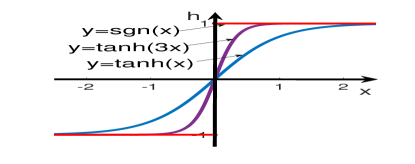
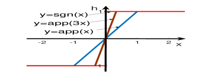
We notice that there exists a key relationship between the sign function and the app function in the concept of limit:
| (15) |
An illustration of the process through which approximates is given in Fig. 3. The figure also shows the same process for an alternative to : :
| (16) |
3.2.3. Generator and Discriminator
The task of our BGAN “Generator” network G is to generate an image based on the hash code b. First, we let b serve as the input of the top fully-connected layer with the size . Then, we use four deconvolutional layers with the size of kernels , and the number of kernels , which is followed by batch-normalization layers and eLU as the activation function.
Following the approach by Goodfellow et al. (Goodfellow et al., 2014), we define a “Discriminator” network D in such a way that it is optimized using criteria that are conflicting to those of G. In this way, D can act as adversary to G in the overall min-max optimization process. The goal of this optimization is to improve G such to be able to generate the images as well as possible. The process being adversarial to image generation is the process of trying to distinguish between the original and reconstructed images. If G manages to generate the images so well to “fool” D, then it “wins” the min-max game and the overall GAN optimization has converged. In view of this, given a model of the image classifier D assessing the original (I) and reconstructed () image, we can formally define the min-max game resulting in the optimal system parameters as follows:
| (17) |
Here we follow the architecture design summarized by Radford et al. (Radford et al., 2015), use eLU activation and avoid max-pooling throughout the network. It contains 4 convolutional layers with an increasing number of filter kernels (32, 128, 256, and 512). Strided convolutions are used to reduce the image resolution each time the number of features is doubled. The resulting 512 feature maps are followed by a dense layer with the size of 1024 and a final sigmoid activation function to obtain a probability for sample classification.
3.3. Loss Function
The definition of the loss function is critical for the performance of our network as it steers the overall optimization of the min-max game. While auto-encoding is commonly modeled based on the Mean Squared Error, we follow (Larsen et al., 2015; Ledig et al., 2016) and design a loss function that assesses our hashing solution with respect to perceptually relevant characteristics. We formulate the loss function as the weighted sum of a neighbor structure loss, content loss and adversarial loss as:
| (18) |
In the following subsections, we explain our realization of each of the loss functions.
3.3.1. Neighbors Structure Loss
The neighborhood structure loss models the loss in the similarity structure in data, as revealed in the set of neighbors obtained for an image by applying the hash code of that image. Given the binary codes for all the images of the length , and using the similarity matrix S as the reference for similarity relations between images, we define the neighbors structure loss as follows:
| (19) |
The goal of optimizing for this loss function is clearly to bring the binary codes of similar images as close to each other as possible.
3.3.2. Content Loss
The content loss models the loss in the quality of reconstructed images. The most widely used pixel-wise MSE loss is calculated as:
| (20) |
However, as pointed out in (Ledig et al., 2016), solutions of MSE optimization problems often lack high-frequency content, which results in perceptually unsatisfying solutions with overly smooth textures. Also, element-wise reconstruction errors are not robust for images and other signals with invariance.
Therefore, instead of only relying on pixel-wise losses we build on the ideas of Christian et. al. (Ledig et al., 2016) and use a loss function that closer resembles perceptual similarity. Specifically, we define the VGG loss based on the eLU activation layers of the last convolutional layer of our discriminator networks D. With we indicate the feature map obtained by the last convolution (after activation) and then define the VGG loss as the Euclidean distance between the feature representations of a reconstructed image and the original image :
| (21) |
Here, and represent the dimensions of the respective feature maps. Based on the above, we can now define the content loss as:
| (22) |
3.3.3. Adversarial Loss:
The adversarial loss models the loss due to misclassification of images, as done by D, in the original and reconstructed ones. Using the notations already explained in the context of Eq.8, we model this loss as:
| (23) |
3.4. Learning
Using the loss function in Eq.18, we train our network. The forward propagation is as follows. First, we use a deep convolutional network as the encoder to extract the features and then use hash layer to obtain to embed the real-valued features into binary codes:
| (24) |
where is an input image, is the parameter of the encoder and stands for the parameter of generating Z. Then, is the input for a generator G to reconstruct an image :
| (25) |
where stands for the parameters of the generator G. Finally, a discriminator assigns probability:
| (26) |
that is an actual training sample and probability that is generated by our model .
In the network, we have parameters of , , and to learn. We use back-propagation (BP) for learning and stochastic gradient descent (SGD) to minimize the loss. In particular, we initialize network parameters and use forward propagation to obtain the value of each loss (). In each iteration, we sample a mini-batch of images from the training set, and then update each parameter:
| (27) | |||
| (28) | |||
| (29) | |||
| (30) |
where is the learning rate. We train our network until it converges.
For the hashing layer, we start training BGAN with . For each stage , after BGAN converges, we increase and train (i.e., fine-tune) BGAN by setting the converged network parameters as the initialization for training the BGAN in the next stage. By evolving with , the network will converge to BGAN with as activation function, which can generate exactly binary hash codes as we desire. Using we can already achieve fast convergence for training BGAN.
4. Experiments
We evaluate our BGAN on the task of large-scale image retrieval.
Specifically, the experiments are designed to study the following research questions of our algorithm:
RQ1: How does each component of our algorithm affect the performance?
RQ2: Does the binary codes computed directly without relaxation improve the performance of the relaxed resolution?
RQ3: Does the performance of BGAN significantly outperform the state-of-the-art hashing algorithms?
RQ4: What is the efficiency of BGAN?
4.1. Settings
4.1.1. Datasets
We conduct empirical evaluation on three public benchmark datasets, CIFAR-10, NUS-WIDE, and Flickr.
CIFAR-10 labeled subsets of the 80 million tiny images dataset, which consists of 60,000 color images in 10 classes, with 6,000 images per class.
NUS-WIDE is a web image dataset containing 269,648 images downloaded from Flickr. Tagging ground-truth for 81 semantic concepts is provided for evaluation. We follow the settings in (Zhu
et al., 2016) and use the subset of 195,834 images from the 21 most frequent concepts, where each concept consists of at least 5,000 images.
Flickr is a collection of 25,000 images from Flickr, where each image is labeled with one of the 38 concepts. We resize images of this subset into .
In NUS-WIDE and CIFAR-10, we randomly select 100 images per class as the test query set, and 1,000 images per class as the training set. In Flickr, we randomly select 1,000 images as the test query set, and 4,000 images as the training set.
4.1.2. Evaluation Metric
Hamming ranking is used as the search protocol to evaluate our proposed approaches, and two indicators are reported. 1) Mean Average Precision (mAP): For a single query, Average Precision (AP) is the average of the precision value obtained for the set of top-k results, and this value is then averaged over all the queries.2) Precision: We further use precision-recall curve and precision@K to evaluate the precision of retrieved images at each stage.
4.1.3. Compared algorithms
We compare our BGAN with other state-of-the-art hashing algorithms. Specifically, we compare with four non-deep hashing methods (iterative quantization (ITQ) hashing (Gong et al., 2013b), spectral hashing (SH) (Weiss et al., 2008), Locality Sensitive Hashing (LSH) (Datar et al., 2004) and spherical hashing (Heo et al., 2015)), and two deep hashing methods (DeepBit (Lin et al., 2016) and Deep Hashing (DH) (Erin Liong et al., 2015)).
To make a fair comparison, we also apply the non-deep hashing methods on deep features extracted by the CNN-F of the feature learning part in our BGAN. For non-deep hashing algorithms, we use 1134-D concatenated features as the hand-crafted features, including 64-D color histogram, 144-D color correlogram, 73-D edge direction histogram, 128-D wavelet texture, 225-D block-wise color moments and 500-D bag of words based on SIFT descriptions.
We also conduct the non-deep hashing methods on deep features extracted by the VGG network (VGG-fc7 (Szegedy et al., 2015)). For non-deep hashing algorithms, we use 512-dim GIST features as the hand-crafted features. We also compare with PCAH (Wang et al., 2012), DGH (Liu et al., 2014b), AGH (Liu et al., 2011), and UN-BDNH (Do et al., 2016) in term of precision.
By constructing the neighborhood structure using the labels, our method can be easily modified as a supervised hashing method. Therefore, we also compare with some supervised hashing methods, e.g., iterative quantization hashing (ITQ-CCA) (Gong et al., 2013b), KSH (Liu et al., 2012), minimal loss hashing (MLH) (Norouzi and Fleet, 2011), DNNH (Lai et al., 2015), CNNH (Rongkai Xia and Yan, 2014) and Deep Hashing Network (DHN) (Zhu et al., 2016).
4.1.4. Implementation Details
In the construction of neighborhood structure step, we set for CIFAR-10 dataset, and the average number of the neighbors for each image is for the three datasets. By default, we set and . We set the mini-batch size as 256, and the learning rate as .
4.2. Component Analysis (RQ1)
| mAP | |||
|---|---|---|---|
| Components | 24-bit | 32-bit | 48-bit |
| 0.487 | 0.511 | 0.543 | |
| - | - | - | |
| - | - | - | |
| 0.247 | 0.379 | 0.497 | |
| 0.472 | 0.503 | 0.534 | |
| - | - | - | |
| 0.512 | 0.531 | 0.558 | |
| Method | CIFAR-10 | NUS-WIDE | Flickr | |||||||||
|---|---|---|---|---|---|---|---|---|---|---|---|---|
| 12 bits | 24 bits | 32 bits | 48 bits | 12 bits | 24 bits | 32 bits | 48 bits | 12 bits | 24 bits | 32 bits | 48 bits | |
| ITQ (Gong et al., 2013b) | 0.162 | 0.169 | 0.172 | 0.175 | 0.452 | 0.468 | 0.472 | 0.477 | 0.544 | 0.555 | 0.560 | 0.570 |
| SH (Weiss et al., 2008) | 0.131 | 0.135 | 0.133 | 0.130 | 0.433 | 0.426 | 0.426 | 0.423 | 0.531 | 0.533 | 0.531 | 0.529 |
| LSH (Datar et al., 2004) | 0.121 | 0.126 | 0.120 | 0.120 | 0.403 | 0.421 | 0.426 | 0.441 | 0.499 | 0.513 | 0.521 | 0.548 |
| Spherical (Heo et al., 2015)) | 0.138 | 0.141 | 0.146 | 0.150 | 0.413 | 0.413 | 0.424 | 0.431 | 0.569 | 0.559 | 0.583 | 0.572 |
| ITQ+VGG | 0.196 | 0.246 | 0.289 | 0.301 | 0.435 | 0.435 | 0.548 | 0.435 | 0.553 | 0.548 | 0.545 | 0.560 |
| SH+VGG | 0.174 | 0.205 | 0.220 | 0.232 | 0.433 | 0.426 | 0.426 | 0.423 | 0.550 | 0.544 | 0.541 | 0.545 |
| LSH+VGG | 0.101 | 0.128 | 0.132 | 0.169 | 0.401 | 0.442 | 0.480 | 0.471 | 0.543 | 0.549 | 0.555 | 0.551 |
| Spherical+VGG | 0.212 | 0.247 | 0.256 | 0.281 | 0.549 | 0.614 | 0.653 | 0.678 | 0.552 | 0.547 | 0.546 | 0.545 |
| DeepBit (Lin et al., 2016) | 0.185 | 0.218 | 0.248 | 0.263 | 0.383 | 0.401 | 0.403 | 0.412 | 0.501 | 0.505 | 0.511 | 0.513 |
| DH (Erin Liong et al., 2015) | 0.160 | 0.164 | 0.166 | 0.168 | 0.422 | 0.448 | 0.480 | 0.493 | 0.553 | 0.548 | 0.543 | 0.556 |
| BGAN | 0.401 | 0.512 | 0.531 | 0.558 | 0.675 | 0.690 | 0.714 | 0.728 | 0.683 | 0.702 | 0.703 | 0.703 |
Our loss function consists of three major components: neighborhood structure loss (), content loss () and adversarial loss (). In this subsection, we study the effect of each component on the performance. Due to the space limit, we only report the results on the CIFAR-10 dataset in Table 2. An interesting observation is that if we do not use the neighborhood structure loss (), we will learn identical hash codes for all the images. A possible reason is that when we define no loss function directly on the hash codes, the loss from and in the back-propagation step cannot well guide the learning of hashing codes. Another interesting finding is that using the combination of and , or the combination of and can obtain even worse performance than using only. The is understandable, because if we use and without , the discriminator network D based on cannot learn satisfactory features. Thus, the loss function based on the features of D will mislead the learning of hash codes. It is the same case for the unsatisfactory performance of and . When we only force the reconstructed images to be similar to the general images, without considering its similarity to the corresponding input images, the performance of the learned hash codes will also be degraded.
The best performance is achieved when we use the combination of the three components: . Compared with using only, the performance is improved by 2.5%, 2% and 1.3% for 24, 32, and 48-bit hash codes, which is not that significant. From the above analysis, we can conclude that all these three components contribute to the great performance of our BGAN.
4.3. Effect of Binary Optimization (RQ2)
As discussed above, BGAN can learn binary hash codes directly while previous hashing methods first learn continuous representations and then generate hash codes using a sign function as post-process. In this subsection, we study the effect of direct binary codes optimization on the performance of hash codes, and the results are shown in Table 4. As shown in Table 4, our binary optimization can improve the performance of the learned binary codes. Specifically, the first solution (Eq.15) outperforms two-step solution by 2.5%, 3.2%, and 2.3% for 24, 32, and 48-bit hash codes. While the second solution (Eq.16) improves it by 3.0%, 4.6%, and 2.8%. This verifies our argument that two-step solution is sub-optimal, and binary optimization can achieve a better performance.
| mAP | |||
|---|---|---|---|
| Methods | 24-bit | 32-bit | 48-bit |
| two-step solution | 0.512 | 0.531 | 0.558 |
| 0.542 | 0.577 | 0.586 | |
| 0.537 | 0.563 | 0.581 | |
| Method | CIFAR-10 | |||
|---|---|---|---|---|
| 12 bits | 24 bits | 32 bits | 48 bits | |
| ITQ-CCA (Gong et al., 2013b) | 0.435 | 0.435 | 0.435 | 0.435 |
| KSH (Liu et al., 2012) | 0.556 | 0.572 | 0.581 | 0.588 |
| MLH (Norouzi and Fleet, 2011) | 0.500 | 0.514 | 0.520 | 0.522 |
| DNNH (Lai et al., 2015) | 0.674 | 0.697 | 0.713 | 0.715 |
| CNNH(Rongkai Xia and Yan, 2014) | 0.611 | 0.618 | 0.625 | 0.608 |
| DHN (Zhu et al., 2016) | 0.708 | 0.735 | 0.748 | 0.758 |
| BGAN | 0.866 | 0.874 | 0.876 | 0.877 |
4.4. Compare with the State-of-the-art Algorithms (RQ3)
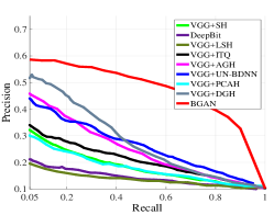
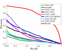
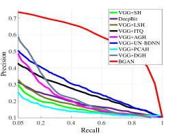
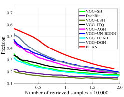
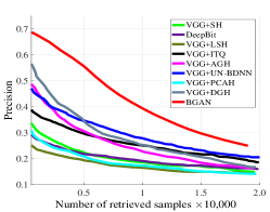
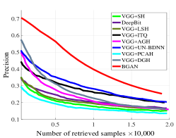
In this subsection, we compare our BGAN with different unsupervised hashing methods on three datasets. The results on mAP are shown in Table 3, and the precision is shown in Fig. 4. From Table 3 and Fig. 4, we have the following observations:
1) Our method significantly outperforms the other deep or non-deep hashing methods in all datasets. In CIFAR-10, the improvement of BGAN over the other methods is more significant, compared with that in NUS-WIDE and Flickr datasets. Specifically, it outperforms the best counterpart (Spherical+VGG) by 18.9%, 26.5%, 27.5% and 27.7% for 12, 24, 32 and 48-bit hash codes. One possible reason is that CIFAR-10 contains simple images, and the constructed neighborhood structure is more accurate than the other two datasets. BGAN improves the state-of-the-arts by 12.6%, 7.6%, 6.1% and 5.0% in NUS-WIDE dataset, and 11.4%, 14.3%, 12.0% and 13.1% in NUS-WIDE dataset.
2) Table 3 shows that Spherical+VGG is a strong competitor in terms of mAP, and Fig. 4 performs well for small number of retrieved samples (or recall). On the other hand, the performance of deep hashing methods (DeepBit (Lin et al., 2016) and DH (Erin Liong et al., 2015)) is not superior. A possible reason is the deep hashing methods use only 3 full connected layers to extract the features, which is not very powerful.
3) When we run the non-deep hashing methods on deep features, the performance is usually improved compared with the hand-crafted features. The performance gap is larger in CIFAR-10 and NUS-WIDE datasets than in Flickr dataset.
4) With the increase of code length, the performance of most hashing methods is improved accordingly. More specifically, the mAP improvements using deep features are generally more significant than that of non-deep features in CIFAR-10 dataset and NUS-WIDE dataset. An exception is SH, which has no improvement with the increase of code length.
We also compared with supervised hashing methods, and shown the mAP results on CIFAR-10 dataset in Table 6. It is obvious that our BGAN_s outperforms the state-of-the-art deep and non-deep supervised hashing algorithms by a large margin, which are 15.8%, 13.9%, 12.8% and 11.9% for 12, 24, 32, and 48-bits hash codes. This indicates that the performance improvement of BGAN is not only due to the constructed neighborhood structure, but also the other components.
4.5. The Study of Efficiency (RQ4)
In this subsection, we study the efficiency of our algorithm. First, we study the convergence of our BGAN in CIFAR-10 dataset, and the results on shown in Fig. 5. It can be seen that our method converges after a few epochs, which shows the efficiency of our solution.

We also report the training and testing time in CIFAR-10 dataset of our algorithm, and compare it with DH (Erin Liong et al., 2015) in Table 6. Since our BGAN has more parameters, it takes longer time for training and testing. However, BGAN is still very fast for generating the hash codes for a test image.
| Methods | Training time | Testing time |
|---|---|---|
| DH (Erin Liong et al., 2015) | 1 hour | 0.5 ms |
| BGAN | 5h | 3 ms |
4.6. Reconstruction Results
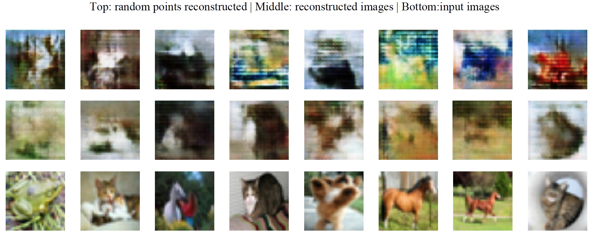
To evaluate the ability of image reconstruction using BGAN, we show some qualitative results on CIFAR-10 dataset in Fig. 6. The top row are the reconstructed results using random input, the second row are the reconstructed results from BGAN, and the last row are the original images. We can see that BGAN can reconstruct images which are similar to the original images.
5. Conclusion
In this work, we propose an unsupervised hashing which addresses two central problems remaining largely unsolved for image hashing: 1) how to directly generate binary codes without relaxation? 2) how to equip the binary representation with the ability of accurate image retrieval, beyond vivid image generation? First, we propose two equivalent but smoothed activation functions, and design a learning strategy whose solution converges to the results of sign activation. Second, we propose a loss function which consists of an adversarial loss, a content loss, and a neighborhood structure loss. Experimental results show that our BGAN doubled the performance of the state-of-the-arts in CIFAR-10 dataset, and also significantly outperformed the others on NUSWIDE, and Flickr datasets. In the future, it is necessary to improve the reconstruction accuracy of BGAN.
References
- (1)
- Allgower and Georg (2012) Eugene L Allgower and Kurt Georg. 2012. Numerical continuation methods: an introduction. Vol. 13. Springer Science & Business Media.
- Cao et al. (2017) Zhangjie Cao, Mingsheng Long, Jianmin Wang, and Philip S Yu. 2017. HashNet: Deep Learning to Hash by Continuation. arXiv preprint arXiv:1702.00758 (2017).
- Chen et al. (2016) Xi Chen, Yan Duan, Rein Houthooft, John Schulman, Ilya Sutskever, and Pieter Abbeel. 2016. InfoGAN: Interpretable Representation Learning by Information Maximizing Generative Adversarial Nets. (2016).
- Dai et al. (2016) Qi Dai, Jianguo Li, Jingdong Wang, and Yu-Gang Jiang. 2016. Binary Optimized Hashing. In ACM Multimedia. ACM, 1247–1256.
- Datar et al. (2004) Mayur Datar, Nicole Immorlica, Piotr Indyk, and Vahab S. Mirrokni. 2004. Locality-sensitive hashing scheme based on p-stable distributions. In Symposium on Computational Geometry.
- Do et al. (2016) Thanh-Toan Do, Anh-Dzung Doan, and Ngai-Man Cheung. 2016. Learning to hash with binary deep neural network. In ECCV. Springer, 219–234.
- Erin Liong et al. (2015) Venice Erin Liong, Jiwen Lu, Gang Wang, Pierre Moulin, and Jie Zhou. 2015. Deep hashing for compact binary codes learning. In Proceedings of the IEEE Conference on Computer Vision and Pattern Recognition. 2475–2483.
- Ge et al. (2014) Tiezheng Ge, Kaiming He, and Jian Sun. 2014. Graph Cuts for Supervised Binary Coding. In ECCV.
- Gong et al. (2013a) Y. Gong, S Lazebnik, A Gordo, and F Perronnin. 2013a. Iterative quantization: a Procrustean approach to learning binary codes for large-scale image retrieval.. In IEEE Conference on Computer Vision and Pattern Recognition. 817–824.
- Gong et al. (2013b) Yunchao Gong, Svetlana Lazebnik, Albert Gordo, and Florent Perronnin. 2013b. Iterative Quantization: A Procrustean Approach to Learning Binary Codes for Large-Scale Image Retrieval. IEEE Trans. PAMI 35, 12 (2013), 2916–2929.
- Goodfellow et al. (2014) Ian Goodfellow, Jean Pouget-Abadie, Mehdi Mirza, Bing Xu, David Warde-Farley, Sherjil Ozair, Aaron Courville, and Yoshua Bengio. 2014. Generative adversarial nets. In Advances in neural information processing systems. 2672–2680.
- Gu et al. (2016) Yun Gu, Chao Ma, and Jie Yang. 2016. Supervised Recurrent Hashing for Large Scale Video Retrieval. In Proceedings of the 2016 ACM on Multimedia Conference. ACM, 272–276.
- Guo et al. (2016) Jinma Guo, Shifeng Zhang, and Jianmin Li. 2016. Hash learning with convolutional neural networks for semantic based image retrieval. In Pacific-Asia Conference on Knowledge Discovery and Data Mining. Springer, 227–238.
- He et al. (2015) Kaiming He, Xiangyu Zhang, Shaoqing Ren, and Jian Sun. 2015. Deep Residual Learning for Image Recognition. arXiv preprint arXiv:1512.03385 (2015).
- Heo et al. (2015) Jae-Pil Heo, Youngwoon Lee, Junfeng He, Shih-Fu Chang, and Sung-Eui Yoon. 2015. Spherical Hashing: Binary Code Embedding with Hyperspheres. IEEE Trans. Pattern Anal. Mach. Intell. 37, 11 (2015), 2304–2316.
- Hu et al. (2014) Yao Hu, Zhongming Jin, Hongyi Ren, Deng Cai, and Xiaofei He. 2014. Iterative Multi-View Hashing for Cross Media Indexing. In ACM MM.
- Irie et al. (2014) Go Irie, Zhenguo Li, Xiao-Ming Wu, and Shih-Fu Chang. 2014. Locally Linear Hashing for Extracting Non-linear Manifolds. In CVPR.
- Jégou et al. (2011) Hervé Jégou, Matthijs Douze, and Cordelia Schmid. 2011. Product Quantization for Nearest Neighbor Search. IEEE Trans. PAMI 33, 1 (2011), 117–128.
- Jin et al. (2013) Zhongming Jin, Yao Hu, Yue Lin, Debing Zhang, Shiding Lin, Deng Cai, and Xuelong Li. 2013. Complementary Projection Hashing. In IEEE International Conference on Computer Vision, ICCV 2013, Sydney, Australia, December 1-8, 2013. 257–264.
- Kang et al. (2016) Wang-Cheng Kang, Wu-Jun Li, and Zhi-Hua Zhou. 2016. Column Sampling based Discrete Supervised Hashing. In AAAI.
- Kingma and Welling (2013) Diederik P Kingma and Max Welling. 2013. Auto-encoding variational bayes. arXiv preprint arXiv:1312.6114 (2013).
- Krizhevsky et al. (2012) Alex Krizhevsky, Ilya Sutskever, and Geoffrey E Hinton. 2012. Imagenet classification with deep convolutional neural networks. In Advances in neural information processing systems. 1097–1105.
- Lai et al. (2015) Hanjiang Lai, Yan Pan, Ye Liu, and Shuicheng Yan. 2015. Simultaneous feature learning and hash coding with deep neural networks. In CVPR. 3270–3278.
- Larsen et al. (2015) Anders Boesen Lindbo Larsen, Søren Kaae Sønderby, Hugo Larochelle, and Ole Winther. 2015. Autoencoding beyond pixels using a learned similarity metric. arXiv preprint arXiv:1512.09300 (2015).
- Ledig et al. (2016) Christian Ledig, Lucas Theis, Ferenc Huszar, Jose Caballero, Andrew P. Aitken, Alykhan Tejani, Johannes Totz, Zehan Wang, and Wenzhe Shi. 2016. Photo-Realistic Single Image Super-Resolution Using a Generative Adversarial Network. CoRR abs/1609.04802 (2016).
- Li et al. (2015) Wu Jun Li, Sheng Wang, and Wang Cheng Kang. 2015. Feature Learning based Deep Supervised Hashing with Pairwise Labels. Computer Science (2015).
- Lin et al. (2014) Guosheng Lin, Chunhua Shen, Qinfeng Shi, Anton van den Hengel, and David Suter. 2014. Fast Supervised Hashing with Decision Trees for High-Dimensional Data. In CVPR.
- Lin et al. (2016) Kevin Lin, Jiwen Lu, Chu-Song Chen, and Jie Zhou. 2016. Learning compact binary descriptors with unsupervised deep neural networks. In Proceedings of the IEEE Conference on Computer Vision and Pattern Recognition. 1183–1192.
- Liu et al. (2014b) Wei Liu, Cun Mu, Sanjiv Kumar, and Shih-Fu Chang. 2014b. Discrete Graph Hashing. In NIPS. 3419–3427.
- Liu et al. (2012) Wei Liu, Jun Wang, Rongrong Ji, Yu-Gang Jiang, and Shih-Fu Chang. 2012. Supervised hashing with kernels. In CVPR.
- Liu et al. (2011) Wei Liu, Jun Wang, Sanjiv Kumar, and Shih-Fu Chang. 2011. Hashing with Graphs. In ICML.
- Liu et al. (2014a) Xianglong Liu, Junfeng He, Cheng Deng, and Bo Lang. 2014a. Collaborative Hashing. In CVPR.
- Norouzi and Fleet (2011) Mohammad Norouzi and David J. Fleet. 2011. Minimal Loss Hashing for Compact Binary Codes. In ICML.
- Norouzi and Fleet (2013) Mohammad Norouzi and David J. Fleet. 2013. Cartesian K-Means. In CVPR.
- Radford et al. (2015) Alec Radford, Luke Metz, and Soumith Chintala. 2015. Unsupervised representation learning with deep convolutional generative adversarial networks. arXiv preprint arXiv:1511.06434 (2015).
- Reed et al. (2016) Scott Reed, Zeynep Akata, Xinchen Yan, Lajanugen Logeswaran, Bernt Schiele, and Honglak Lee. 2016. Generative Adversarial Text to Image Synthesis. (2016).
- Rongkai Xia and Yan (2014) Hanjiang Lai Cong Liu Rongkai Xia, Yan Pan and Shuicheng Yan. 2014. Supervised Hashing for Image Retrieval via Image Representation Learning. In AAAI. 2156–2162.
- Salakhutdinov and Hinton (2009) Ruslan Salakhutdinov and Geoffrey Hinton. 2009. Semantic hashing. International Journal of Approximate Reasoning 50, 7 (2009), 969–978.
- Shakhnarovich et al. (2008) Gregory Shakhnarovich, Trevor Darrell, and Piotr Indyk. 2008. Nearest-Neighbor Methods in Learning and Vision. IEEE Transactions on Neural Networks 19, 2 (2008), 377.
- Strecha et al. (2012) Christoph Strecha, Alexander M Bronstein, Michael M Bronstein, and Pascal Fua. 2012. LDAHash: Improved matching with smaller descriptors. IEEE Trans. Pattern Anal. Mach. Intell. 34, 1 (2012), 66–78.
- Szegedy et al. (2015) Christian Szegedy, Wei Liu, Yangqing Jia, Pierre Sermanet, Scott Reed, Dragomir Anguelov, Dumitru Erhan, Vincent Vanhoucke, and Andrew Rabinovich. 2015. Going deeper with convolutions. In Proceedings of the IEEE Conference on Computer Vision and Pattern Recognition. 1–9.
- Wang et al. (2012) Jun Wang, Sanjiv Kumar, and Shih-Fu Chang. 2012. Semi-Supervised Hashing for Large-Scale Search. IEEE Trans. PAMI 34, 12 (2012), 2393–2406.
- Wang et al. (2014a) Jingdong Wang, Heng Tao Shen, Jingkuan Song, and Jianqiu Ji. 2014a. Hashing for Similarity Search: A Survey. CoRR abs/1408.2927 (2014).
- Wang et al. (2013) Jianfeng Wang, Jingdong Wang, Nenghai Yu, and Shipeng Li. 2013. Order preserving hashing for approximate nearest neighbor search. In ACM MM.
- Wang et al. (2014b) Qifan Wang, Luo Si, and Dan Zhang. 2014b. Learning to Hash with Partial Tags: Exploring Correlation between Tags and Hashing Bits for Large Scale Image Retrieval. In ECCV.
- Weiss et al. (2008) Yair Weiss, Antonio Torralba, and Robert Fergus. 2008. Spectral Hashing. In NIPS.
- Yang et al. (2017) Huei-Fang Yang, Kevin Lin, and Chu-Song Chen. 2017. Supervised Learning of Semantics-Preserving Hash via Deep Convolutional Neural Networks. IEEE Transactions on Pattern Analysis and Machine Intelligence (2017).
- Zhang et al. (2014) Peichao Zhang, Wei Zhang, Wu-Jun Li, and Minyi Guo. 2014. Supervised Hashing with Latent Factor Models. In Proceedings of the 37th International ACM SIGIR Conference on Research & Development in Information Retrieval (SIGIR ’14). 173–182.
- Zhu et al. (2016) Han Zhu, Mingsheng Long, Jianmin Wang, and Yue Cao. 2016. Deep Hashing Network for Efficient Similarity Retrieval.. In AAAI. 2415–2421.