Finite temperature Green’s function approach for excited state and thermodynamic properties of cool to warm dense matter

Abstract

We present a finite-temperature extension of the retarded cumulant Green’s function for calculations of exited-state and thermodynamic properties of electronic systems. The method incorporates a cumulant to leading order in the screened Coulomb interaction $W$ and improves excited state properties compared to the $GW$ approximation of many-body perturbation theory. Results for the homogeneous electron gas are presented for a wide range of densities and temperatures, from cool to warm dense matter regime, which reveal several hitherto unexpected properties. For example, correlation effects remain strong at high $T$ while the exchange-correlation energy becomes small. In addition, the spectral function broadens and damping increases with temperature, blurring the usual quasi-particle picture. Similarly Compton scattering exhibits substantial many-body corrections that persist at normal densities and intermediate $T$. Results for exchange-correlation energies and potentials are in good agreement with existing theories and finite-temperature DFT functionals.

Finite temperature (FT) effects in electronic systems are both of fundamental interest and practical importance. These effects vary markedly depending on whether the temperature $T$ is larger or smaller than the Fermi temperature $T_{F}$ (typically a few eV). At “cool” temperatures, where $T$ is much smaller than $T_{F}$, electrons are nearly degenerate, and Fermi factors and excitations such as phonons dominate the thermal behavior Allen and Mitrović (1982); Allen and Heine (1976); Eiguren and Ambrosch-Draxl (2008). In contrast thermal occupations become nearly semi-classical and electronic excitations such as plasmons become important in the warm-dense-matter (WDM) regime, where $T$ is of order $T_{F}$ or larger, and condensed matter is partially ionized. Recently there has been considerable interest in both experimental and theoretical investigations of WDM for applications ranging from laser-shocked systems and inertial confinement fusion to astrophysics Koenig et al. (2005); Driver and Militzer (2016). Many of these studies focus on equilibrium thermodynamic properties, e.g., using the FT generalization of density functional theory (DFT) Dharma-wardana (2013); Sjostrom and Dufty (2013); Burke et al. (2016). Although in principle, FT DFT is exact Hohenberg and Kohn (1964); Kohn and Sham (1965); Mermin (1965), practical applications require exchange-correlation functionals which must be approximated, e.g., by constrained fits Karasiev et al. (2014) to theoretical electron gas calculations Brown et al. (2013); Spink et al. (2013); Burke et al. (2016); Tanaka and Ichimaru (1986); Singwi et al. (1968); Yan et al. (2000). However, these approaches have various limitations. First, many materials properties such as optical and x-ray spectra depend on quasi-particle or excited-state effects. For example, band-gaps depend on quasi-particle energies, and calculations of x-ray spectra Cho et al. (2011) and Compton scattering require correlation corrections Mattern et al. (2012). Although methods like quantum Monte-Carlo and the random phase approximation (RPA) can provide accurate correlation energies, they are not directly applicable to such excited state properties. Secondly, currently available exchange-correlation functionals can exhibit unphysical behavior outside the range of validity of theoretical data Karasiev et al. (2016). On the other hand Green’s function (GF) methods within many-body perturbation theory (MBPT) provide a systematic framework for calculations of both excited state and thermodynamic equilibrium properties, including total and correlation energies. Such methods are widely used at $T=0$, as are FT generalizations in applications ranging from phonon-effects at low $T$ Engelsberg and Schrieffer (1963); Allen and Mitrović (1982); Eiguren and Ambrosch-Draxl (2008); Allen and Heine (1976) to nuclear matter Rios et al. (2008). Nevertheless, while the theoretical formalism is well established, relatively little attention has been devoted to practical applications of FT GF methods at high $T$. Methods for FT exchange-correlation potentials have also been developed Dharma-wardana and Taylor (1981), and quasi-particle corrections have been addressed using the quasiparticle self-consistent $GW$ approximation (QPSCGW) Faleev et al. (2006), but many excited state properties remain unexplored.

In an effort to address these limitations, we have developed a finite-$T$ extension of the retarded cumulant Green’s function Hedin (1999); Kas et al. (2014). The cumulant approach has been successful at zero $T$ in elucidating correlation effects beyond the $GW$ approximation of MBPT in a variety of contexts Kas et al. (2015, 2016); Lischner et al. (2014); Caruso et al. (2015); Caruso and Giustino (2015); Story et al. (2014). For example, in contrast to $GW$, the approach explains the multiple-plasmon satellites observed in x-ray photoemission spectra (XPS) Guzzo et al. (2011); Aryasetiawan et al. (1996); Kas et al. (2015); Lee et al. (2012); Zhou et al. (2015). However, the behavior in WDM is hitherto unexplored and exhibits a number of unusual and unexpected properties. As an application relevant to FT DFT, we have implemented the approach for the homogeneous electron gas (HEG). Our results show that besides reductions in quasi-particle energy shifts (and hence band-gaps) with increasing $T$, the spectral function broadens and the excited states become strongly damped, corresponding to short mean-free-paths, blurring of the conventional quasi-particle picture, and smeared-out band-structure. Finally thermodynamic properties including exchange-correlation energies are calculated using the Galitskii-Migdal-Koltun (GMK) sum rule Martin and Schwinger (1959); Mahan (2000); Koltun (1974), which serves as a quantitative check on our approximations and yields results that compare well with existing theories Brown et al. (2013), and with FT DFT functionals Karasiev et al. (2014).

Briefly our approach is based on the finite-$T$ retarded Green’s function formalism Mahan (2000). Below we outline the key elements of the approach. The retarded one-particle FT Green’s function $G(\omega)$ satisfies a Dyson equation $G=G^{0}+G^{0}\Sigma G$ Dash et al. (2010), where $\Sigma$ is the retarded self-energy. Formally $\Sigma$ can be found by analytical continuation of the Matsubara self-energy to real frequencies, and can be expressed in terms of $G$, the screened Coulomb interaction $W=\epsilon^{-1}v$, and a vertex function $\Gamma$ Hedin (1999); Dash et al. (2010). Here and below matrix indices are suppressed unless otherwise specified, and we use atomic units $e=\hbar=m=1$. Most practical calculations currently ignore vertex corrections ($\Gamma=1$). With this restriction, a variety of FT approximations have been used: For example, the $GW$ approximation is based on the Dyson equation and MBPT to first order in $W$; then $\Gamma=1$ and $G=G^{0}+G^{0}\Sigma^{GW}G$ Hedin (1999); Hybertsen and Louie (1985). As a further approximation, the quasi-particle self-consistent $GW$ approach (QPSCGW) Faleev et al. (2006) starts with the GF on the Keldysh contour; while self-consistency is carried out, vertex corrections, satellites, and damping are ignored. In contrast the retarded cumulant GF method used here is based on an exponential representation (see below) that builds in implicit dynamic vertex corrections Hedin (1999); Guzzo et al. (2011). This form can be justified using the quasi-boson approximation Hedin (1999), in which electron-electron interactions are represented in terms of electrons coupled to bosonic excitations. This approach is an improvement over $GW$ for spectral properties Zhou et al. (2015), and is exact for certain models Langreth (1970). More elaborate GF methods exist at least in principle, including higher order MBPT Gunnarsson et al. (1994); Pavlyukh et al. (2013), and dynamical mean-field theory with impurity Green’s function’s Deng et al. (2013); Casula et al. (2012), but are more demanding computationally.

The retarded cumulant expansion begins with an exponential ansatz for the FT GF in the time-domain for a given single-particle state $k$ in which $G$ is assumed to be diagonal, and the spectral function $A_{k}(\omega)$ is obtained from its Fourier transform,

$$G_{k}(t) = -i\theta(t)e^{-i\varepsilon^{x}_{k}t}e^{{\tilde{C}}_{k}(t)},$$ (1)

$$A_{k}(\omega) = -\frac{1}{\pi}{\rm Im}\,\int d\omega e^{i\omega t}G_{k}(t).$$ (2)

In this formulation static exchange and correlation contributions are separated $C_{k}(t)=-i\Sigma_{k}^{x}t+\tilde{C}_{k}(t)$, and all correlation effects are included in the dynamic part $\tilde{C}_{k}(t)$ of the cumulant. Here $\Sigma^{x}_{k}=\Sigma_{\bf q}n_{\bf k-q}v_{\bf q}$ is the exchange part of the FT Hartree-Fock one-particle energy, $\varepsilon_{k}^{x}=\varepsilon_{k}+\Sigma_{k}^{x}$, $\varepsilon_{k}=k^{2}/2$ is the bare energy, and $v_{\bf q}=4\pi/q^{2}$ is the bare Coulomb interaction. This formulation is directly analogous to that for $T=0$ Kas et al. (2014), apart from implicit temperature dependence in it’s ingredients. The retarded cumulant $C_{k}(t)$ can be obtained by matching terms in powers of $W$ to those of the Dyson equation Kas et al. (2014); Zhou et al. (2015). Carried to all orders the cumulant GF is formally exact; however, by limiting the theory to first order in $W$, $G^{0}C=G^{0}\Sigma^{GW}G^{0}$, the retarded GW self energy $\Sigma^{GW}$ is sufficient to define the FT cumulant. $\tilde{C}(t)$ has a Landau representation, which implies a positive-definite spectral function and conserves spectral weight Landau (1944); Langreth (1970); Hedin (1999),

$${\tilde{C}}_{k}(t) = \int d\omega\frac{\gamma_{k}(\omega)}{\omega^{2}}(e^{-i\omega t}+i\omega t-1),$$ (3)

$$\gamma_{k}(\omega) = \frac{1}{\pi}\left|{\rm Im}\,\Sigma_{k}(\omega+\varepsilon_{k})\right|.$$ (4)

The kernel $\gamma_{k}(\omega)$ reflects the quasi-boson excitation spectrum in the system, with peaks corresponding to those in $W(\omega)\propto{\rm Im}\Sigma_{k}(\omega+\varepsilon_{k})$.

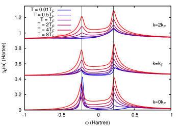
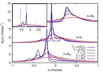
Figure 1: (Color online) FT retarded cumulant kernel $\gamma_{k}(T,\omega)$ (top); and spectral function $A_{k}(T,\omega)$ for the HEG (bottom) for $r_{s}=4$. Vertical lines in the top plot are shown at $\pm\omega_{p}$. Note the enhanced symmetry of both $\gamma_{k}$ and $A_{k}$ at high-$T$. The inset shows a comparison of the cumulant (solid) and GW (dashes) spectral functions at $k=0$ for the lowest and highest temperatures.

The basic ingredients in the theory Eq. (1-3), are thus $G^{0}$, the $GW$ self-energy $\Sigma^{GW}$, and the screened Coulomb interaction $W(q,\omega)=\epsilon^{-1}(q,\omega)v_{q}$, where $\epsilon(q,\omega)$ is the dielectric function. These quantities can be calculated using standard finite-$T$ MBPT Allen and Mitrović (1982); Mahan (2000), starting from the Matsubara Green’s function. The finite-$T$ analog of the $GW$ self energy for electrons coupled to bosons is (cf. the Migdal approximation Allen and Mitrović (1982)),

$$\Sigma^{GW}(\omega,T)=\int d\omega^{\prime}\frac{d^{3}q}{(2\pi)^{3}}|{\rm Im}\,W(q,\omega^{\prime})|\times$$

$$\times\left[\frac{f(\varepsilon_{k-q})+N(\omega^{\prime})}{\omega+\omega^{\prime}-\varepsilon_{k-q}+i\delta}+\frac{1-f(\varepsilon_{k-q})+N(\omega^{\prime})}{\omega-\omega^{\prime}-\varepsilon_{k-q}+i\delta}\right].$$ (5)

Here $N(\omega)=1/(e^{\beta\omega}-1)$ is the Bose factor, $f(\varepsilon)=1/(e^{\beta(\varepsilon-\mu)}+1)$ the Fermi factor, $\beta=1/k_{B}T$, and $\mu(T)$ is the chemical potential, as determined below. The imaginary part of $\Sigma^{GW}(\omega)$ yields $\gamma_{k}(\omega)$ (Fig. 1 top). At high-$T$ the behavior of $\gamma_{k}$ is dominated by the Bose factors $N(\omega)\sim k_{B}T/\omega$ and becomes strongly symmetric about $\omega=0$. To obtain $W$ we use the FT-RPA approximation for the dielectric function,

$$\epsilon(q,\omega)=1+2v_{q}\int\frac{d^{3}k}{(2\pi)^{3}}\frac{f_{k+q}-f_{k}}{\omega-\varepsilon_{k+q}+\varepsilon_{k}}.$$ (6)

The imaginary part of $\epsilon(q,\omega)$ is analytic Khanna and Glyde (1976); Arista and Brandt (1984), and the real part is calculated via Kramers-Kronig transform. This yields the finite-$T$ loss function $L(q,\omega)=|{\rm Im}\,\epsilon^{-1}(q,\omega)|$. For the HEG $L(q>0,\omega)$ exhibits broadened and blue-shifted plasmon-peaks with increasing $T$ Arista and Brandt (1984). The chemical potential $\mu=\mu(T,N)$ implicit in the Fermi factors $f(\omega)$ is determined by enforcing charge conservation $\Sigma_{\bf k}\,n_{k}=\langle N(T)\rangle$, where the single-particle occupation numbers $n_{k}(T)$ are given by a trace over the spectral function Martin and Schwinger (1959),

$$n_{k}(\mu,T)=\int_{-\infty}^{\infty}d\omega\,A_{k}(\omega)f(\omega),$$ (7)

Occupation numbers can be measured e.g., by Compton scattering Mattern et al. (2012); Klevak et al. (2014); Huotari et al. (2010), and are sensitive to the many-body correlation effects in $A_{k}$.

Note that at low-$T$, $A_{k}(\omega)$ exhibits multiple-satellites for $k<k_{F}$ while for $k>k_{F}$ and at $T>T_{F}$, the quasi-particle peak broadens, and overlaps the satellites. Thus in WDM the structure of $A_{k}$ blurs into single asymmetric peak with a centroid at $\varepsilon_{k}^{x}(T)$ and root mean square width $\delta_{k}$ given by the 2nd cumulant moment of $A_{k}(\omega)$ $\delta_{k}^{2}=\tilde{C}_{k}^{\prime\prime}(0)=\int d\omega\,\gamma_{k}(\omega)$. A dimensionless measure of correlation is given by the satellite strength in the spectral function $a_{k}\equiv\ln(1/Z_{k})=\int d\omega\gamma_{k}(\omega)/\omega^{2}$, where $Z_{k}$ is the renormalization constant, which is determined from the last term in Eq. (3). This measure corresponds to the mean number of bosonic excitations and is of order $0.2r_{s}^{3/4}$ ($r_{s}$ being the Wigner-Seitz radius) for plasmons at $T=0$ Hedin (1999). Surprisingly $a_{k}$ is only weakly dependent on temperature with $Z_{k_{F}}\approx 0.6$ at $r_{s}=4$. Formally the structure of the Landau cumulant in Eq. (3) is consistent with the conventional quasi-particle picture, i.e., a renormalized main peak red-shifted by a “relaxation energy” $\Delta_{k}$ and a series of satellites. The correlation part of the quasi-particle energy shift $\Delta_{k}$ is obtained from middle term in Eq. (3), while the first term gives rise to satellites at multiples of the plasmon peak $\omega_{p}$. The quasi-particle energy is then $\varepsilon^{qp}_{k}=\varepsilon_{k}+\Delta_{k}$,

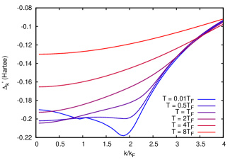
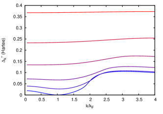
Figure 2: (Color online) Real (top) and imaginary (bottom) parts of the quasiparticle correction $\Delta_{k}$ shown for varying temperature.

where

$$\Delta_{k}=\Sigma_{k}^{x}+\int d\omega\,\frac{\gamma_{k}(\omega)}{(\omega-i\delta)}.$$ (8)

The real part $\Delta_{k}^{\prime}$ is the relaxation energy which is comparable to that in QPSCGW Faleev et al. (2006). Due to the increasingly symmetrical behavior of $\gamma_{k}(\omega)$, $\Delta^{\prime}$ decreases smoothly with $T$. However, a striking difference with the $T=0$ behavior is the presence of an imaginary part $\Delta_{k}^{\prime\prime}$ even at the Fermi momentum, which becomes large at high-$T$ since $\gamma_{k}(0)\neq 0$. This behavior implies strongly damped propagators that blur the usual quasi-particle picture, smearing band-gaps and band-structures. This behavior is clearly evident in the spectral function $A_{k}(\omega)=(1/\pi)|{\rm Im}\,G_{k}(\omega)|$ Mahan (2000); Martin and Schwinger (1959), which is directly related to x-ray photoemission spectra (XPS) (Fig. 1). In contrast, the GW spectral function retains satellite structure even at high $T$ (Fig. 1 inset).

One of the advantages of the cumulant formalism is that is provides an alternative approach to calculate thermodynamic equilibrium properties. Remarkably, knowledge of $\mu(T)$ is sufficient to determine the FT DFT exchange-correlation potential for the HEG Perrot et al. (2000), $v_{xc}(T)\equiv\mu_{xc}(T)=\mu(T)-\mu_{0}(T)$, where $\mu_{0}(T)$ is the chemical potential for non-interacting electrons (Fig. 3).

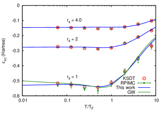
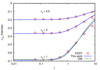
Figure 3: (Color online) Finite-$T$ exchange-correlation energy per particle (top) and potential $v_{xc}$ vs $\tau=T/T_{F}$ for the HEG from the cumulant expansion (blue), compared to RPIMC (crosses) and constrained fits (red circles). The inset shows the quasiparticle renormalization factor at the Fermi momentum $Z_{k_{F}}$ as a function of $T$.

Clearly the agreement with existing FT DFT exchange-correlation potentials and theoretical calculations is quite good. Moreover, the FT total energy per particle $\varepsilon(T)\equiv E(T)/N$, can be calculated from the GMK sum-rule Martin and Schwinger (1959); Mahan (2000); Koltun (1974),

$$\varepsilon(T) =\sum_{k}\int d\omega\,\left[\omega+\varepsilon_{k}\right]A_{k}(\omega)f(\omega),$$

$$=\varepsilon_{H}+\varepsilon_{xc},$$ (9)

which is valid for any Hamiltonian with only pair interactions. Here $\varepsilon_{H}$ is the Hartree energy. This relation is similar in form to the zero-$T$ Galitskii-Migdal sum-rule, except for the Fermi factor. Our results for $\varepsilon_{xc}(T)$ for the HEG are shown in Fig. 3.

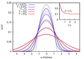
Figure 4: (Color online) Finite-$T$ Compton spectrum compared to the free-electron $T=0$ result at $r_{s}=4$ and ${q}=3$ Bohr^-1. The inset shows the difference between the effective temperature $T^{*}$ at which the free-electron calculation matches the cumulant result at $T$.

Clearly the agreement between the cumulant results, accurate restricted path-integral Monte Carlo (RPIMC) calculations Brown et al. (2013), and existing FT DFT functionals Karasiev et al. (2014) is quite good. At $T=0$, $\varepsilon_{xc}$ was found to be slightly better with the retarded cumulant than with $G_{0}W_{0}$, but self-consistent $GW$ gave better total energies Kas et al. (2014). Finally, we calculate the Compton spectrum (Fig. 4) following Ref. Schülke et al. (1996),

$$J_{q}(\omega)=\sum_{\bf q}\int d\omega A_{\bf k}(\omega)A_{\bf k+q}(\omega+\omega^{\prime})f(\omega)f(\omega+\omega^{\prime}).$$ (10)

At small $T$, effects of correlation are very noticeable, leading to an effective temperature $T^{*}$ (i.e. the temperature at which free-electron calculations match the interacting one) of $(T^{*}-T)/T_{F}\approx 0.3$ (see inset), while at high-$T$ the effect is smaller but non-negligible, $(T^{*}-T)/T_{F}\approx 0.1$.

In summary we have developed a finite-$T$ Green’s function approach for calculations of both excited state and thermodynamic properties over a wide range of densities and temperatures. Our approach is based on the retarded cumulant expansion to first order in $W$. This approximation greatly simplifies the theory and provides a practical approach both for calculations and the interpretation of exchange and correlation effects in terms of the behavior of retarded cumulant $C_{k}(t)$, which is directly related to the FT GW self energy $\Sigma^{GW}$. The cumulant GF builds in an approximate dynamic vertex, going beyond the $GW$ approximation, yet is no more difficult to calculate. Differences with respect to GW provide a measure of vertex effects and hence the accuracy of the theory. Although we have focused on the HEG, reflecting the importance of density fluctuations at high-$T$, the cumulant can be generalized to include additional quasi-boson excitations such as phonons since the leading cumulant is linear in bosonic couplings Story et al. (2014). The method provides an attractive complement to FT DFT, RPA, and RPIMC methods which are appropriate for correlation energies but inapplicable for many excited state properties. Illustrative results for the HEG explain the crossover in behavior from cool to WDM regimes and the blurring of the conventional quasi-particle picture. The crossover is largely due to an enhanced coupling to density fluctuations at high-$T$. We find that correlation effects remain strong at all temperatures and can have significant effects on spectral properties. Calculations of thermodynamic equilibrium quantities including exchange-correlation energies and potentials are in good agreement - typically within a few percent - with existing DFT functionals and quantum Monte Carlo (QMC) calculations. Many extensions are possible, ranging from excited state, spectroscopic to thermodynamic properties of realistic systems, and potentially to the development of improved FT DFT functionals Burke et al. (2016) e.g., in regimes inaccessible to conventional methods.

Acknowledgments: We thank K. Burke, G. Bertsch, V. Karasiev, L. Reining, E. Shirley, G. Seidler, T. Devereaux, and S. Trickey for comments and suggestions. This work is supported by DOE BES Grant DE-FG02-97ER45623.

References

- Allen and Mitrović (1982) P. B. Allen and B. Mitrović, in Solid State Physics, edited by H. Ehrenreich, F. Seitz, and D. Turnbull (Academic Press, 1982), vol. 37, pp. 1–92.
- Allen and Heine (1976) P. Allen and V. Heine, J. Phys. C 9, 2305 (1976).
- Eiguren and Ambrosch-Draxl (2008) A. Eiguren and C. Ambrosch-Draxl, Phys. Rev. Lett. 101, 036402 (2008).
- Koenig et al. (2005) M. Koenig, A. Benuzzi-Mounaix, A. Ravasio, T. Vinci, N. Ozaki, S. Lepape, D. Batani, G. Huser, T. Hall, D. Hicks, et al., Plasma Phys. Control. Fusion 47, B441 (2005).
- Driver and Militzer (2016) K. P. Driver and B. Militzer, Phys. Rev. B 93, 064101 (2016).
- Dharma-wardana (2013) M. W. C. Dharma-wardana, J. Phys.: Conf. Ser. 442, 012030 (2013).
- Sjostrom and Dufty (2013) T. Sjostrom and J. Dufty, Phys. Rev. B 88, 115123 (2013).
- Burke et al. (2016) K. Burke, J. C. Smith, P. E. Grabowski, and A. Pribram-Jones, Phys. Rev. B 93, 195132 (2016).
- Hohenberg and Kohn (1964) P. Hohenberg and W. Kohn, Phys. Rev. 136, B864 (1964).
- Kohn and Sham (1965) W. Kohn and L. J. Sham, Phys. Rev. 140, A1133 (1965).
- Mermin (1965) N. D. Mermin, Phys. Rev. 137, A1441 (1965).
- Karasiev et al. (2014) V. V. Karasiev, T. Sjostrom, J. Dufty, and S. B. Trickey, Phys. Rev. Lett. 112, 076403 (2014).
- Brown et al. (2013) E. W. Brown, B. K. Clark, J. L. DuBois, and D. M. Ceperley, Phys. Rev. Lett. 110, 146405 (2013).
- Spink et al. (2013) G. G. Spink, R. J. Needs, and N. D. Drummond, Phys. Rev. B 88, 085121 (2013).
- Tanaka and Ichimaru (1986) S. Tanaka and S. Ichimaru, J. Phys. Soc. Jpn. 55, 2278 (1986).
- Singwi et al. (1968) K. S. Singwi, M. P. Tosi, R. H. Land, and A. Sjölander, Phys. Rev. 176, 589 (1968).
- Yan et al. (2000) Z. Yan, J. P. Perdew, and S. Kurth, Phys. Rev. B 61, 16430 (2000).
- Cho et al. (2011) B. I. Cho, K. Engelhorn, A. A. Correa, T. Ogitsu, C. P. Weber, H. J. Lee, J. Feng, P. A. Ni, Y. Ping, A. J. Nelson, et al., Phys. Rev. Lett. 106, 167601 (2011).
- Mattern et al. (2012) B. A. Mattern, G. T. Seidler, J. J. Kas, J. I. Pacold, and J. J. Rehr, Phys. Rev. B 85, 115135 (2012).
- Karasiev et al. (2016) V. V. Karasiev, L. Calderín, and S. B. Trickey, Phys. Rev. E 93, 063207 (2016).
- Engelsberg and Schrieffer (1963) S. Engelsberg and J. R. Schrieffer, Phys. Rev. 131, 993 (1963).
- Rios et al. (2008) A. Rios, A. Polls, A. Ramos, and H. Müther, Phys. Rev. C 78, 044314 (2008).
- Dharma-wardana and Taylor (1981) M. Dharma-wardana and R. Taylor, J. Phys. C: Solid State Phys. 14, 629 (1981).
- Faleev et al. (2006) S. V. Faleev, M. van Schilfgaarde, T. Kotani, F. Léonard, and M. P. Desjarlais, Phys. Rev. B 74, 033101 (2006).
- Hedin (1999) L. Hedin, J. Phys.: Condens. Matter 11, R489 (1999).
- Kas et al. (2014) J. J. Kas, J. J. Rehr, and L. Reining, Phys. Rev. B 90, 085112 (2014).
- Kas et al. (2015) J. J. Kas, F. D. Vila, J. J. Rehr, and S. A. Chambers, Phys. Rev. B 91, 121112(R) (2015).
- Kas et al. (2016) J. J. Kas, J. J. Rehr, and J. B. Curtis, Phys. Rev. B 94, 035156 (2016).
- Lischner et al. (2014) J. Lischner, D. Vigil-Fowler, and S. G. Louie, Phys. Rev. B 89, 125430 (2014).
- Caruso et al. (2015) F. Caruso, H. Lambert, and F. Giustino, Phys. Rev. Lett. 114, 146404 (2015).
- Caruso and Giustino (2015) F. Caruso and F. Giustino, Phys. Rev. B 92, 045123 (2015).
- Story et al. (2014) S. M. Story, J. J. Kas, F. D. Vila, M. J. Verstraete, and J. J. Rehr, Phys. Rev. B 90, 195135 (2014).
- Guzzo et al. (2011) M. Guzzo, G. Lani, F. Sottile, P. Romaniello, M. Gatti, J. J. Kas, J. J. Rehr, M. G. Silly, F. Sirotti, and L. Reining, Phys. Rev. Lett. 107, 166401 (2011).
- Aryasetiawan et al. (1996) F. Aryasetiawan, L. Hedin, and K. Karlsson, Phys. Rev. Lett. 77, 2268 (1996).
- Lee et al. (2012) A. J. Lee, F. D. Vila, and J. J. Rehr, Phys. Rev. B 86, 115107 (2012).
- Zhou et al. (2015) J. Zhou, J. Kas, L. Sponza, I. Reshetnyak, M. Guzzo, C. Giorgetti, M. Gatti, F. Sottile, J. Rehr, and L. Reining, J. Chem. Phys. 143 (2015).
- Martin and Schwinger (1959) P. C. Martin and J. Schwinger, Phys. Rev. 115, 1342 (1959).
- Mahan (2000) G. Mahan, Many-Particle Physics (Springer, 2000).
- Koltun (1974) D. S. Koltun, Phys. Rev. C 9, 484 (1974).
- Dash et al. (2010) L. Dash, H. Ness, and R. Godby, J. Chem. Phys. 132, 104113 (2010).
- Hybertsen and Louie (1985) M. S. Hybertsen and S. G. Louie, Phys. Rev. Lett. 55, 1418 (1985).
- Langreth (1970) D. C. Langreth, Phys. Rev. B 1, 471 (1970).
- Gunnarsson et al. (1994) O. Gunnarsson, V. Meden, and K. Schönhammer, Phys. Rev. B 50, 10462 (1994).
- Pavlyukh et al. (2013) Y. Pavlyukh, J. Berakdar, and A. Rubio, Phys. Rev. B 87, 125101 (2013).
- Deng et al. (2013) X. Deng, J. Mravlje, R. Žitko, M. Ferrero, G. Kotliar, and A. Georges, Phys. Rev. Lett. 110, 086401 (2013).
- Casula et al. (2012) M. Casula, A. Rubtsov, and S. Biermann, Phys. Rev. B 85, 035115 (2012).
- Landau (1944) L. Landau, J. Phys. USSR 8, 201 (1944).
- Khanna and Glyde (1976) F. C. Khanna and H. R. Glyde, Can. J. Phys. 54, 648 (1976).
- Arista and Brandt (1984) N. R. Arista and W. Brandt, Phys. Rev. A 29, 1471 (1984).
- Klevak et al. (2014) E. Klevak, J. J. Kas, and J. J. Rehr, Phys. Rev. B 89, 085123 (2014).
- Huotari et al. (2010) S. Huotari, J. A. Soininen, T. Pylkkänen, K. Hämäläinen, A. Issolah, A. Titov, J. McMinis, J. Kim, K. Esler, D. M. Ceperley, et al., Phys. Rev. Lett. 105, 086403 (2010).
- Perrot et al. (2000) F. Perrot, , and M. W. C. Dharma-wardana, Phys. Rev. B 62, 16536 (2000).
- Schülke et al. (1996) W. Schülke, G. Stutz, F. Wohlert, and A. Kaprolat, Phys. Rev. B 54, 14381 (1996).