Robustness of the semimetal state of Na₃Bi and Cd₃As₂ against Coulomb interaction

Abstract

We study the excitonic semimetal-insulator quantum phase transition in three-dimensional Dirac semimetal in which the fermion dispersion is strongly anisotropic. After solving the Dyson-Schwinger equation for the excitonic gap, we obtain a global phase diagram in the plane spanned by the parameter for Coulomb interaction strength and the parameter for fermion velocity anisotropy. We find that excitonic gap generation is promoted as the interaction becomes stronger, but is suppressed if the anisotropy increases. Applying our results to two realistic three-dimensional Dirac semimetals Na₃Bi and Cd₃As₂, we establish that their exact zero-temperature ground state is gapless semimetal, rather than excitonic insulator. Moreover, these two materials are far from the excitonic quantum critical point, thus there should not be any observable evidence for excitonic insulating behavior. This conclusion is in general agreement with the existing experiments of Na₃Bi and Cd₃As₂.

I INTRODUCTION

There has been increasing research interests in the physical properties of three-dimensional Dirac semimetal (3D DSM) that contains massless Dirac fermions at low energies Vafek14 ; Wehling14 ; Armitage17 . Such DSM state could emerge at the quantum critical point (QCP) between normal insulator and 3D topological insulator. Interestingly, 3D DSM has been observed in TiBiSe_2-xS_x XuSuYang11 ; Sato11 and Bi_2-xIn_xSe₃ Brahlek12 ; Wu13 by fine tuning the doping level. Theoretical studies WangZhiJun12 ; Wangzhijun13 predicted that a crystal-symmetry protected stable 3D DSM might be realized in such materials as A₃Bi (A=Na, K, Rb) and Cd₃As₂. Recent angle-resolved photoemission spectroscopy (ARPES) and quantum transport measurements reported evidences for the existence of 3D DSM state in Na₃Bi and Cd₃As₂ LiuZK14A ; Neupane14 ; LiuZK14B ; Borisenko14 ; HeLP14 .

Similar to 2D DSM Vafek14 ; Wehling14 ; CastoNeto09 ; Kotov12 and other semimetals Armitage17 ; Yan17 ; Hasan17 ; XuFang11 ; Fang12 ; YangNogasa14 , 3D DSM contains a number of discrete band-touching points, which means that the density of states (DOS) vanishes at the Fermi level. As a result, the Coulomb interaction between massless fermions is poorly screened and remains long-ranged Goswami11 ; Hosur12 ; Hofmann15 ; Throckmorton15 ; Sekine14 ; Gonzalez14 ; Gonzalez15 ; Braguta16 ; Braguta17 . Extensive theoretical studies on 2D DSM, with graphene being a prominent example, have revealed that a sufficiently strong long-range Coulomb interaction can induce excitonic-type pairing and as such opens a dynamical gap at the Fermi level Kotov12 ; CastroNetoPhysics09 ; Khveshchenko01 ; Gorbar02 ; Khveshchenko04 ; Liu09 ; Khveshchenko09 ; Gamayun10 ; Sabio10 ; Liu11 ; WangLiu11A ; WangLiu11B ; WangLiu12 ; Popovici13 ; WangLiu14 ; Carrington16 ; Xue17 ; Sharma17 ; Xiao17 ; Gamayun09 ; WangJianhui11 ; Katanin16 ; Vafek08 ; Gonzalez10 ; Gonzalez12 ; Drut09A ; Drut09B ; Drut09C ; Armour10 ; Armour11 ; Buividovich12 ; Ulybyshev13 ; Smith14 ; Tupitsyn17 ; Juan12 ; Kotikov16 . The particle-hole condensate breaks the chiral symmetry of the system Khveshchenko01 ; Gorbar02 , which is a condensed-matter realization of the non-perturbative phenomenon of dynamical chiral symmetry breaking that plays an essential role in hadron physics Roberts94 . Once a finite dynamical gap is generated, the semimetal state becomes unstable and the system is converted into an insulator Kotov12 ; CastroNetoPhysics09 . A nature question is whether a similar excitonic insulating transition also occurs in a 3D DSM.

The possible semimetal-insulator transition in 3D DSM has been studied by several groups Sekine14 ; Gonzalez14 ; Gonzalez15 ; Braguta16 ; Braguta17 . In Na₃Bi and Cd₃As₂, the $z$-component of the fermion velocity is considerably smaller than the other two components within the $x$-$y$ plane LiuZK14A ; Neupane14 ; LiuZK14B . Additionally, the magnitude of fermion velocity in these two materials is quite small. This implies that the Coulomb interaction may play a significant role at low energies. After performing Monte Carlo simulations, Braguta et al. Braguta16 ; Braguta17 claimed that both Na₃Bi and Cd₃As₂ lie deep in the excitonic insulating phase. This conclusion is somewhat surprising, because experiments did not find any evidence for the insulating behavior in these two materials LiuZK14A ; Neupane14 ; LiuZK14B ; Borisenko14 . It is necessary to examine whether the gapless semimetal state is robust against the long-range Coulomb interaction in Na₃Bi, Cd₃As₂, and other candidate 3D DSM materials.

In order to determine the true ground state of 3D DSM, we need to calculate the critical value of the Coulomb interaction strength that separates the semimetallic and insulating phases. For Na₃Bi and Cd₃As₂, the energy dispersion of 3D Dirac fermions can be written as

$$E=\pm\sqrt{v_{\parallel}^{2}k_{\parallel}^{2}+v_{z}^{2}k_{z}^{2}},$$ (1)

where $k_{\parallel}^{2}=k_{x}^{2}+k_{y}^{2}$. Here, $v_{\parallel}$ is the component of fermion velocity within the basal $x$-$y$ plane, and $v_{z}$ is the component along the $z$-direction. The effective strength of the Coulomb interaction is represented by the parameter Kotov12

$$\alpha = \frac{e^{2}}{v_{\parallel}\epsilon_{0}\epsilon_{r}},$$ (2)

where $e$ is the electron charge, $\epsilon_{0}$ the vacuum dielectric constant, and $\epsilon_{r}$ the relative dielectric constant. The value of $\epsilon_{r}$ is strongly material dependent. It is known Gorbar02 ; Khveshchenko04 ; Liu09 ; Khveshchenko09 ; Gamayun10 ; WangLiu12 ; Drut09A ; Drut09B ; Drut09C that an excitonic gap is generated only when $\alpha$ is larger than certain critical value $\alpha_{c}$. If $\alpha>\alpha_{c}$, the system has an insulating ground state, which can be detected by probing the transport properties at ultra low temperatures Geim11 ; Geim12 . If $\alpha$ is slightly smaller than $\alpha_{c}$, the exact zero-temperature ground state is semimetal. However, since the system is close to the excitonic insulating QCP, the quantum fluctuation of excitonic order parameter could be important at small distances, which may still have observable effects Hirata17 . If $\alpha\ll\alpha_{c}$, the system is deep in the semimetal phase, and does not exhibit any observable effects of insulating behavior.

In this paper, we calculate the value of $\alpha_{c}$ in 3D DSM by using the non-perturbative Dyson-Schwinger (DS) equation method Khveshchenko01 ; Gorbar02 ; Khveshchenko04 ; Liu09 ; Khveshchenko09 ; Gamayun10 ; Sabio10 ; Liu11 ; WangLiu11A ; WangLiu11B ; WangLiu12 ; Popovici13 ; WangLiu14 ; Carrington16 ; Sharma17 ; Xiao17 ; Appelquist88 ; Maris04 ; Feng06 ; Feng12A ; Feng12B ; LiJianFeng13 ; Janssen16 ; WangLiuZhang17 ; Gusynin16 ; Fischer18 . In some 3D DSMs, such as Na₃Bi and Cd₃As₂, the fermion dispersion is strongly anisotropic, and the $z$-component of fermion velocity is much smaller than that of the $x$-$y$ plane, namely $v_{z}\ll v_{\parallel}$. We need to define a velocity ratio and study how the ratio affects $\alpha_{c}$. A commonly used definition Braguta16 ; Braguta17 ; Sekine14 is

$$\eta=\frac{v_{z}}{v_{\parallel}}.$$ (3)

After solving the DS gap equation numerically, we obtain a global phase diagram of 3D DSM in the parameter space spanned by $\alpha$ and $\eta$. It is found that $\alpha_{c}$ exhibits a non-monotonic dependence on the velocity anisotropy, analogous to what happens in 2D DSM Xiao17 . We demonstrate that such non-monotonic dependence results from the improper definitions of $\alpha$ and $\eta$ utilized in previous works. We then introduce a physically more appropriate definition for these parameters, and show that the velocity anisotropy is indeed detrimental to the formation of excitonic pairing. As a direct application of our result, we establish that Na₃Bi and Cd₃As₂ are actually both deep in the semimetal phase, which is well consistent recent experiments LiuZK14A ; Neupane14 ; LiuZK14B ; Borisenko14 .

The complete set of DS equations cannot be exactly solved without employing certain truncation scheme. Here, we first solve the DS equation for dynamical gap by entirely ignoring both fermion velocity renormalization and wave-function renormalization. The critical value $\alpha_{c}$ obtained by employing this truncation is larger than the physical value of $\alpha$ in Na₃Bi and Cd₃As₂. We then move to examine the influence of higher-order corrections. In particular, we include the dynamical screening of Coulomb interaction, the fermion velocity renormalization, the wave-function renormalization, and also the vertex correction into the DS equations. Our calculations reveal that, although $\alpha_{c}$ is more or less altered by higher-order corrections, the conclusion that Na₃Bi and Cd₃As₂ are both deep in the semimetal phase remains intact.

The rest of the paper is structured as follows. In Sec. II, we present the DS equation for the dynamical gap by employing a number of different approximations. In Sec. III, we solve the DS equations and discuss the physical implication of our results. In this section, we also introduce a more suitable definition for $\alpha$ and $\eta$, which allows us to examine the impact of Coulomb interaction and velocity anisotropy separately. The influence of higher-order corrections is analyzed in Sec. III.4. A brief summary of our results is given in Sec. IV.

II Model and gap equation

The free Hamiltonian of 3D Dirac fermions is

$$H_{0}=\int d^{3}\mathbf{r}\bar{\Psi}_{a}(\mathbf{r})\left(v_{x}\gamma_{1}\nabla_{x}+v_{y}\gamma_{2}\nabla_{y}+v_{z}\gamma_{3}\nabla_{z}\right)\Psi_{a}(\mathbf{r}),$$

where $\Psi_{a}$ is a four-component spinor and $\bar{\Psi}_{a}=\Psi^{{\dagger}}\gamma_{0}$. The index $a=1,2,..,N$ with $N$ being the fermion flavor. For Na₃Bi and Cd₃As₂, the physical flavor is $N=2$, corresponding to the two Dirac cones in the Brillouin zone Braguta16 ; Braguta17 . We will consider a general large flavor $N$ in order to perform $1/N$ expansion. The gamma matrices $\gamma_{\mu}$, with $\mu=0,1,2,3$, are defined in the standard way, satisfying the Clifford algebra $\{\gamma_{\mu},\gamma_{\nu}\}=2\delta_{\mu\nu}$. For 3D DSM materials Na₃Bi and Cd₃As₂, $v_{x}=v_{y}$, but $v_{z}$ takes an obviously different value. In the following, we assume that $v_{x}=v_{y}=v_{\parallel}$. The long-range Coulomb interaction between Dirac fermions is described by

$$H_{ee} = \frac{1}{4\pi}\int d^{3}\mathbf{r}d^{3}\mathbf{r}^{\prime}\bar{\Psi}_{a}(\mathbf{r})\gamma_{0}\Psi_{a}(\mathbf{r})\frac{e^{2}}{\epsilon_{0}\epsilon_{r}\left|\mathbf{r}-\mathbf{r}^{\prime}\right|}$$ (5)

$$\times\bar{\Psi}_{a}(\mathbf{r}^{\prime})\gamma_{0}\Psi_{a}(\mathbf{r}^{\prime}).$$

The total Hamiltonian $H_{0}+H_{ee}$ preserves a continuous chiral symmetry $\Psi_{a}\rightarrow e^{i\theta\gamma_{5}}\Psi_{a}$, where $\theta$ is an arbitrary constant and $\gamma_{5}=\gamma_{0}\gamma_{1}\gamma_{2}\gamma_{3}$, which will be broken once a finite excitonic gap $m\propto\langle\bar{\Psi}_{a}\Psi_{a}\rangle$ is dynamically generated by the Coulomb interaction.

The bare fermion propagator has the form

$$G_{0}(\varepsilon,\mathbf{p})=\frac{1}{\varepsilon\gamma_{0}+v_{\parallel}(\gamma_{1}p_{x}+\gamma_{2}p_{y})+v_{z}\gamma_{3}p_{z}}.$$ (6)

The dressed Coulomb interaction can be expressed as

$$V(\Omega,q_{\parallel},q_{z})=\frac{1}{V_{0}(\mathbf{q})+\Pi(\Omega,q_{\parallel},q_{z})},$$ (7)

where the bare Coulomb interaction is

$$V_{0}(\mathbf{q})=\frac{\mathbf{q}^{2}}{4\pi\alpha v_{\parallel}},$$ (8)

and $\Pi(\Omega,q_{\parallel},q_{z})$ is the polarization function.

Due to the Coulomb interaction, the free fermion propagator is strongly renormalized to become

$$G\left(\varepsilon,\mathbf{p}\right)=\frac{1}{G_{0}^{-1}\left(\varepsilon,\mathbf{p}\right)-\Sigma(\varepsilon,\mathbf{p})},$$ (9)

where $G(\varepsilon,\mathbf{p})$ is the full fermion propagator. The fermion self-energy $\Sigma(\varepsilon,\mathbf{p})$ is given by

$$\Sigma(\varepsilon,\mathbf{p}) = \int\frac{d\omega}{2\pi}\frac{d^{3}\mathbf{k}}{(2\pi)^{2}}\Gamma(\varepsilon,\mathbf{p};\omega,\mathbf{k})\gamma_{0}G(\omega,\mathbf{k})\gamma_{0}$$ (10)

$$\times V(\varepsilon-\omega,\mathbf{p}-\mathbf{k}),$$

where $\Gamma(\varepsilon,\mathbf{p};\omega,\mathbf{k})$ is the vertex function. Generically, the self-energy can be formally expressed as

$$\Sigma(\varepsilon,\mathbf{p}) = \left(1-A_{0}\right)\gamma_{0}\varepsilon+\left(1-A_{1}\right)\left(\gamma_{1}p_{x}+\gamma_{2}p_{y}\right)v_{\parallel}$$ (11)

$$+\left(1-A_{2}\right)\gamma_{3}p_{z}v_{z}+m,$$

which then leads to

$$G(\varepsilon,\mathbf{p})=\frac{1}{A_{0}\gamma_{0}\varepsilon+A_{1}v_{\parallel}(\gamma_{1}p_{x}+\gamma_{2}p_{y})+A_{2}v_{z}\gamma_{3}p_{z}+m}.$$ (12)

Here, $A_{0,1,2}\equiv A_{0,1,2}(\varepsilon,p_{\parallel},p_{z})$ are three wave function renormalization factors and $m\equiv m(\varepsilon,p_{\parallel},p_{z})$ denotes the dynamical excitonic gap. The Landau damping of fermions is embodied in the function $A_{0}$, whereas the renormalization of fermion velocities can be obtained from $A_{1}$ and $A_{2}$. The model can be treated by means of $1/N$ expansion Appelquist88 ; Maris04 .

We will first solve the DS equations by retaining the leading-order of $1/N$ expansion, and then examine the influence of higher-order corrections. To the leading-order, one can set $A_{0,1,2}\equiv 1$. Accordingly, the vertex function can be taken as $\Gamma\equiv 1$, as required by the Ward identity. Combining the above several equations, we derive the following DS gap equation

$$m(\varepsilon,p_{\parallel},p_{z}) = \int\frac{d\omega}{2\pi}\frac{d^{3}\mathbf{k}}{(2\pi)^{3}}\frac{m(\omega,k_{\parallel},k_{z})}{\omega^{2}+v_{\parallel}^{2}k_{\parallel}^{2}+v_{z}^{2}k_{z}^{2}+m^{2}(\omega,k_{\parallel},k_{z})}V(\varepsilon-\omega,(\mathbf{p}-\mathbf{k})_{\parallel},p_{z}-k_{z}).$$ (13)

If this equation has only vanishing solution, namely $m\equiv 0$, the zero-temperature ground state is strictly gapless and the semimetal phase is robust against Coulomb interaction. If a nonzero solution for $m$ is obtained, a finite fermion gap is dynamically generated, leading to excitonic insulating transition. To solve the gap equation, we still need to know the detailed expression of dressed Coulomb interaction. As shown in Appendix A, to the leading order of $1/N$ expansion, the polarization function can be well approximated by

$$\Pi(\Omega,q_{\parallel},q_{z})=\frac{N\left(v_{\parallel}^{2}q_{\parallel}^{2}+v_{z}^{2}q_{z}^{2}\right)}{6\pi^{2}v_{\parallel}^{2}v_{z}}\ln\left(\frac{\left(v_{\parallel}^{2}v_{z}\right)^{1/3}\Lambda+\sqrt{\Omega^{2}+v_{\parallel}^{2}q_{\parallel}^{2}+v_{z}^{2}q_{z}^{2}}}{\sqrt{\Omega^{2}+v_{\parallel}^{2}q_{\parallel}^{2}+v_{z}^{2}q_{z}^{2}}}\right),$$ (14)

where $\Lambda$ is the momentum cutoff. The derivation of $\Pi(\Omega,q_{\parallel},q_{z})$ is given in Appendix A. Making use of Eq. (7), Eq. (13), and Eq. (14), we obtain the following gap equation

$$m(\varepsilon,p_{\parallel},p_{z}) = \int\frac{d\omega}{2\pi}\frac{d^{3}\mathbf{k}}{(2\pi)^{3}}\frac{m(\omega,k_{\parallel},k_{z})}{\omega^{2}+k_{\parallel}^{2}+\eta^{2}k_{z}^{2}+m^{2}(\omega,k_{\parallel},k_{z})}\frac{1}{\frac{|\bf{q}|^{2}}{4\pi\alpha}+\frac{N\left(q_{\parallel}^{2}+\eta^{2}q_{z}^{2}\right)}{6\pi^{2}\eta}\ln\left(\frac{\eta^{1/3}+\sqrt{\Omega^{2}+q_{\parallel}^{2}+\eta^{2}q_{z}^{2}}}{\sqrt{\Omega^{2}+q_{\parallel}^{2}+\eta^{2}q_{z}^{2}}}\right)},$$ (15)

where $\Omega=\varepsilon-\omega$ and $\mathbf{q}=\mathbf{p}-\mathbf{k}$. To derive this equation, we have made the following re-scaling transformations:

$$\frac{p_{\parallel}}{\Lambda}\rightarrow p_{\parallel},\,\,\frac{k_{\parallel}}{\Lambda}\rightarrow k_{\parallel},\,\,\frac{q_{\parallel}}{\Lambda}\rightarrow q_{\parallel},\,\,\frac{p_{z}}{\Lambda}\rightarrow p_{z},\,\,\frac{k_{z}}{\Lambda}\rightarrow k_{z},\,\,\frac{q_{z}}{\Lambda}\rightarrow q_{z},\,\,\frac{\varepsilon}{v_{\parallel}\Lambda}\rightarrow\varepsilon,\;\,\frac{\omega}{v_{\parallel}\Lambda}\rightarrow\omega,\,\,\frac{\Omega}{v_{\parallel}\Lambda}\rightarrow\Omega,\,\,\frac{m}{v_{\parallel}\Lambda}\rightarrow m.$$ (16)

The dynamical gap is a function of three variables, namely $\varepsilon$, $p_{\parallel}$, and $p_{z}$. Given the non-linear nature of Eq. (15), it is extremely difficult to solve the equation numerically without making further approximations. Here, we will adopt two widely used approximations. The first one is the instantaneous approximation, which neglects the energy dependence of Coulomb interaction

$$m(\varepsilon,p_{\parallel},p_{z}) \rightarrow m(p_{\parallel},p_{z}),$$ (17)

$$V(\Omega,\mathbf{q}) \rightarrow V(0,\mathbf{q}).$$ (18)

Accordingly, the gap function becomes energy independent, i.e.,

$$m(\varepsilon,p_{\parallel},p_{z}) \rightarrow m(p_{\parallel},p_{z}).$$ (19)

Under this approximation, it is straightforward to integrate over $\omega$, which yields a simplified gap equation:

$$m(p_{\parallel},p_{z}) = \frac{1}{2}\int\frac{d^{3}\mathbf{k}}{(2\pi)^{3}}\frac{m(k_{\parallel},k_{z})}{\sqrt{k_{\parallel}^{2}+\eta^{2}k_{z}^{2}+m^{2}(k_{\parallel},k_{z})}}$$

$$\times \frac{1}{\frac{\mathbf{q}^{2}}{4\pi\alpha}+\frac{N\left(q_{\parallel}^{2}+\eta^{2}q_{z}^{2}\right)}{6\pi^{2}\eta}\ln\left(\frac{\eta^{1/3}+\sqrt{q_{\parallel}^{2}+\eta^{2}q_{z}^{2}}}{\sqrt{q_{\parallel}^{2}+\eta^{2}q_{z}^{2}}}\right)}.$$

The dynamical screening is ignored in this equation.

To incorporate the dynamical screening effect, Khveshchenko Khveshchenko09 proposed a different approximation, which assumes that the energy dependence of dynamical screening is assumed to be equivalent to the momenta dependence. Under the Khveshchenko approximation, the gap equation takes the form

$$m(p_{\parallel},p_{z}) = \frac{1}{2}\int\frac{d^{3}\mathbf{k}}{(2\pi)^{3}}\frac{m(k_{\parallel},k_{z})}{\sqrt{k_{\parallel}^{2}+\eta^{2}k_{z}^{2}+m^{2}(k_{\parallel},k_{z})}}$$

$$\times \frac{1}{\frac{\mathbf{q}^{2}}{4\pi\alpha}+\frac{N\left(q_{\parallel}^{2}+\eta^{2}q_{z}^{2}\right)}{6\pi^{2}\eta}\ln\left(\frac{\eta^{1/3}+\sqrt{2(q_{\parallel}^{2}+\eta^{2}q_{z}^{2})}}{\sqrt{2(q_{\parallel}^{2}+\eta^{2}q_{z}^{2})}}\right)}.$$

The gap equations (LABEL:Eq:GapEquationInstantaneous) and (LABEL:Eq:GapEquationKhveshchenko) can be numerically solved by using the iteration method. There are two tuning parameters: flavor $N$ and interaction strength $\alpha$. Theoretically, for an excitonic gap to be dynamically generated, $N$ should be smaller than $N_{c}$ and $\alpha$ should be larger than $\alpha_{c}$. Once $N_{c}$ is greater than the physical value, here $N=2$, one can fix $N=2$, and determine the critical value $\alpha_{c}$ by varying $\eta$. At other cases, it is necessary to calculate $N_{c}$ accordingly for different $\eta$.

The above two gap equations are derived by retaining the leading-order contribution of the $1/N$ expansion. The functions $A_{0,1,2}$ are simply set to unity. This amounts to entirely neglect the wave-function renormalization and also the fermion velocity renormalization. According to the extensive DS equation studies carried out in the context of 2D DSM WangLiu12 ; Popovici13 ; Carrington16 ; Kotikov16 ; Fischer18 , including these effects might change the value of $\alpha_{c}$. It is also interesting to examine how these effects alter the leading-order result of $\alpha_{c}$ in 3D DSM.

We now incorporate higher-order contributions to the DS equations. After substituting Eq. (10) and (12) into Eq. (9), we obtain four self-consistently coupled equations for $A_{0,1,2}(\varepsilon,\mathbf{p})$ and $m(\varepsilon,\mathbf{p})$:

$$A_{0}(\varepsilon,\mathbf{p}) = 1-\frac{1}{\epsilon}\int\frac{d\omega}{2\pi}\frac{d^{3}\mathbf{k}}{(2\pi)^{3}}\Gamma(\varepsilon,\mathbf{p};\omega,\mathbf{k})\frac{A_{0}(\omega,\mathbf{k})\omega}{A_{0}^{2}(\omega,\mathbf{k})\omega^{2}+A_{1}^{2}(\omega,\mathbf{k})k_{\parallel}^{2}+A_{2}^{2}(\omega,\mathbf{k})\eta^{2}k_{z}^{2}+m^{2}(\omega,\mathbf{k})}V(\Omega,{\mathbf{q}}),$$ (22)

$$A_{1}(\varepsilon,\mathbf{p}) = 1+\frac{1}{p_{\parallel}^{2}}\int\frac{d\omega}{2\pi}\frac{d^{3}\mathbf{k}}{(2\pi)^{3}}\Gamma(\varepsilon,\mathbf{p};\omega,\mathbf{k})\frac{A_{1}(\omega,\mathbf{k})\vec{p}_{\parallel}\cdot\vec{k}_{\parallel}}{A_{0}^{2}(\omega,\mathbf{k})\omega^{2}+A_{1}^{2}(\omega,\mathbf{k})k_{\parallel}^{2}+A_{2}^{2}(\omega,\mathbf{k})\eta^{2}k_{z}^{2}+m^{2}(\omega,\mathbf{k})}V(\Omega,{\mathbf{q}}),$$ (23)

$$A_{2}(\varepsilon,\mathbf{p}) = 1+\frac{1}{p_{z}}\int\frac{d\omega}{2\pi}\frac{d^{3}\mathbf{k}}{(2\pi)^{3}}\Gamma(\varepsilon,\mathbf{p};\omega,\mathbf{k})\frac{A_{2}(\omega,\mathbf{k})k_{z}}{A_{0}^{2}(\omega,\mathbf{k})\omega^{2}+A_{1}^{2}(\omega,\mathbf{k})k_{\parallel}^{2}+A_{2}^{2}(\omega,\mathbf{k})\eta^{2}k_{z}^{2}+m^{2}(\omega,\mathbf{k})}V(\Omega,{\mathbf{q}}),$$ (24)

$$m(\varepsilon,\mathbf{p}) = \int\frac{d\omega}{2\pi}\frac{d^{3}\mathbf{k}}{(2\pi)^{3}}\Gamma(\varepsilon,\mathbf{p};\omega,\mathbf{k})\frac{m(\omega,\mathbf{k})}{A_{0}^{2}(\omega,\mathbf{k})\omega^{2}+A_{1}^{2}(\omega,\mathbf{k})k_{\parallel}^{2}+A_{2}^{2}(\omega,\mathbf{k})\eta^{2}k_{z}^{2}+m^{2}(\omega,\mathbf{k})}V(\Omega,{\mathbf{q}}),$$ (25)

where $\Omega=\epsilon-\omega$, and $\mathbf{q}=\mathbf{p}-\mathbf{k}$. To determine the impact of fermion velocity renormalization, we temporarily ignore the energy dependence of the dynamical gap, which leads to

$$A_{0}(\varepsilon,\mathbf{p})=1,\quad\Gamma(\varepsilon,\mathbf{p};\omega,\mathbf{k})=1.$$ (26)

Now the above coupled equations can be simplified to

$$A_{1}(p_{\parallel},p_{z}) = 1+\frac{1}{p_{\parallel}^{2}}\frac{1}{2}\int\frac{d^{3}\mathbf{k}}{(2\pi)^{3}}\frac{A_{1}(k_{\parallel},k_{z})\vec{p}_{\parallel}\cdot\vec{k}_{\parallel}}{\sqrt{A_{1}^{2}(k_{\parallel},k_{z})k_{\parallel}^{2}+A_{2}^{2}(k_{\parallel},k_{z})\eta^{2}k_{z}^{2}+m^{2}(k_{\parallel},k_{z})}}V(\mathbf{q}),$$ (27)

$$A_{2}(p_{\parallel},p_{z}) = 1+\frac{1}{p_{z}}\frac{1}{2}\int\frac{d^{3}\mathbf{k}}{(2\pi)^{3}}\frac{A_{2}(k_{\parallel},k_{z})k_{z}}{\sqrt{A_{1}^{2}(k_{\parallel},k_{z})k_{\parallel}^{2}+A_{2}^{2}(k_{\parallel},k_{z})\eta^{2}k_{z}^{2}+m^{2}(k_{\parallel},k_{z})}}V(\mathbf{q}),$$ (28)

$$m(p_{\parallel},p_{z}) = \frac{1}{2}\int\frac{d^{3}\mathbf{k}}{(2\pi)^{3}}\frac{m(k_{\parallel},k_{z})}{\sqrt{A_{1}^{2}(k_{\parallel},k_{z})k_{\parallel}^{2}+A_{2}^{2}(k_{\parallel},k_{z})\eta^{2}k_{z}^{2}+m^{2}(k_{\parallel},k_{z})}}V(\mathbf{q}).$$ (29)

In these equations, the renormalization of fermion velocity is encoded in $A_{1}(p_{\parallel},p_{z})$ and $A_{2}(p_{\parallel},p_{z})$, and the Coulomb interaction function is written as

$$V(\mathbf{q})=\frac{1}{\frac{\mathbf{q}^{2}}{4\pi\alpha}+\frac{N\left(q_{\parallel}^{2}+\eta^{2}q_{z}^{2}\right)}{6\pi^{2}\eta}\ln\left(\frac{\eta^{1/3}+\sqrt{2(q_{\parallel}^{2}+\eta^{2}q_{z}^{2})}}{\sqrt{2(q_{\parallel}^{2}+\eta^{2}q_{z}^{2})}}\right)}.$$ (30)

We then consider the impact of fermion damping. For this purpose, the energy dependence of Coulomb interaction should be explicitly included. For simplicity, we only study the isotropic limit, which amounts to take $\eta=1.0$, $v_{||}=v_{z}$, and $A_{1}=A_{2}$. The coupled DS equations are given by

$$A_{0}(\varepsilon,\mathbf{p}) = 1-\frac{1}{\epsilon}\int\frac{d\omega}{2\pi}\frac{d^{3}\mathbf{k}}{(2\pi)^{3}}\Gamma(\varepsilon,\mathbf{p};\omega,\mathbf{k})\frac{A_{0}(\omega,\mathbf{k})\omega}{A_{0}^{2}(\omega,\mathbf{k})\omega^{2}+A_{1}^{2}(\omega,\mathbf{k})v_{\parallel}^{2}\mathbf{k}^{2}+m^{2}(\omega,\mathbf{k})}V(\Omega,{\mathbf{q}}),$$ (31)

$$A_{1}(\varepsilon,\mathbf{p}) = 1+\frac{1}{\mathbf{p}^{2}}\int\frac{d\omega}{2\pi}\frac{d^{3}\mathbf{k}}{(2\pi)^{3}}\Gamma(\varepsilon,\mathbf{p};\omega,\mathbf{k})\frac{A_{1}(\omega,\mathbf{k})\mathbf{p}\cdot\mathbf{k}}{A_{0}^{2}(\omega,\mathbf{k})\omega^{2}+A_{1}^{2}(\omega,\mathbf{k})v_{\parallel}^{2}\mathbf{k}^{2}+m^{2}(\omega,\mathbf{k})}V(\Omega,{\mathbf{q}}),$$ (32)

$$m(\varepsilon,\mathbf{p}) = \int\frac{d\omega}{2\pi}\frac{d^{3}\mathbf{k}}{(2\pi)^{3}}\Gamma(\varepsilon,\mathbf{p};\omega,\mathbf{k})\frac{m(\omega,\mathbf{k})}{A_{0}^{2}(\omega,\mathbf{k})\omega^{2}+A_{1}^{2}(\omega,\mathbf{k})v_{\parallel}^{2}\mathbf{k}^{2}+m^{2}(\omega,\mathbf{k})}V(\Omega,{\mathbf{q}}).$$ (33)

Following Ref. Maris04 , we assume that the vertex function takes the form

$$\Gamma(\varepsilon,\mathbf{p};\omega,\mathbf{k})=\frac{1}{2}\left[A_{0}(\varepsilon,\mathbf{p})+A_{0}(\omega,\mathbf{k})\right].$$ (34)

This vertex function is widely in the studies of dynamical chiral symmetry breaking in QED₃ Maris04 and 2D DSM WangLiu12 ; Fischer18 . The Coulomb interaction function is

$$V(\Omega,\mathbf{q})=\frac{1}{\frac{\mathbf{q}^{2}}{4\pi\alpha}+\frac{N\mathbf{q}^{2}}{6\pi^{2}\eta}\ln\left(\frac{1+\sqrt{\Omega^{2}+\mathbf{q}^{2}}}{\sqrt{\Omega^{2}+\mathbf{q}^{2}}}\right)}.$$ (35)

All the above DS equations can be numerically solved. The solutions will be analyzed in the next section.

III NUMERICAL RESULTS

In this section, we present the numerical solutions of the DS equations obtained under various approximations. As $\alpha$ grows from a very small value, the excitonic gap is always zero. The gap develops a nonzero value continuously as $\alpha$ exceeds a critical value $\alpha_{c}$, which is identified as the QCP of excitonic insulating transition. By solving the gap equation at different values of $\eta$, one can determine how $\alpha_{c}$ depends on $\eta$. Moreover, we will introduce a different definition of $\alpha$ and $\eta$.

III.1 Instantaneous approximation

From the solutions of Eq. (LABEL:Eq:GapEquationInstantaneous), we get the zero-energy excitonic gap $m_{0}$ as a function of $\alpha$ and $\eta$. Though $N_{c}$ is not accurately determined here, it is easy to infer that $N_{c}>2$, because the gap would always be zero if $N_{c}<2$. In Fig. 1(a), we present the $\alpha$ dependence of zero-energy gap $m_{0}$ at several fixed values of $\eta$. We can see that, once $\alpha$ exceeds a critical value $\alpha_{c}$, a finite excitonic gap is dynamically generated. The gap is an monotonously increasing function of $\alpha$. In Fig. 1(b), we show the $\eta$ dependence of $m_{0}$ by choosing three different representative values of $\alpha$. From Fig. 1(b), we observe that, the gap first increases with the decreasing of anisotropy in the case of strong anisotropy, but decreases with smaller anisotropy once $\eta$ is greater than some threshold $\eta_{c}$. For any given $\alpha$, the excitonic gap takes its maximal value at $\eta_{m}$, which depends on the specific value of $\alpha$. Such non-monotonic $\eta$-dependence of the gap is caused by the competition between the increase of Coulomb interaction strength and the increase of velocity anisotropy. A more detailed explanation will be given in Sec. III.3.

Based on our numerical results, it is easy to plot a phase diagram on the $\alpha$-$\eta$ space, as shown in Fig. 2(a). In the isotropic limit with $\eta=1$, the critical interaction strength is roughly $\alpha_{c}\approx 1.1$, which is much smaller than the value $\alpha_{c}=1.71$ obtained previously in Braguta16 , but is close to the subsequently updated result $\alpha_{c}\approx 1.14$ Braguta17 .

As an application of our results, we now determine whether the 3D DSMs Na₃Bi and Cd₃As₂ lie in the semimetal or excitonic insulating phase. In Table 1 and Table 2, we list the concrete values of the fermion velocities and the relative dielectric constants in Na₃Bi and Cd₃As₂, respectively. The physical value of $\alpha$ can be easily estimated from these data. In previous works Braguta16 ; Braguta17 , it was claimed that $\alpha\approx 7$ in Na₃Bi and $\alpha\approx 1.8$ in Cd₃As₂. Their calculations did not properly include the influence of the dielectric constant $\varepsilon_{r}$. Once $\varepsilon_{r}$ is taken into account, the magnitude of $\alpha$ will be substantially reduced. Using the data given in Tables 1 and 2, we find that $\alpha\approx 1.1$ in Na₃Bi and $\alpha\approx 0.06$ in Cd₃As₂. Moreover, it is easy to deduce that $\eta\approx 0.1$ in Na₃Bi and $\eta\approx 0.25$ in Cd₃As₂. According to the results presented in Fig. 2(a), $\alpha_{c}\approx 2.1$ for $\eta=0.1$ and $\alpha_{c}\approx 1.1$ for $\eta=0.25$.

Table 1: Fermion velocities in Na₃Bi and Cd₃As₂

Material	$v_{\parallel}\,\mathrm{(m/s)}$	$v_{z}\,\mathrm{(m/s)}$	Reference
Na3Bi	$3.74\times 10^{5}$	$2.89\times 10^{4}$	LiuZK14A
Cd3As2	$1.5\times 10^{6}$ $1.29\times 10^{6}$	order $10^{5}$ $3.27\times 10^{5}$	Neupane14 LiuZK14B

Table 2: Relative dielectric constant in Na₃Bi and Cd₃As₂

Material	$\epsilon_{r}$	Reference
Na3Bi	$5.9$	Mehrdad16
Cd3As2	$20-40$ 30	Throckmorton15 ; Zivitz74 ; JayGerin77 Adriano17

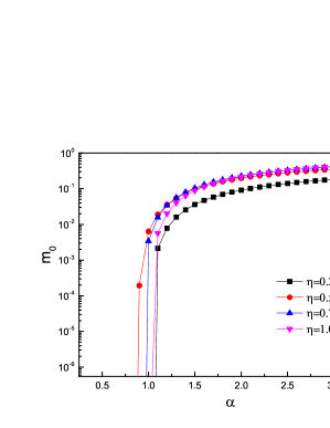
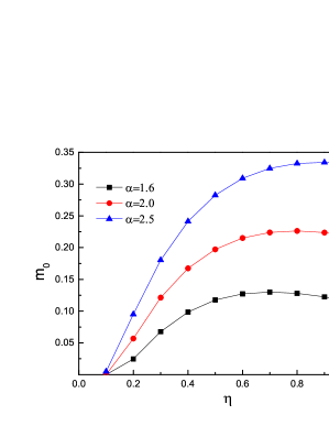
Figure 1: (a) The $\alpha$-dependence of $m_{0}$ at different values of $\eta$; (b) The $\eta$-dependence of $m_{0}$ at different values of $\alpha$. Results are obtained under the instantaneous approximation.

From the above analysis, we immediately deduce that the effective Coulomb interaction in Na₃Bi and Cd₃As₂ is too weak to generate an excitonic gap, and that the exact zero-temperature ground state of these materials is semimetal, rather than excitonic insulator. Moreover, both Na₃Bi and Cd₃As₂ lie deep in the gapless semimetallic phase, as shown in Fig. 2(a). There is no detectable signature of excitonic insulating behavior in these two materials.

III.2 Khveshchenko approximation

We then numerically solve Eq. (LABEL:Eq:GapEquationKhveshchenko) and present the results in Fig. 3. The corresponding $\alpha$-$\eta$ phase diagram is given in Fig. 2(b). We observe that the basic results are qualitatively the same as those obtained under the instantaneous approximation. In particular, for any given value of $\eta$, there is always a critical value $\alpha_{c}$ beyond which a finite gap is generated, and the gap is a monotonously increasing function of $\alpha$ in the range of $\alpha>\alpha_{c}$. For a specific, sufficiently large $\alpha$, the gap exhibits a non-monotonic dependence on the velocity ratio $\eta$, with its maximum being reached at certain critical ratio $\eta_{m}$.

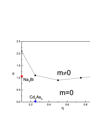
Figure 2: Phase diagram on the $\alpha$-$\eta$ plane. (a) Instantaneous approximation; (b) Khveshchenko approximation.

Although the conclusion is qualitatively the same, the quantitative results obtained under the Khveshchenko approximation are different from the instantaneous approximation. For instance, the critical value $\alpha_{c}\approx 1.5$ for $\eta=0.1$, and $\alpha_{c}\approx 0.9$ for $\eta=0.25$. In addition, $\alpha_{c}\approx 1.0$ for $\eta=1$. The smallest value of $\alpha_{c}$ appears at $\eta\approx 0.5$. Comparing Fig. 2(a) to Fig. 2(b), an apparent fact is that $\alpha_{c}$ obtained under the Khveshchenko approximation is generically slightly smaller than the one obtained under the instantaneous approximation. Once again, we conclude that Na₃Bi and Cd₃As₂ are both in the gapless semimetal phase.

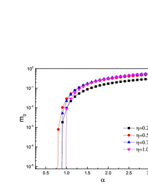
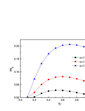
Figure 3: (a) The $\alpha$-dependence of $m_{0}$ at different values of $\eta$; (b) The $\eta$-dependence of $m_{0}$ at different values of $\alpha$. Results are obtained under the Khveshchenko approximation.

III.3 More suitable definitions of $\alpha$ and $\eta$

In the above analysis, we have defined the interaction strength and velocity ratio by $\alpha=\frac{e^{2}}{v_{\parallel}\epsilon_{0}\epsilon_{r}}$ and $\eta=\frac{v_{z}}{v_{\parallel}}$, respectively. These definitions were introduced and utilized in previous works Braguta16 ; Braguta17 . We would like to emphasize that these two definitions might not be appropriate Xiao17 . For instance, to examine the sole impact of the velocity anisotropy, one can fix the value of $\alpha$, which means $v_{\parallel}$ is simultaneously fixed, and tune the ratio $\eta$ by varying $v_{z}$. Because $v_{\parallel}$ is fixed and $v_{z}$ is varying, the total kinetic energy of 3D Dirac fermions are altered, and thus the effective strength of Coulomb interaction, which is determined by the ratio between the potential energy and the total kinetic energy, is also changed. Therefore, the Coulomb interaction is automatically tuned by varying $\eta$, though $\alpha$ remains fixed at a constant. As a consequence, the influences of the Coulomb interaction and the velocity anisotropy are entangled, and cannot be separated. In order to figure out how the Coulomb interaction and the velocity anisotropy separately affects dynamical gap generation, a more suitable choice is to define

$$\alpha^{*}=\frac{e^{2}}{\bar{v}\epsilon_{0}\epsilon_{r}}\quad\mathrm{and}\quad\eta^{*}=\frac{v_{z}}{v_{\parallel}},$$ (36)

where $\bar{v}=\sqrt[3]{v_{\parallel}^{2}v_{z}}$ represents a mean value of the fermion velocities. Now the two parameters $\alpha^{*}$ and $\eta^{*}$ can vary independently. Carrying out a simple transformation of the results expressed by $\alpha$ and $\eta$, we obtain a new phase diagram of 3D DSM depicted on the plane spanned by $\alpha^{*}$ and $\eta^{*}$, as shown by Fig. 4. We observe that, as the velocity anisotropy increases, the critical interaction strength grows dramatically. These results indicate that, the fermion velocity anisotropy tends to suppress gap generation, and the non-monotonic behavior shown in Fig. (1)b and Fig. (3)b originates from the competition between the increasing interaction strength and the growing velocity anisotropy. The suppression of dynamical gap generation by decreasing $\eta$ should be attributed to the enhanced dynamical screening of Coulomb interaction.

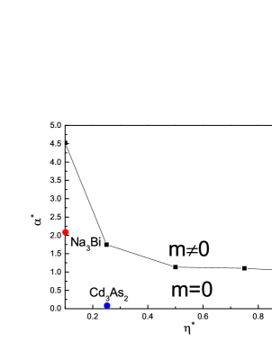
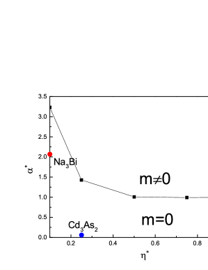
Figure 4: Phase diagram on the $\alpha^{*}$-$\eta^{*}$ plane. (a) Instantaneous approximation; (b) Khveshchenko approximation.

III.4 Impact of higher-order corrections

We have solved Eqs. (27)-(29) by setting $\eta=1$ and $N=2$. No dynamical gap is generated even when $\alpha\rightarrow\infty$. It is important to notice that the system contains two tuning parameters, namely $N$ and $\alpha$. Excitonic pairing occurs only when $N<N_{c}$ and $\alpha>\alpha_{c}$. If $N_{c}>2$, one can simply fix $N=2$ and then determine $\alpha_{c}$ by solving DS equations. However, if $N_{c}<2$, the Coulomb interaction cannot trigger excitonic pairing even in the $\alpha\rightarrow\infty$ limit. Actually, we find that $N_{c}\simeq 1.7$ in the limit $\alpha\rightarrow\infty$. It turns out that fermion velocity renormalization tends to suppress dynamical gap generation.

We emphasize here that the result $N_{c}<2$ is obtained by ignoring several potentially important effects, including the dynamical screening of Coulomb interaction, the wave-function renormalization, and the vertex correction, as evidenced by Eq. (26). Such a result might be changed considerably when these effects are taken into account. To determine the influence of these corrections, we have solved Eqs. (31)-(33) and find that $N_{c}\simeq 4.2$. For physical flavor $N=2$, the dependence of zero-energy gap $m_{0}$ on $\alpha$ is presented in Fig. 5, which clearly shows that $\alpha_{c}\simeq 3.0$. For Na₃Bi and Cd₃As₂, the fermion dispersion is strongly anisotropic and $\eta\ll 1$. According to the results given in Sec. III.3, the value of $\alpha_{c}$ will be further increased as $\eta$ decreases from $\eta=1$, which makes excitonic pairing more unlikely.

In order to calculate $\alpha_{c}$ and $N_{c}$ more accurately, it will be necessary to incorporate even more corrections, such as the feedback of fermion velocity renormalization and wave-function renormalization on the polarization function. Incorporating all these corrections is technically very involved, and will be studied in a separate work. According to the extensive calculations carried out by employing different approximations, it appears safe to conclude that Na₃Bi and Cd₃As₂ are both deep in the semimetallic phase, although more extensive calculations are needed to precisely determine $\alpha_{c}$ and $N_{c}$.

Figure 5: The $\alpha$-dependence of $m_{0}$ obtained after solving Eqs. (31)-(33) at $N=2$. The critical value $\alpha_{c}\simeq 3.0$.

IV Summary and Discussion

In summary, we have studied the stability of the semimetal ground state of 3D DSM against the long-range Coulomb interaction by making a DS equation analysis. To the leading order of $1/N$ expansion, we have solved the gap equation numerically and obtained a detailed phase diagram on the plane spanned by the Coulomb interaction strength and the velocity anisotropy parameter. Our results indicate that, while excitonic gap generation is promoted as the interaction becomes stronger, it is suppressed if the velocity anisotropy is enhanced. As a concrete application of our results, we have confirmed that the Coulomb interaction in Na₃Bi and Cd₃As₂ is not strong enough to open a dynamical gap. Thus, the semimetal ground state is very stable against Coulomb interaction. In fact, these two 3D DSMs lie deep in the gapless semimetal phase, hence the quantum fluctuation of excitonic pairing is ignorable and does not lead to any detectable effect.

We also have examined the impact of several higher-order corrections. In particular, we have incorporated the dynamical screening of Coulomb interaction, the fermion velocity renormalization, the wave-function renormalization, and the vertex correction into the DS equations. The new critical value $\alpha_{c}$ is quantitatively different from that obtained by retaining only the leading order of $1/N$ expansion. Nevertheless, the new $\alpha_{c}$ is still much larger than the physical value of $\alpha$ in Na₃Bi and Cd₃As₂, implying that these two materials are both robust gapless semimetals.

Recent Monte Carlo simulations Braguta16 ; Braguta17 reached distinct conclusions concerning the strict ground state of Na₃Bi and Cd₃As₂. A crucial difference between our results and those obtained Ref. Braguta16 and Ref. Braguta17 is in the chosen value of the dielectric constant. The relative dielectric constant $\epsilon_{r}$ was incorrectly missed in the calculations of Ref. Braguta16 and Ref. Braguta17 . In fact, if the dielectric constant of Na₃Bi and Cd₃As₂ are correctly chosen, the lattice simulation result could be consistent with our conclusion and also consistent with experiments.

It is interesting to search for the possible mechanism to promote dynamical gap generation in realistic 3D DSM materials. Since $\alpha\propto 1/(\bar{v}\epsilon_{r})$, the interaction will be made stronger if one finds an efficient way to decrease $\bar{v}$ and/or $\epsilon_{r}$. For 2D materials, the value of $\epsilon_{r}$ is strongly affected by the substrate. For example, $\epsilon_{r}\approx 2.8$ in graphene placed on SiO₂ substrate CastroNetoPhysics09 , but $\epsilon_{r}=1$ in suspended graphene. However, this scenario does not work in 3D DSMs, because changing the environment of a 3D material can hardly affect the value of the bulk $\epsilon_{r}$. Recent theoretical study Tang15 predicted that applying a uniform strain to graphene might enhance the Coulomb strength by reducing the Dirac fermion velocities. We speculate that this manipulation provides a promising method to reinforce the Coulomb interaction of Na₃Bi and Cd₃As₂. Another way to promote dynamical gap generation is to find more 3D DSM materials other than Na₃Bi and Cd₃As₂ that have smaller values of fermion velocities and smaller $\epsilon_{r}$.

The Coulomb interaction strength is $\alpha\approx 0.06$ in Cd₃As₂, which provides a small parameter to carry out ordinary perturbative expansion. Previous perturbative calculations Abrikosov70 ; Goswami11 ; Hosur12 ; Hofmann15 ; Throckmorton15 revealed that the fermion velocity grows with lowering energy, and that some observable quantities, including specific heat, compressibility, optical conductivity, and susceptibility, exhibit logarithmic-like dependence on energy or temperature. However, it is important to emphasize that, the perturbative expansion method cannot be used to compute the dynamical gap, because excitonic pairing is a genuine non-perturbative phenomenon and should be studied by means of non-perturbative tools, such as the DS equation approach and the quantum Monte Carlo simulation Braguta16 ; Braguta17 ; Karthik15 .

Appendix A Calculation of the polarization

We now provide the detailed calculation of the polarization function that appears in the dressed Coulomb interaction function Eq. (7).

The free fermion propagator for massless Dirac fermion is given by

$$G(\omega,\mathbf{k})=\frac{1}{\omega\gamma_{0}+v_{\parallel}(\gamma_{1}k_{x}+\gamma_{2}k_{y})+v_{z}\gamma_{3}k_{z}}.$$ (37)

To the leading order of $1/N$ expansion, the polarization function is defined as

$$\Pi(\Omega,q_{x},q_{y},q_{z}) = N\int\frac{d\omega}{2\pi}\frac{d^{3}\mathbf{k}}{(2\pi)^{3}}\mathrm{Tr}\left[\gamma_{0}G(\Omega,\mathbf{k})\gamma_{0}G\left(i(\omega+\Omega),\mathbf{k}+\mathbf{q}\right)\right],$$ (38)

where $N$ is the fermion flavor. Substituting Eq. (37) into Eq. (38), we obtain

$$\Pi\left(\Omega,\frac{q_{x}}{v_{\parallel}},\frac{q_{y}}{v_{\parallel}},\frac{q_{z}}{v_{z}}\right) = \frac{4N}{v_{\parallel}^{2}v_{z}}\int\frac{d\omega}{2\pi}\frac{d^{3}\mathbf{k}}{(2\pi)^{3}}\frac{\omega(\omega+\Omega)-\mathbf{k}\cdot(\mathbf{k}+\mathbf{q})}{\left(\omega^{2}+\mathbf{k}^{2}\right)\left[(\omega+\Omega)^{2}+\left|\mathbf{k}+\mathbf{q}\right|^{2}\right]},$$ (39)

where we have used the following transformations

$$v_{\parallel}k_{x}\rightarrow k_{x},\quad v_{\parallel}k_{y}\rightarrow k_{y},\quad v_{z}k_{z}\rightarrow k_{z},\quad v_{\parallel}q_{x}\rightarrow q_{x},\quad v_{\parallel}q_{y}\rightarrow q_{y},\quad v_{z}q_{z}\rightarrow q_{z}.$$ (40)

Making use of the Feynman parametrization formula

$$\frac{1}{AB}=\int_{0}^{1}dx\frac{1}{\left[xA+(1-x)B\right]^{2}},$$ (41)

we get

$$\Pi\left(\Omega,\frac{q_{x}}{v_{\parallel}},\frac{q_{y}}{v_{\parallel}},\frac{q_{z}}{v_{z}}\right) = \frac{4N}{v_{\parallel}^{2}v_{z}}\int_{0}^{1}dx\int\frac{d\omega}{2\pi}\frac{d^{3}\mathbf{k}}{(2\pi)^{3}}\frac{\omega(\omega+\Omega)-\mathbf{k}\cdot(\mathbf{k}+\mathbf{q})}{\left[\left(\omega+x\Omega\right)^{2}+|\mathbf{k}+x\mathbf{q}|^{2}+x(1-x)\left(\Omega^{2}+\mathbf{q}^{2}\right)\right]^{2}}.$$ (42)

We then re-define $\omega^{\prime}=\omega+x\Omega$ and $\mathbf{k}^{\prime}=\mathbf{k}+x\mathbf{q}$, and re-write the polarization in the form

$$\Pi\left(\Omega,\frac{q_{x}}{v_{\parallel}},\frac{q_{y}}{v_{\parallel}},\frac{q_{z}}{v_{z}}\right) = \frac{4N}{v_{\parallel}^{2}v_{z}}\int_{0}^{1}dx\int\frac{d\omega^{\prime}}{2\pi}\frac{d^{3}\mathbf{k}^{\prime}}{(2\pi)^{3}}\frac{\omega^{\prime 2}-\mathbf{k}^{\prime 2}-x(1-x)\left(\Omega^{2}-\mathbf{q}^{2}\right)}{\left[\omega^{\prime 2}+\mathbf{k}^{\prime 2}+x(1-x)\left(\Omega^{2}+\mathbf{q}^{2}\right)\right]^{2}}.$$ (43)

After carrying out the integration over $\omega^{\prime}$ and momenta, we get

$$\Pi\left(\Omega,\frac{q_{x}}{v_{\parallel}},\frac{q_{y}}{v_{\parallel}},\frac{q_{z}}{v_{z}}\right) = \frac{2N\mathbf{q}^{2}}{v_{\parallel}^{2}v_{z}}\int_{0}^{1}dxx(1-x)\int\frac{d^{3}\mathbf{k}^{\prime}}{(2\pi)^{3}}\frac{1}{\left[\mathbf{k}^{\prime 2}+x(1-x)\left(\Omega^{2}+\mathbf{q}^{2}\right)\right]^{3/2}}$$ (44)

$$= \frac{2N\mathbf{q}^{2}}{\pi^{2}v_{\parallel}^{2}v_{z}}F,$$

where

$$F = \left\{\frac{1}{12}\ln\left(\frac{2\Lambda+\sqrt{4\Lambda^{2}+\left(\Omega^{2}+\mathbf{q}^{2}\right)}}{\sqrt{\Omega^{2}+\mathbf{q}^{2}}}\right)-\int_{0}^{\frac{1}{2}}dxx(1-x)\frac{\Lambda}{\sqrt{\Lambda^{2}+x(1-x)\left(\Omega^{2}+\mathbf{q}^{2}\right)}}\right.$$ (45)

$$-\frac{1}{12}\int_{0}^{\frac{1}{2}}dx\left(3x^{2}-2x^{3}\right)\frac{(1-2x)\left(\Omega^{2}+\mathbf{q}^{2}\right)}{\left[\Lambda+\sqrt{\Lambda^{2}+x(1-x)\left(\Omega^{2}+\mathbf{q}^{2}\right)}\right]\sqrt{\Lambda^{2}+x(1-x)\left(\Omega^{2}+\mathbf{q}^{2}\right)}}$$

$$\left.+\frac{1}{12}\int_{0}^{\frac{1}{2}}dx\left(3x^{2}-2x^{3}\right)\frac{(1-2x)\left(\Omega^{2}+\mathbf{q}^{2}\right)}{x(1-x)\left(\Omega^{2}+\mathbf{q}^{2}\right)}\right\}.$$

In the regime $\sqrt{\Omega^{2}+\mathbf{q}^{2}}\ll\Lambda$, we retain only the leading term, i.e.,

$$\Pi\left(\Omega,\frac{q_{x}}{v_{\parallel}},\frac{q_{y}}{v_{\parallel}},\frac{q_{z}}{v_{z}}\right)=\frac{N\mathbf{q}^{2}}{6\pi^{2}v_{\parallel}^{2}v_{z}}\ln\left(\frac{\Lambda}{\sqrt{\Omega^{2}+\mathbf{q}^{2}}}\right).$$ (46)

Introducing the re-definitions $q_{x}\rightarrow v_{\parallel}q_{x}$, $q_{y}\rightarrow v_{\parallel}q_{y}$, $q_{z}\rightarrow v_{z}q_{z}$, and $\Lambda\rightarrow\left(v_{\parallel}^{2}v_{z}\right)^{1/3}\Lambda$, we have

$$\Pi(\Omega,q_{\parallel},q_{z})=\frac{N\left(v_{\parallel}^{2}q_{\parallel}^{2}+v_{z}^{2}q_{z}^{2}\right)}{6\pi^{2}v_{\parallel}^{2}v_{z}}\ln\left(\frac{\left(v_{\parallel}^{2}v_{z}\right)^{1/3}\Lambda}{\sqrt{\Omega^{2}+v_{\parallel}^{2}q_{\parallel}^{2}+v_{z}^{2}q_{z}^{2}}}\right).$$ (47)

Dynamical gap generation is a low-energy phenomenon, and the dominant contribution to the gap equation comes from the small enegy/momenta regime. Although the contribution from high energy/momenta regime is unimportant, the approximate polarization should be at least well-defined. We notice that the above approximate expression of $\Pi(\Omega,q_{\parallel},q_{z})$ is negative at very high energies, i.e., $\Omega\gg\left(v_{\parallel}^{2}v_{z}\right)^{1/3}\Lambda$, which would lead to a unphysical pole in the dressed Coulomb interaction function. The exact polarization is definitely always positive. Such unphysical pole originates from an improper approximation. In order to avoid the appearance of such pole, we make the following replacement

$$\ln\left(\frac{\left(v_{\parallel}^{2}v_{z}\right)^{1/3}\Lambda}{\sqrt{\Omega^{2}+v_{\parallel}^{2}q_{\parallel}^{2}+v_{z}^{2}q_{z}^{2}}}\right)\rightarrow\ln\left(\frac{\left(v_{\parallel}^{2}v_{z}\right)^{1/3}\Lambda+\sqrt{\Omega^{2}+v_{\parallel}^{2}q_{\parallel}^{2}+v_{z}^{2}q_{z}^{2}}}{\sqrt{\Omega^{2}+v_{\parallel}^{2}q_{\parallel}^{2}+v_{z}^{2}q_{z}^{2}}}\right).$$ (48)

Now the polarization becomes

$$\Pi(\Omega,q_{\parallel},q_{z})=\frac{N\left(v_{\parallel}^{2}q_{\parallel}^{2}+v_{z}^{2}q_{z}^{2}\right)}{6\pi^{2}v_{\parallel}^{2}v_{z}}\ln\left(\frac{\left(v_{\parallel}^{2}v_{z}\right)^{1/3}\Lambda+\sqrt{\Omega^{2}+v_{\parallel}^{2}q_{\parallel}^{2}+v_{z}^{2}q_{z}^{2}}}{\sqrt{\Omega^{2}+v_{\parallel}^{2}q_{\parallel}^{2}+v_{z}^{2}q_{z}^{2}}}\right).$$ (49)

This new polarization is very close to the exact polarization in the low energy/momenta regime, and meanwhile does not yield any unphysical pole in the high energy/momenta regime. We have used this approximate polarization in our DS equation calculations.

References

- (1) O. Vafek and A. Vishwanath, Annu. Rev. Condens. Matter Phys. 5, 83 (2014).
- (2) T. O. Wehling, A. M. Black-Schaffer, and A. V. Balatsky, Adv. Phys. 63, 1 (2014).
- (3) N. P. Armitage, E. J. Mele, and A. Vishwanath, Rev. Mod. Phys. 90, 015001 (2008).
- (4) S.-Y. Xu, Y. Xia, L. A. Wray, S. Jia, F. Meier, J. H. Dil, J. Osterwalder, B. Slomski, A. Bansil, H. Lin, R. J. Cava, and M. Z. Hasan, Science 332, 560 (2011).
- (5) T. Sato, K. Segawa, K. Kosaka, S. Souma, K. Nakayama, K. Eto, T. Minami, Y. Ando, and T. Takahashi, Nat. Phys. 7, 840 (2011).
- (6) L. Wu, M. Brahlek, R. V. Aguilar, A. V. Stier, C. M. Morris, Y. Lubashevsky, L. S. Bilbro, N. Bansal, S. Oh, and N. P. Armitage, Nat. Phys. 9, 410 (2013).
- (7) M. Brahlek, N. Bansal, N. Koirala, S.-Y. Xu, M. Neupane, C. Liu, M. Z. Hasan, and S. Oh, Phys. Rev. Lett. 109, 186403 (2012).
- (8) Z. Wang, Y. Sun, X.-Q. Chen, C. Franchini, G. Xu, H. Weng, X. Dai, and Z. Fang, Phys. Rev. B 85, 195320 (2012).
- (9) Z. Wang, H. Weng, Q. Wu, X. Dai, and Z. Fang, Phys. Rev. B 88, 125427 (2013).
- (10) Z. K. Liu, B. Zhou, Y. Zhang, Z. J. Wang, H. M. Weng, D. Prabhakaran, S.-K. Mo, Z. S. Shen, Z. Fang, X. Dai, Z. Hussain, and Y. L. Chen, Science 343, 864 (2014).
- (11) M. Neupane, S.-Y. Xu, R. Sankar, N. Alidoust, G. Bian, C. Liu, I. Belopolski, T.-R. Chang, H.-T. Jeng, H. Lin, A. Bansil, F. Chou, and M. Z. Hasan, Nat. Commun. 5, 3786 (2014).
- (12) Z. K. Liu, J. Jiang, B. Zhou, Z. J. Wang, Y. Zhang, H. M. Weng, D. Prabhakaran, S.-K. Mo, H. Peng, P. Dudin, T. Kim, M. Hoesch, Z. Fang, X. Dai, Z. X. Shen, D. L. Feng, Z. Hussain, and Y. L. Chen, Nat. Mat. 13, 677 (2014).
- (13) S. Borisenko, Q. Gibson, D. Evtushinsky, V. Zabolotnyy, B. Büchner, and R. J. Cava, Phys. Rev. Lett. 113, 027603 (2014).
- (14) L. P. He, X. C. Hong, J. K. Dong, J. Pan, Z. Zhang, J. Zhang, and S. Y. Li, Phys. Rev. Lett. 113, 246402 (2014).
- (15) A. H. Casto Neto, F. Guinea, N. M. R. Peres, K. S. Novoselov, and A. K. Geim, Rev. Mod. Phys. 81, 109 (2009).
- (16) V. N. Kotov, B. Uchoa, V. M. Pereira, F. Guinea, and A. H. Castro Neto, Rev. Mod. Phys. 84, 1067 (2012).
- (17) B. Yan and C. Felser, Annu. Rev. Condens. Matter Phys. 8, 337 (2017).
- (18) M. Z. Hasan, S.-Y. Xu, I. Belopolski, and S.-M. Huang, Annu. Rev. Condens. Matter Phys. 8, 289 (2017).
- (19) G. Xu, H. Weng, Z. Wang, X. Dai, and Z. Fang, Phys. Rev. Lett. 107, 186806 (2011).
- (20) C. Fang, M. J. Gilbert, X. Dai, and B. A. Bernevig, Phys. Rev. Lett. 108, 266802 (2012).
- (21) B.-J. Yang and N. Nagaosa, Nat. Commun. 5, 4898 (2014).
- (22) P. Goswami and S. Chakravarty, Phys. Rev Lett. 107, 196803 (2011).
- (23) P. Hosur, S. A. Parameswaran, and A. Vishwanath, Phys. Rev. Lett. 108, 046602 (2012).
- (24) J. Hofmann, E. Barnes, and S. Das Sarma, Phys. Rev. B 92, 045104 (2015).
- (25) R. E. Throckmorton, J. Hofmann, E. Barnes, and S. Das Sarma, Phys. Rev. B 92, 115101 (2015).
- (26) A. Sekine and K. Nomura, Phys. Rev. B 90, 075137 (2014).
- (27) J. González, Phys. Rev. B 90, 121107(R) (2014).
- (28) J. González, Phys. Rev. B 92, 125115 (2015).
- (29) V. V. Braguta, M. I. Katsnelson, A. Yu. Kotov, and A. A. Nikolaev, Phys. Rev. B 94, 205147 (2016)
- (30) V. V. Braguta, M. I. Katsnelson, and A. Yu. Kotov, arXiv:1704.07132v2.
- (31) A. H. Castro Neto, Physics 2, 30 (2009).
- (32) D. V. Khveshchenko, Phys. Rev. Lett. 87, 246802 (2001).
- (33) E. V. Gorbar, V. P. Gusynin, V. A. Miransky, and I. A. Shovkovy, Phys. Rev. B 66, 045108 (2002).
- (34) D. V. Khveshchenko and H. Leal, Nucl. Phys. B 687, 323 (2004).
- (35) G.-Z. Liu, W. Li, and G. Cheng, Phys. Rev. B 79, 205429 (2009).
- (36) D. V. Khveshchenko, J. Phys.:Condens. Matter 21, 075303 (2009).
- (37) O. V. Gamayun, E. V. Gorbar, and V. P. Gusynin, Phys. Rev. B 81, 075429 (2010).
- (38) J. Sabio, F. Sols, and F. Guinea, Phys. Rev. B 82, 121413(R) (2010).
- (39) G.-Z. Liu and J.-R. Wang, New J. Phys. 13, 033022 (2011).
- (40) J.-R. Wang and G.-Z. Liu, J. Phys. Condens. Matter 23, 155602 (2011).
- (41) J.-R. Wang and G.-Z. Liu, J. Phys. Condens. Matter 23, 345601 (2011).
- (42) J.-R. Wang and G.-Z. Liu, New J. Phys. 14, 043036 (2012).
- (43) C. Popovici, C. S. Fischer, and L. von Smekal, Phys. Rev. B 88, 205429 (2013).
- (44) J.-R. Wang and G.-Z. Liu, Phys. Rev. B 89, 195404 (2014).
- (45) M. E. Carrington, C. S. Fischer, L. von Smekal, and M. H. Thoma, Phys. Rev. B 94, 125102 (2016).
- (46) Fei Xue, and Xiao-Xiao Zhang, Phys. Rev. B 96, 195160 (2017)
- (47) A. Sharma, V. N. Kotov, and A. H. Castro Neto, Phys. Rev. B 95, 235124 (2017).
- (48) H.-X. Xiao, J.-R. Wang, H.-T. Feng, P.-L. Yin, and H.-S. Zong, Phys. Rev. B 96, 155114 (2017).
- (49) O. V. Gamayun, E. V. Gorbar, and V. P. Gusynin, Phys. Rev. B 80, 165429 (2009).
- (50) J. Wang, H. A. Fertig, G. Murthy, and L. Brey, Phys. Rev. B 83, 035404 (2011).
- (51) A. Katanin, Phys. Rev. B 93, 035132 (2016).
- (52) O. Vafek and M. J. Case, Phys. Rev. B 77, 033410 (2008).
- (53) J. González, Phys. Rev. B 82, 155404 (2010).
- (54) J. González, Phys. Rev. B 85, 085420 (2012).
- (55) J. E. Drut and T. A. Lähde, Phys. Rev. Lett. 102, 026802 (2009).
- (56) J. E. Drut and T. A. Lähde, Phys. Rev. B 79, 165425 (2009).
- (57) J. E. Drut and T. A. Lähde, Phys. Rev. B 79, 241405(R) (2009).
- (58) W. Armour, S. Hands, and C. Strouthos, Phys. Rev. B 81, 125105 (2010).
- (59) W. Armour, S. Hands, and C. Strouthos, Phys. Rev. B 84, 075123 (2011).
- (60) P. V. Buividovich and M. I. Polikarpov, Phys. Rev. B 86, 245117 (2012).
- (61) M. V. Ulybyshev, P. V. Buividovich, M. I. Katsnelson, and M. I. Polikarpov, Phys. Rev. Lett. 111, 056801 (2013).
- (62) D. Smith and L. von Smekal, Phys. Rev. B 89, 195429 (2014).
- (63) I. S. Tupitsyn and N. V. Prokof’ev, Phys. Rev. Lett. 118, 026403 (2017).
- (64) F. de Juan and H. A. Fertig, Solid State Commun. 152, 1460 (2012).
- (65) A. V. Kotikov and S. Teber, Phys. Rev. D 94, 114010 (2016).
- (66) C. D. Roberts and A. G. Williams, Prog. Part. Nucl. Phys. 33, 477 (1994).
- (67) D. C. Elias, R. V. Gorbachev, A. S. Mayorov, S. V. Morozov, A. A. Zhukov, P. Blake, L. A. Ponomarenko, I. V. Grigorieva, K. S. Novoselov, F. Guinea, and A. K. Geim, Nat. Phys. 7, 701 (2011).
- (68) A. S. Mayorov, D. C. Elias, I. S. Mukhin, S. V. Morozov, L. A. Ponomarenko, K. S. Novoselov, A. K. Geim, and R. V. Gorbachev, Nano. Lett. 12, 4629 (2012).
- (69) M. Hirata, K. Ishikawa, G. Matsuno, A. Kobayashi, K. Miyagawa, M. Tamura, C. Berthier, and K. Kanoda, Science 358, 1403 (2017).
- (70) T. Appelquist, D. Nash, and L. C. R. Wijewardhana, Phys. Rev. Lett. 60, 2575 (1988).
- (71) C. S. Fischer, R. Alkofer, T. Dahm, and P. Maris, Phys. Rev. D 70, 073007 (2004).
- (72) H.-T. Feng, F.-Y. Hou, X. He, W.-M. Sun, and H.-S. Zong, Phys. Rev. D 73, 016004 (2006).
- (73) H.-T. Feng, S. Shi, W.-M. Sun, and H.-S. Zong, Phys. Rev. D 86, 045020 (2012).
- (74) H.-T. Feng, B. Wang, W.-M. Sun, and H.-S. Zong, Phys. Rev. D 86, 105042 (2012).
- (75) J.-F. Li, H.-T. Feng, Y. Jiang, W.-M. Sun, and H.-S. Zong, Phys. Rev. D 87, 116008 (2013).
- (76) L. Janssen and I. F. Herbut, Phys. Rev. B 93, 165109 (2016).
- (77) V. P. Gusynin and P. K. Pyatkovskiy, Phys. Rev. D 94, 125009 (2016).
- (78) J.-R. Wang, G.-Z. Liu, and C.-J. Zhang, Phys. Rev. B 95, 075129 (2017).
- (79) M. E. Carrington, C. S. Fischer, L. von Smekal, and M. H. Thoma, Phys. Rev. B 97, 115411 (2018).
- (80) M. Dadsetani and A. Ebrahimian, J. of Electr. Mat. 45, 5867 (2016).
- (81) M. Zivitz and J. R. Stevenson, Phys. Rev. B 10, 2457 (1974).
- (82) J.-P. Jay-Gerin, M. J. Aubin, and L. Caron, Solid State Commun. 21, 771 (1977).
- (83) A. Mosca Conte, O. Pulci, and F. Bechstedt, Sci. Rep. 7, 45500 (2017).
- (84) H.-K. Tang, E. Laksono, J. N. B. Rodrigues, P. Sengupta, F. F. Assaad, and S. Adam, Phys. Rev. Lett. 115, 186602 (2015).
- (85) A. A. Abrikosov and S. D. Beneslavskii, Sov. Phys. JETP 32, 699 (1971).
- (86) N. Karthik and R. Narayanan, Phys. Rev. D 93, 045020 (2016); Phys. Rev. D 94, 065026 (2016); Phys. Rev. D 94, 045020 (2016); Phys. Rev. D 96, 054509 (2017).