Faber Approximation to the Mori-Zwanzig Equation

Abstract

We develop a new effective approximation of the Mori-Zwanzig equation based on operator series expansions of the orthogonal dynamics propagator. In particular, we study the Faber series, which yields asymptotically optimal approximations converging at least $R$-superlinearly with the polynomial order for linear dynamical systems. We provide a through theoretical analysis of the new method and present numerical applications to random wave propagation and harmonic chains of oscillators interacting on the Bethe lattice and on graphs with arbitrary topology.

1 Introduction

The Mori-Zwanzig (MZ) formulation is a technique from irreversible statistical mechanics that allows us to develop formally exact evolution equations for quantities of interest (phase space functions) in nonlinear dynamical systems. One of the main advantages of developing such exact equations is that they provide a theoretical starting point to avoid integrating the full dynamical system and solve directly for the quantities of interest, thus reducing the computational cost significantly. As an example, consider a large system of interacting particles, and suppose we are interested in studying the motion of one specific particle. By applying the MZ formulation to the equations of motion of the full particle system, it is possible extract a formally exact generalized Langevin equation (MZ equation) governing the position and the momentum of the particle of interest. This is at the basis of microscopic physical theories of Brownian motion [23, 6]. Computing the solution to the MZ equation is a very challenging task that relies on approximations and appropriate numerical schemes. One of the main difficulties is the approximation of the memory integral (convolution term), which encodes the effects of the so-called orthogonal dynamics in the observable of interest. The orthogonal dynamics is essentially a high-dimensional flow that satisfies a complex integro-differential equation. In statistical systems far from equilibrium, such flow has the same order of magnitude and dynamical properties as the observable of interest, i.e., there is no scale separation between the observable of interest and the orthgonal dynamics. In these cases, the computation of the MZ memory can be addressed only by problem-class-dependent approximations. The first effective technique to approximate the MZ memory integral was developed by H. Mori in [34]. The method relies on on continued fraction expansions, and it can be conveniently formulated in terms of recurrence relations [42, 24, 28, 29, 17]. The continued fraction expansion method of Mori made it possible to compute the exact solution to important prototype problems in statistical mechanics, such as the dynamics of the auto-correlation function of a tagged oscillator in an harmonic chain [15, 26]. Other effective approaches to approximate the MZ memory integral rely on perturbation methods [50, 39, 49], mode coupling techniques, [1, 41, 40], or functional approximation methods [19, 21, 35]. In a parallel effort, the applied mathematics community has, in recent years, attempted to derive general easy-to-compute representations of the MZ memory integral [48, 38, 20]. In particular, various approximations such as the $t$-model [8, 10, 43, 7], hierarchical perturbation methods [45, 51, 49], and data-driven methods [30] were proposed to address approximation of the MZ memory integral in situations where there is no clear separation of scales between the resolved and the unresolved dynamics.

In this paper, we study a new approximation of the MZ equation based on global operator series expansions of the orthogonal dynamics propagator. In particular, we study the Faber series, which yields asymptotically optimal approximations converging at least $R$-superlinearly with the polynomial order. The advantages of expanding the orthogonal dynamics propagator in terms of globally defined operator series are similar to those we obtain when we approximate a smooth function in terms of orthogonal polynomials rather than Taylor series [22]. As we will see, the proposed MZ memory approximation method based on global operator series outperform in terms of accuracy and computational efficiency the hierarchical memory approximation techniques discussed in [51, 44], which are based on Taylor-type expansions.

This paper is organized as follows. In Section 2, we briefly review the MZ formulation, and discuss common choices of projection operators. In Section 3 we develop new series expansions of the MZ memory integral based on operator series of the orthogonal dynamics propagator. We also develop exact MZ equations for the mean and the auto-correlation function of an observable of interest, and determine their analytical solution through Laplace transforms. In Section 4 we perform a thorough convergence analysis of the memory approximation methods we propose in this paper. In Section 5 we demonstrate the accuracy and effectiveness of the Faber approximation of the Mori-Zwazig equation. Specifically, we study two-dimensional random waves in an annulus, and the velocity auto-correlation function of a tagged oscillator in harmonic chains interacting on the Bethe lattice and on graphs with arbitrary topology.

2 The Mori-Zwanzig Formulation

Consider the following nonlinear dynamical system evolving on a smooth manifold $\Gamma\subseteq\mathbb{R}^{N}$

$$\frac{d\bm{x}}{dt}=\bm{F}(\bm{x}),\qquad\bm{x}(0)=\bm{x}_{0}.$$ (1)

For simplicity, here we assume that $\Gamma=\mathbb{R}^{N}$. The dynamics of any scalar-valued phase space function $u:\Gamma\to\mathbb{R}$ (quantity of interest) can be expressed in terms of a semi-group of operators acting on the space of observables , i.e.,

$$u(\bm{x}(t))=e^{(t-s)\mathcal{L}}u(\bm{x}(s)),\quad\textrm{where}\quad\mathcal{L}u(\bm{x})=\bm{F}(\bm{x})\cdot\nabla u(\bm{x}).$$ (2)

The operator $e^{(t-s)\mathcal{L}}$ is known as Koopman operator [27]. The subspace of functions of $u(\bm{x})$ can be described conveniently by means of a projection operator $\mathcal{P}$, which selects from an arbitrary function $f(\bm{x})$ the part $\mathcal{P}f(\bm{x})$ which depends on $\bm{x}$ only through $u(\bm{x})$. The nature, mathematical properties and connections between $\mathcal{P}$ and the observable $u$ are discussed in detail in [12]. For now, it suffices to assume that $\mathcal{P}$ is a bounded linear operator, and that $\mathcal{P}^{2}=\mathcal{P}$. Also, we denote by $\mathcal{Q}=\mathcal{I}-\mathcal{P}$ the complementary projection, $\mathcal{I}$ being the identity operator. The MZ formalism describes the evolution of observables initially in the image of $\mathcal{P}$. Because the evolution of observables is governed by the semi-group $e^{t\mathcal{L}}$, we seek an evolution equation for $e^{t\mathcal{L}}\mathcal{P}$. By using the well-known Dyson identity

$$e^{t\mathcal{L}}=e^{t\mathcal{Q}\mathcal{L}}+\int_{0}^{t}e^{s\mathcal{L}}\mathcal{P}\mathcal{L}e^{(t-s)\mathcal{Q}\mathcal{L}}ds,$$ (3)

we obtain

$$\frac{d}{dt}e^{t\mathcal{L}}\mathcal{P}=e^{t\mathcal{L}}\mathcal{P}\mathcal{L}\mathcal{P}+e^{t\mathcal{Q}\mathcal{L}}\mathcal{Q}\mathcal{L}\mathcal{P}+\int_{0}^{t}e^{s\mathcal{L}}\mathcal{P}\mathcal{L}e^{(t-s)\mathcal{Q}\mathcal{L}}\mathcal{Q}\mathcal{L}\mathcal{P}ds.$$ (4)

By applying this equation to an element $u_{0}=u(\bm{x}(0))$ in the image of $\mathcal{P}$, we obtain the well-known MZ equation

$$\frac{\partial}{\partial t}e^{t\mathcal{L}}u_{0} =e^{t\mathcal{L}}\mathcal{PL}u_{0}+e^{t\mathcal{QL}}\mathcal{QL}u_{0}+\int_{0}^{t}e^{s\mathcal{L}}\mathcal{PL}e^{(t-s)\mathcal{QL}}\mathcal{QL}u_{0}ds.$$ (5)

We emphasize that equation (5) is completely equivalent to (2). Acting on the left with $\mathcal{P}$, yields the evolution equation for projected dynamics

$$\frac{\partial}{\partial t}\mathcal{P}e^{t\mathcal{L}}u_{0}=\mathcal{P}e^{t\mathcal{L}}\mathcal{PL}u_{0}+\int_{0}^{t}\mathcal{P}e^{s\mathcal{L}}\mathcal{PL}e^{(t-s)\mathcal{QL}}\mathcal{QL}u_{0}ds.$$ (6)

This equation may be interpreted as a mean field equation in the common situation where $\mathcal{P}$ is a conditional expectation. The two terms at the right hand side of (6) are often called streaming term and memory term, respectively.

2.1 Projection Operators

The natural choice for the projection operator in the Mori-Zwanzig formulation is a conditional expectation [12], i.e., a completely positive linear operator with suitable properties [47]. Such conditional expectation can be rigorously defined in the context of operator algebras and it can have different forms. Hereafter, we discuss the most important cases.

2.1.1 Chorin’s Projection

In a series of papers [8, 10, 9], A. J. Chorin and collaborators defined the following projection operator

$$\big{(}\mathcal{P}u\big{)}(\hat{\bm{x}}_{0})=\frac{\displaystyle\int_{-\infty}^{+\infty}u(\hat{\bm{x}}(t;\hat{\bm{x}}_{0},\tilde{\bm{x}}_{0}),\tilde{\bm{x}}(t;\hat{\bm{x}}_{0},\tilde{\bm{x}}_{0}))\rho_{0}(\hat{\bm{x}}_{0},\tilde{\bm{x}}_{0})d\tilde{\bm{x}}_{0}}{\displaystyle\int_{-\infty}^{+\infty}\rho_{0}(\hat{\bm{x}}_{0},\tilde{\bm{x}}_{0})d\tilde{\bm{x}}_{0}},$$ (7)

which represents a conditional expectation in the sense of classical probability theory. In equation (7), $\bm{x}(t;x_{0})$ denotes the flow map generated by (1), which we can split into resolved $\hat{\bm{x}}(t;\hat{\bm{x}}_{0},\tilde{\bm{x}}_{0})$ and unresoved $\tilde{\bm{x}}(t;\hat{\bm{x}}_{0},\tilde{\bm{x}}_{0})$ maps, $u(\bm{x})=u(\hat{\bm{x}},\tilde{\bm{x}})$ is the quantity of interest, and $\rho_{0}(\hat{\bm{x}}_{0},\tilde{\bm{x}}_{0})$ is the probability density function of the initial state $\bm{x}_{0}$. Alternatively, one can replace $\rho_{0}$ with the equilibrium distribution of the system $\rho_{eq}(\hat{\bm{x}},\tilde{\bm{x}})$, assuming it exists. Clearly, if $\bm{x}_{0}$ is deterministic then $\rho_{0}(\hat{\bm{x}}_{0},\tilde{\bm{x}}_{0})$ is a product of Dirac delta functions. On the other hand, if $\hat{\bm{x}}_{0}$ and $\tilde{\bm{x}}_{0}$ are statistically independent, i.e. $\rho_{0}(\hat{\bm{x}}_{0},\tilde{\bm{x}}_{0})=\hat{\rho}_{0}(\hat{\bm{x}}_{0})\tilde{\rho}_{0}(\tilde{\bm{x}}_{0})$, then the conditional expectation (7) simplifies to

$$\big{(}\mathcal{P}u\big{)}(\hat{\bm{x}}_{0})=\int_{-\infty}^{+\infty}u(\hat{\bm{x}}(t;\hat{\bm{x}}_{0},\tilde{\bm{x}}_{0}),\tilde{\bm{x}}(t;\hat{\bm{x}}_{0},\tilde{\bm{x}}_{0}))\tilde{\rho}_{0}(\tilde{\bm{x}}_{0})d\tilde{\bm{x}}_{0}.$$ (8)

In the special case where $u(\hat{\bm{x}},\tilde{\bm{x}})=\hat{\bm{x}}(t;\hat{\bm{x}}_{0},\tilde{\bm{x}}_{0})$ we have

$$\big{(}\mathcal{P}\hat{\bm{x}}\big{)}(\hat{\bm{x}}_{0})=\int_{-\infty}^{+\infty}\hat{\bm{x}}(t;\hat{\bm{x}}_{0},\tilde{\bm{x}}_{0})\tilde{\rho}_{0}(\tilde{\bm{x}}_{0})d\tilde{\bm{x}}_{0},$$ (9)

i.e. the conditional expectation of the resolved variables $\hat{\bm{x}}(t)$ given the initial condition $\hat{\bm{x}}_{0}$. This means that an integration of (9) with respect to $\hat{\rho}_{0}(\hat{\bm{x}}_{0})$ yields the mean of the resolved variables

$$\left<\hat{\bm{x}}(t)\right>_{\rho_{0}}=\int_{-\infty}^{\infty}\big{(}\mathcal{P}\hat{\bm{x}}\big{)}(\hat{\bm{x}}_{0})\hat{\rho}_{0}(\hat{\bm{x}}_{0})d\hat{\bm{x}}_{0}=\int_{-\infty}^{\infty}\hat{\bm{x}}(t,\bm{x}_{0})\rho_{0}(\bm{x}_{0})d\bm{x}_{0}.$$ (10)

Obviously, if the resolved variables $\hat{\bm{x}}(t)$ evolve from a deterministic initial state $\hat{\bm{x}}_{0}$ then the conditional expectation (9) represents the average of the reduced-order flow map $\hat{\bm{x}}(t;\hat{\bm{x}}_{0},\tilde{\bm{x}}_{0})$ with respect to the PDF of $\tilde{\bm{x}}_{0}$, i.e.,

$$\bm{X}_{0}(t;\hat{\bm{x}}_{0})=\int_{-\infty}^{+\infty}\hat{\bm{x}}(t;\hat{\bm{x}}_{0},\tilde{\bm{x}}_{0})\tilde{\rho}_{0}(\tilde{\bm{x}}_{0})d\tilde{\bm{x}}_{0}.$$ (11)

In this case, the MZ equation (6) is an unclosed evolution equation (PDE) for the averaged flow map (11).

2.1.2 Mori’s Projection

Another definition of projection operator widely used in statistical mechanics is Mori’s projection [52]

$$\mathcal{P}u=\sum_{i=1}^{M}\frac{\langle u,\phi_{i}\rangle_{eq}}{\langle\phi_{i},\phi_{i}\rangle_{eq}}\phi_{i}(u(\bm{x})).$$ (12)

Here $\{\phi_{1},\phi_{2},...\}$ is an orthogonal basis that spans the Hilbert space of observables, i.e., functions of $u(\bm{x})$ (assuming that such space is indeed a Hilbert space). Orthogonality of $\{\phi_{j}\}$ is with respect to the inner product

$$\langle a,b\rangle_{eq}=\int\rho_{eq}(\bm{x})a(\bm{x})b(\bm{x})d\bm{x},$$ (13)

where $a(\bm{x})$, $b(\bm{x})$ are two arbitrary phase space functions, while $\rho_{eq}$ is the equilibrium distribution function of the system, assuming it exists. In the context of Hamiltonian statistical mechanics the phase variables are $\bm{x}=(\bm{p},\bm{q})$, where $\bm{q}$ are generalized coordinates while $\bm{p}$ are kinetic momenta. In this setting the natural choice for $\rho_{eq}$ is the canonical Gibbs distribution

$$\rho_{eq}(\bm{p},\bm{q})=\frac{1}{Z}e^{-\beta H(\bm{p},\bm{q})},$$ (14)

where $H(\bm{p},\bm{q})$ denotes the Hamiltonian of the system, and $Z$ is the partition function.

2.1.3 Berne’s Projection

A simpler projection operator was proposed by Berne in [3] (see also [42], p. 30). The standard form is

$$\mathcal{P}(\cdot)=\frac{\langle u_{0},(\cdot)\rangle_{eq}}{\langle u_{0},u_{0}\rangle_{eq}}u_{0}.$$ (15)

This projection can be considered as a subcase of the Mori projection (12). Note that by using Berne’s projection we can easily represent the auto-correlation function the observable $u(\bm{x}(t))$ as

$$C_{u}(t)=\frac{\langle u(t),u_{0}\rangle_{eq}}{\langle u_{0},u_{0}\rangle_{eq}}=\frac{\langle\mathcal{P}u(\bm{x}(t)),u_{0}\rangle_{eq}}{\langle u_{0},u_{0}\rangle_{eq}}.$$ (16)

3 Approximation of the Mori-Zwanzig Memory Integral

In this section, we develop new approximations of the Mori-Zwanzig memory integral

$$\int_{0}^{t}\mathcal{P}e^{s\mathcal{L}}\mathcal{P}\mathcal{L}e^{(t-s)\mathcal{Q}\mathcal{L}}\mathcal{Q}\mathcal{L}u_{0}ds$$ (17)

based on series expansions of the orthogonal dynamics propagator $e^{t\mathcal{Q}\mathcal{L}}$ in the form

$$e^{t\mathcal{Q}\mathcal{L}}=\sum_{n=0}^{\infty}a_{n}(t)\Phi_{n}\left(\mathcal{Q}\mathcal{L}\right),$$ (18)

where $\Phi_{n}$ are polynomial basis functions, and $a_{n}(t)$ are temporal modes. Series expansions in the form (18) can be rigorously defined in the context of matrix theory [31, 32], i.e., for operators $\mathcal{Q}\mathcal{L}$ between finite-dimensional vector spaces. The question of whether it is possible to extend such expansions to the infinite-dimensional case, i.e., for operators acting between infinite-dimensional Hilbert or Banach spaces, is not a trivial [11]. For example, it is known that the classical Taylor series

$$e^{t\mathcal{L}}=\sum_{k=0}^{\infty}\frac{t^{k}}{k!}\mathcal{L}^{k}$$ (19)

does not hold if $\mathcal{L}$ is an unbounded operator, e.g., the generator of the Koopman semigroup (2) (see [25], p. 481). In the latter case, $e^{t\mathcal{L}}$ should be properly defined as

$$e^{t\mathcal{L}}=\lim_{n\rightarrow\infty}\left(1-\frac{t\mathcal{L}}{n}\right)^{-n}.$$ (20)

In fact, $\left(1-t\mathcal{L}/n\right)^{-1}$ is the resolvent of $\mathcal{L}$ (apart from a constant factor), which can be defined for both bounded and unbounded linear operators. Despite the theoretical issues associated with the existence of convergent series expansions of semigroups generated by unbounded operators [14, 25], when it comes to computing we always need to discretize the system, most often by discretizing the generator of the semigroup. In this setting, $e^{t\mathcal{Q}\mathcal{L}}$ is truly a matrix exponential, where, with some abuse of notation, we denoted by $\mathcal{Q}$ and $\mathcal{L}$ the finite-dimensional representation of the operators $\mathcal{Q}$ and $\mathcal{L}$.

3.1 MZ-Dyson Expansion

Consider the classical Taylor series expansion of the orthogonal dynamics propagator

$$e^{t\mathcal{Q}\mathcal{L}}=\sum_{n=0}^{\infty}\frac{t^{n}}{n!}(\mathcal{Q}\mathcal{L})^{n}.$$ (21)

A substitution of this expansion into the MZ equation (6) yields

$$\frac{\partial}{\partial t}\mathcal{P}e^{t\mathcal{L}}u_{0} =\mathcal{P}e^{t\mathcal{L}}\mathcal{P}\mathcal{L}u_{0}+\int_{0}^{t}\mathcal{P}e^{s\mathcal{L}}\mathcal{P}\mathcal{L}e^{(t-s)\mathcal{Q}\mathcal{L}}\mathcal{Q}\mathcal{L}u_{0}ds,$$

$$=\mathcal{P}e^{t\mathcal{L}}\mathcal{P}\mathcal{L}u_{0}+\int_{0}^{t}\sum_{n=0}^{\infty}\frac{(t-s)^{n}}{n!}\underbrace{\mathcal{P}e^{s\mathcal{L}}\mathcal{P}\mathcal{L}(\mathcal{Q}\mathcal{L})^{n}\mathcal{Q}\mathcal{L}u_{0}}_{\mathcal{C}_{n}(s)u_{0}}ds,$$

$$=\mathcal{P}e^{t\mathcal{L}}\mathcal{P}\mathcal{L}u_{0}+\int_{0}^{t}\underbrace{\left[\sum_{n=0}^{\infty}\mathcal{C}_{n}(s)\frac{(t-s)^{n}}{n!}\right]}_{\mathcal{G}(t-s,s)}u_{0}ds,$$

$$=\mathcal{P}e^{t\mathcal{L}}\mathcal{P}\mathcal{L}u_{0}+\int_{0}^{t}\mathcal{G}(t-s,s)u_{0}ds,$$ (22)

where the memory operator $\mathcal{G}(t-s,s)$ is defined as

$$\mathcal{G}(t-s,s)=\sum_{n=0}^{\infty}\frac{(t-s)^{n}}{n!}\mathcal{C}_{n}(s),\qquad\mathcal{C}_{n}(s)=\mathcal{P}e^{s\mathcal{L}}\mathcal{P}\mathcal{L}(\mathcal{Q}\mathcal{L})^{n}\mathcal{Q}\mathcal{L},\quad n\geq 0.$$ (23)

We shall call this series expansion of the MZ equation as MZ-Dyson expansion. The reason for such definition is that (22) is equivalent to the $H$-model discussed in [51] and [44], which in turn is equivalent to a Dyson series expansion in the form

$$\frac{\partial}{\partial t}\mathcal{P}e^{t\mathcal{L}}u_{0} =\mathcal{P}e^{t\mathcal{L}}\mathcal{P}\mathcal{L}u_{0}+w_{0}(t)$$

where

$$w_{0}(t)= \int_{0}^{t}\mathcal{P}e^{s\mathcal{L}}\mathcal{PLQL}x_{0}ds+\int_{0}^{t}\int_{0}^{\tau_{1}}\mathcal{P}e^{s\mathcal{L}}\mathcal{PLQLQL}x_{0}dsd\tau_{1}$$

$$+...+\int_{0}^{t}\int_{0}^{\tau_{n-1}}...\int_{0}^{\tau_{1}}\mathcal{P}e^{s\mathcal{L}}\mathcal{PL}(\mathcal{QL})^{n}x_{0}dsd\tau_{1}...d\tau_{n-1}+...\,.$$ (24)

To prove such equivalence, we just need to prove that

$$\int_{0}^{t}\int_{0}^{\tau_{n-1}}...\int_{0}^{\tau}\mathcal{P}e^{s\mathcal{L}}\mathcal{P}\mathcal{L}(\mathcal{Q}\mathcal{L})^{n}dsd\tau_{1}...d\tau_{n-1}=\int_{0}^{t}\frac{(t-s)^{n-1}}{(n-1)!}\mathcal{P}e^{s\mathcal{L}}\mathcal{P}\mathcal{L}(\mathcal{Q}\mathcal{L})^{n}\mathcal{Q}\mathcal{L}ds.$$ (25)

We proceed by induction. To this end, we first define

$$\mathcal{A}_{n}(t)=\int_{0}^{t}\int_{0}^{\tau_{n-1}}...\int_{0}^{\tau}\mathcal{P}e^{s\mathcal{L}}\mathcal{P}\mathcal{L}(\mathcal{Q}\mathcal{L})^{n}dsd\tau_{1}...d\tau_{n-1},\qquad\mathcal{B}_{n}(t)=\int_{0}^{t}\frac{(t-s)^{n-1}}{(n-1)!}\mathcal{P}e^{s\mathcal{L}}\mathcal{P}\mathcal{L}(\mathcal{Q}\mathcal{L})^{n}\mathcal{Q}\mathcal{L}ds.$$ (26)

For $n=1$ we have $\mathcal{A}_{1}=\mathcal{B}_{1}$. For $n\geq 2$ we have $\mathcal{A}_{n}^{\prime}(t)=\mathcal{A}_{n-1}(t)$, $\mathcal{B}_{n}^{\prime}(t)=\mathcal{B}_{n-1}(t)$ and $\mathcal{A}_{n}(0)=\mathcal{B}_{n}(0)$. Hence, by induction we conclude that $\mathcal{A}_{n}(t)=\mathcal{B}_{n}(t)$, and therefore the memory integral in (22), with $\mathcal{G}$ given in (23), is equivalent to a Dyson series.

3.2 MZ-Faber Expansion

The Faber series of the orthogonal dynamics propagator $e^{t\mathcal{Q}\mathcal{L}}$ is an operator series in the form (see Appendix A)

$$e^{t\mathcal{Q}\mathcal{L}}=\sum_{j=0}^{\infty}a_{j}(t)\mathcal{F}_{j}(\mathcal{Q}\mathcal{L}),$$ (27)

where $\mathcal{F}_{j}$ is the $j-$th order Faber polynomial, and $a_{j}(t)$ are suitable temporal modes defined hereafter. The series expansion (27) is asymptotically optimal, in the sense that its $m$-th order truncation uniformly approximates the best sequence of operator polynomials converging to $e^{t\mathcal{Q}\mathcal{L}}$ as $m\rightarrow\infty$ [13]. A substitution of (27) into (17) yields the following expansion of the MZ equation (6)

$$\frac{\partial}{\partial t}\mathcal{P}e^{t\mathcal{L}}u_{0} =\mathcal{P}e^{t\mathcal{L}}\mathcal{P}\mathcal{L}u_{0}+\int_{0}^{t}\mathcal{P}e^{s\mathcal{L}}\mathcal{P}\mathcal{L}e^{(t-s)\mathcal{Q}\mathcal{L}}\mathcal{Q}\mathcal{L}u_{0}ds,$$

$$=\mathcal{P}e^{t\mathcal{L}}\mathcal{P}\mathcal{L}u_{0}+\int_{0}^{t}\sum_{j=0}^{\infty}a_{j}(t-s)\underbrace{\mathcal{P}e^{s\mathcal{L}}\mathcal{P}\mathcal{L}\mathcal{F}_{j}(\mathcal{Q}\mathcal{L})\mathcal{Q}\mathcal{L}u_{0}}_{\mathcal{C}_{j}(s)u_{0}}ds,$$

$$=\mathcal{P}e^{t\mathcal{L}}\mathcal{P}\mathcal{L}u_{0}+\int_{0}^{t}\mathcal{G}(t-s,s)u_{0}ds,$$ (28)

where

$$\mathcal{G}(t-s,s)=\sum_{j=0}^{\infty}a_{j}(t-s)\mathcal{C}_{j}(s),$$ (29)

and

$$a_{j}(t-s)=\frac{1}{2\pi i}\int_{|w|=R}\frac{e^{(t-s)\psi(w)}}{w^{j+1}}dw,\qquad\mathcal{C}_{j}(s)=\mathcal{P}e^{s\mathcal{L}}\mathcal{P}\mathcal{L}\mathcal{F}_{j}(\mathcal{Q}\mathcal{L})\mathcal{Q}\mathcal{L}.$$ (30)

Here, $\psi(w)$ is the conformal map at the basis of the Faber series (see Appendix A). The coefficients of the Laurent expansion of $\psi$ determine the recurrence relation of the Faber polynomials. High-order Laurent series usually yield higher convergence rates, but complicated recurrence relations (see equation (A)). Moreover, the computation of the integrals in (30) can be quite cumbersome if high-order Laurent series are employed. To avoid such drawbacks, in this paper we choose the conformal map $\psi(w)=w+c_{0}+c_{1}/w$. This yields the following expression for the coefficients $a_{j}(t-s)$

$$a_{j}(t-s)=\frac{e^{(t-s)c_{0}}}{(\sqrt{-c_{1}})^{j}}J_{j}\left(2(t-s)\sqrt{-c_{1}}\right),$$ (31)

where $J_{j}$ denotes the $j-$th Bessel function of the first kind. In Section 4 we prove that the Faber expansion of the MZ memory integral converges for any linear dynamical system and any finite integration time with rate that is at least $R$-superlinear.

Remark

The MZ-Dyson expansion we discussed in Section 3.1 is a subcase of the Faber expansion. In fact, Faber polynomials $\mathcal{F}_{j}(\mathcal{Q}\mathcal{L})$ corresponding to the conformal mapping $\psi(w)=w$ are simply monomials $(\mathcal{Q}\mathcal{L})^{j}$ (see Appendix A). Moreover, the temporal modes (31) reduce to $(t-s)^{j}/j!$ if we set $c_{0}=0$ and take the limit $c_{1}\rightarrow 0$.

3.3 Other Series Expansions of the MZ-Memory Integral

The operator exponential $e^{t\mathcal{Q}\mathcal{L}}$ (propagator of the orthogonal dynamics) can be expanded relative to basis functions other than Faber polynomials [31, 32]. This yields different approximations of the MZ memory integral and, correspondingly, different expansions of the MZ equation. Hereafter we discuss two relevant cases.

3.3.1 MZ-Lagrange Expansion

The MZ-lagrange expansion is based on the following semigroup expansion

$$e^{t\mathcal{Q}\mathcal{L}}=\sum_{j=1}^{n}e^{\lambda_{j}t}\prod_{\begin{subarray}{c}k=1\\ k\neq j\end{subarray}}^{n}\frac{(\mathcal{Q}\mathcal{L}-\lambda_{k}\mathcal{I})}{(\lambda_{j}-\lambda_{k})},$$ (32)

where $\{\lambda_{1},...,\lambda_{n}\}=\sigma(\mathcal{Q}\mathcal{L})$ is the spectrum of the matrix representation of the operator $\mathcal{Q}\mathcal{L}$ (eigenvalues counted with their multiplicity). Note that (32) is in the form (18) with

$$a_{j}(t)=e^{\lambda_{j}t},\quad\textrm{and}\quad\Phi_{j}(\mathcal{Q}\mathcal{L})=\prod_{\begin{subarray}{c}k=1\\ k\neq j\end{subarray}}^{n}\frac{(\mathcal{Q}\mathcal{L}-\lambda_{k}\mathcal{I})}{(\lambda_{j}-\lambda_{k})}.$$ (33)

A substitution of (32) into the MZ equation yields the MZ-Lagrange expansion

$$\frac{\partial}{\partial t}\mathcal{P}e^{t\mathcal{L}}u_{0}=\mathcal{P}e^{t\mathcal{L}}\mathcal{P}\mathcal{L}u_{0}+\int_{0}^{t}\mathcal{G}(t-s,s)u_{0}ds,$$ (34)

where

$$\mathcal{G}(t-s,s)=\sum_{j=1}^{n}e^{(t-s)\lambda_{j}}\mathcal{C}_{j}(s),\quad\textrm{and}\quad\mathcal{C}_{j}(s)=\mathcal{P}e^{s\mathcal{L}}\mathcal{P}\mathcal{L}\prod_{\begin{subarray}{c}k=1\\ k\neq j\end{subarray}}^{n}\frac{(\mathcal{Q}\mathcal{L}-\lambda_{k}\mathcal{I})}{(\lambda_{j}-\lambda_{k})},\qquad j\geq 1.$$ (35)

3.3.2 MZ-Newton Expansion

The MZ-Newton expansion is based on the following semigroup expansion

$$e^{t\mathcal{Q}\mathcal{L}}=f_{1,1}(t)\mathcal{I}+\sum_{j=2}^{n}f_{1,j}(t)\prod_{k=1}^{j-1}(\mathcal{Q}\mathcal{L}-\lambda_{k}\mathcal{I}),$$ (36)

where $f_{1,j}(t)$ is the divided difference defined recursively by

$$f_{1,j}(t)=\begin{dcases}e^{\lambda_{1}t}\quad&j=1,\\ \displaystyle\frac{e^{t\lambda_{1}}-e^{t\lambda_{2}}}{\lambda_{1}-\lambda_{2}}\quad&j=2,\\ \displaystyle\frac{f_{1,j-1}(t)-f_{2,j}(t)}{\lambda_{1}-\lambda_{j}}\quad&j\geq 3.\end{dcases}$$ (37)

A substitution of the Newton expansion (36) into the MZ equation yields the following MZ-Newton expansion

$$\frac{\partial}{\partial t}\mathcal{P}e^{t\mathcal{L}}u_{0}=\mathcal{P}e^{t\mathcal{L}}\mathcal{P}\mathcal{L}u_{0}+\int_{0}^{t}\mathcal{G}(t-s,s)u_{0}ds,$$ (38)

where

$$\mathcal{G}(t-s,s)=\mathcal{C}_{1}(s)e^{(t-s)\lambda_{1}}+\sum_{j=2}^{n}\mathcal{C}_{j}(s)f_{1,j}(t),\quad\quad\mathcal{C}_{j}(s)=\begin{cases}\mathcal{P}e^{s\mathcal{L}}\mathcal{P}\mathcal{L}&\quad j=1\\ \displaystyle\mathcal{P}e^{s\mathcal{L}}\prod_{k=1}^{j-1}(\mathcal{P}\mathcal{L}\mathcal{Q}\mathcal{L}-\lambda_{k}\mathcal{PL})&\quad j\geq 2\end{cases}.$$ (39)

Mori-Zwanzig Memory Operator
$\displaystyle\mathcal{G}(t-s,s)=\sum_{j=0}^{\infty}h_{j}(t-s)\mathcal{C}_{j}(s)$

Type	Temporal bases $h_{j}(t)$	Operators $\mathcal{C}_{j}(s)$
MZ-Dyson	$\displaystyle\frac{t^{j}}{j!}$	$\mathcal{P}e^{s\mathcal{L}}\mathcal{P}\mathcal{L}(\mathcal{Q}\mathcal{L})^{j}\mathcal{Q}\mathcal{L}$
MZ-Faber	$\displaystyle e^{tc_{0}}\frac{J_{j}(2t\sqrt{-c_{1}})}{(\sqrt{-c_{1}})^{j}}$	$\mathcal{P}e^{s\mathcal{L}}\mathcal{P}\mathcal{L}\mathcal{F}_{j}(\mathcal{Q}\mathcal{L})\mathcal{Q}\mathcal{L}$
MZ-Lagrange	$\displaystyle e^{t\lambda_{j}}$	$\displaystyle\mathcal{P}e^{s\mathcal{L}}\mathcal{P}\mathcal{L}\prod_{\begin{subarray}{c}k=1\\ k\neq j\end{subarray}}^{n}\frac{(\mathcal{Q}\mathcal{L}-\lambda_{k}\mathcal{I})}{(\lambda_{j}-\lambda_{k})}$
MZ-Newton	$f_{1,j}(t)$	$\displaystyle\begin{dcases}\mathcal{P}e^{s\mathcal{L}}\mathcal{P}\mathcal{L}&\quad j=1\\ \displaystyle\mathcal{P}e^{s\mathcal{L}}\prod_{k=1}^{j-1}(\mathcal{P}\mathcal{L}\mathcal{Q}\mathcal{L}-\lambda_{k}\mathcal{PL})&\quad j\geq 2\end{dcases}$

Table 1: Series expansions of the Mori-Zwanzig memory operator. Here $J_{j}$ is the $j$th Bessel function of the first kind, $c_{0}$ and $c_{1}$ are real numbers, $f_{1,j}(t)$ are defined in (37), and $\lambda_{j}$ are the eigenvalues of any matrix representation of $\mathcal{Q}\mathcal{L}$.

Remark

All series expansion methods we considered so far aim at representing the memory integral in the Mori-Zwazing equation for the same phase space function. Therefore, such series should be related to each other. Indeed, as shown in Table 1, they basically represent the same memory operator $\mathcal{G}(t-s,s)$ relative to different bases. This also means that the series can have different convergence rate. For example, as we will demonstrate numerically in Section 5 the MZ-Faber expansion converges much faster than the MZ-Dyson series.

3.4 Generalized Langevin Equation

We have seen in Section 3 that expanding the orthogonal dynamics propagator $e^{t\mathcal{Q}\mathcal{L}}$ in an operator series in the form (18) yields the Mori-Zwanzig equation

$$\frac{\partial}{\partial t}\mathcal{P}e^{t\mathcal{L}}u_{0}=\mathcal{P}e^{t\mathcal{L}}\mathcal{P}\mathcal{L}u_{0}+\sum_{j=0}^{\infty}\int_{0}^{t}h_{j}(t-s)\mathcal{C}_{j}(s)u_{0}ds,$$ (40)

where $h_{j}(t-s)$ are temporal modes, and $\mathcal{C}_{j}(s)$ are operators defined in Table 1. For example, if we consider the MZ-Dyson expansion, we have

$$h_{j}(t-s)=\frac{(t-s)^{j}}{j!},\qquad\mathcal{C}_{j}(s)=\mathcal{P}e^{s\mathcal{L}}\mathcal{P}\mathcal{L}(\mathcal{Q}\mathcal{L})^{j}\mathcal{Q}\mathcal{L}.$$ (41)

Equation (40) is the exact generalized Langevin equation (GLE) governing the projected dynamics of a quantity of interest. Such equation has different forms depending on the choice of the projection operator $\mathcal{P}$. In particular, if we choose Chorin’s projection (7) then (40) is an equation for the conditional expectation of the quantity of interest. On the other hand, if we choose Berne’s projection (15) then (40) becomes an equation for the autocorrelation function of the quantity of interest.

3.4.1 Evolution Equation for the Conditional Expectation

If we consider Chorin’s projection (7), then (40) becomes an unclosed evolution equation for the conditional expectation of the quantity of interest (see Section 2.1). However, in the special case where the dynamical system (1) is linear and the quantity of interest is $u(\bm{x})=x_{1}(t)$, it can be shown that the evolution equation for the conditional expectation is closed. To this end, let us first recall that if $\mathcal{P}$ is Chorin’s projection and $u(\bm{x})=x_{1}$ then

$$\mathcal{P}e^{t\mathcal{L}}x_{1}(0)=\langle x_{1}(t)\rangle_{\rho_{0}}=\int x_{1}(t,\bm{x}_{0})\rho_{0}(\bm{x}_{0})d\bm{x}_{0}.$$

In this case, (40) reduces to

$$\frac{d}{dt}\langle x_{1}(t)\rangle_{\rho_{0}} =a\langle x_{1}(t)\rangle_{\rho_{0}}+b+\int_{0}^{t}g(t-s)\langle x_{1}(s)\rangle_{\rho_{0}}ds+\int_{0}^{t}f(t-s)ds,$$ (42)

where the constants $a$, $b$, the MZ memory kernel $g(t-s)$, and the function $f(t-s)$ are defined by

$$\mathcal{P}\mathcal{L}x_{1}(0)=ax_{1}(0)+b,\qquad g(t-s)=\sum_{j=0}^{\infty}g_{j}h_{j}(t-s),\qquad f(t-s)=\sum_{j=0}^{\infty}f_{j}h_{j}(t-s).$$ (43)

The coefficients $g_{j}$, $f_{j}$ and the temporal bases $h_{j}(t-s)$ appearing in the series expansions above depend on the series expansion of the orthogonal dynamics propagator $e^{t\mathcal{Q}\mathcal{L}}$. Specifically, $g_{j}$ and $f_{j}$ are determined by the equation

$$\mathcal{C}_{j}(s)x_{1}(0)=g_{j}\langle x_{1}(s)\rangle_{\rho_{0}}+f_{j},$$ (44)

while $h_{j}(t-s)$ and $\mathcal{C}_{j}(s)$ are defined in Table 1. To derive equation (44) we used the identity $\mathcal{P}e^{s\mathcal{L}}f_{j}=f_{j}$. In the case of MZ-Dyson and MZ-Faber expansions we explicitly obtain

$$\mathcal{P}\mathcal{L}(\mathcal{Q}\mathcal{L})^{j}\mathcal{Q}\mathcal{L}x_{1}(0)=g_{j}^{D}x_{1}(0)+f_{j}^{D},\qquad\qquad\mathcal{P}\mathcal{L}\mathcal{F}_{j}(\mathcal{Q}\mathcal{L})\mathcal{Q}\mathcal{L}x_{1}(0)=g_{j}^{F}x_{1}(0)+f_{j}^{F},$$ (45)

where the superscripts $D$ and $F$ stand for “Dyson” and “Faber”, respectively.

3.4.2 Evolution Equation for the Autocorrelation Function

If we choose the projection operator $\mathcal{P}$ to be Berne’s projection (15), then equation (40) becomes a closed evolution equation for the autocorrelation function $C_{u}(t)$ of the quantity of interest. Such equation has the form

$$\frac{dC_{u}(t)}{dt}=aC_{u}(t)+\int_{0}^{t}g(t-s)C_{u}(s)ds,$$ (46)

where $a$ and $g$ are defined as

$$\mathcal{P}\mathcal{L}u_{0}=au_{0},\qquad g(t-s)=\sum_{j=0}^{\infty}g_{j}h_{j}(t-s).$$ (47)

As before, the temporal modes $h_{j}$ and the coefficients $g_{j}$ in the expansion of the MZ-memory kernel $g(t-s)$ depend on the expansion of the orthogonal dynamics propagator $e^{t\mathcal{Q}\mathcal{L}}$. Specifically, in the case of MZ-Dyson and MZ-Faber expansions we obtain, respectively,

$$\mathcal{P}\mathcal{L}(\mathcal{Q}\mathcal{L})^{j}\mathcal{Q}\mathcal{L}u_{0}=g_{j}^{D}u_{0},\qquad\mathcal{P}\mathcal{L}\mathcal{F}_{j}(\mathcal{Q}\mathcal{L})\mathcal{Q}\mathcal{L}u_{0}=g_{j}^{F}u_{0}.$$ (48)

It is worth noticing that Berne’s projection sends any function into the linear space spanned by the initial condition $u_{0}$.

3.4.3 Analytical Solution to the Generalized Langevin Equation

The analytical solution to the MZ equations (42) and (46) can be computed through Laplace transforms. To this end, let us first notice that both equations are in the form of a Volterra equation

$$\frac{dy(t)}{dt}=ay(t)+b+\int_{0}^{t}g(t-s)y(s)ds+\int_{0}^{t}f(t-s)ds.$$ (49)

Applying the Laplace transform

$$\mathscr{L}[\cdot](s)=\int_{0}^{\infty}(\cdot)e^{-st}dt$$ (50)

to both sides of (49) yields

$$sY(s)-y(0)=aY(s)+\frac{b}{s}+Y(s)G(s)+\frac{F(s)}{s},$$ (51)

i.e.,

$$Y(s)=\frac{(F(s)+b)/s+y(0)}{s-G(s)-a},$$ (52)

where

$$Y(s)=\mathscr{L}[y(t)],\qquad F(s)=\mathscr{L}[f(t)],\qquad G(s)=\mathscr{L}[g(t)].$$ (53)

Thus, the exact solution to the Volterra equation (49) can be written as

$$y(t)=\mathscr{L}^{-1}\left[\frac{(F(s)+b)/s+y(0)}{s-G(s)-a}\right].$$ (54)

The Laplace transform of the memory kernel $g(t)$, i.e., $G(s)$, can be computed analytically in many cases. For example, in the case of MZ-Dyson and MZ-Faber expansions we obtain, respectively

$$G(s)=\sum_{j=0}^{\infty}\frac{g^{D}_{j}}{s^{j+1}}\qquad\textrm{(MZ-Dyson),}$$ (55)

$$G(s)=\sum_{j=0}^{\infty}\frac{g^{F}_{j}}{2^{j}(\sqrt{-c_{1}})^{2j}}\frac{(\sqrt{s^{2}-4c_{1}}-s)^{j}}{\sqrt{s^{2}-4c_{1}}}\qquad\textrm{(MZ-Faber).}$$ (56)

The coefficients $g^{F}_{j}$ and $g^{D}_{j}$ are explicitly defined in (45), or (48), depending on whether we are interested in the mean or the correlation function of the quantity of interest.

Remark

The recurrence relation at the basis of the Faber polynomials (see equation (A)) induces a recurrence relation in the Laplace transform $G(s)$ of the MZ memory kernel. Therefore, a connection between the MZ-Faber approximation method we propose here and the method of recurrence relations of Lee [34, 29] can be established.

4 Convergence Analysis

In this section, we develop a thorough convergence analysis of the MZ-Faber expansion of the Mori-Zwanzig equation (6). The key theoretical results at the basis of our analysis can be found in our recent paper [51]. Here we focus, in particular, on high-dimensional linear systems in the form

$$\dot{\bm{x}}(t)=\bm{A}\bm{x}(t),\qquad\bm{x}(0)=\bm{x}_{0}(\omega),$$ (57)

where $\bm{x}_{0}(\omega)$ is a random initial state. Our goal is to prove that the norm of the approximation error

$$E_{n}(t) =\int_{0}^{t}\mathcal{P}e^{s\mathcal{L}}\mathcal{P}\mathcal{L}e^{(t-s)\mathcal{Q}\mathcal{L}}\mathcal{Q}\mathcal{L}u_{0}ds-\underbrace{\sum_{j=0}^{n}\int_{0}^{t}a_{j}(t-s)\mathcal{P}e^{s\mathcal{L}}\mathcal{P}\mathcal{L}\mathcal{F}_{j}(\mathcal{Q}\mathcal{L})\mathcal{Q}\mathcal{L}u_{0}ds}_{\textrm{MZ-Faber series}}$$

$$=\int_{0}^{t}\sum_{j=n+1}^{\infty}a_{j}(t-s)\mathcal{P}e^{s\mathcal{L}}\mathcal{P}\mathcal{L}\mathcal{F}_{j}(\mathcal{Q}\mathcal{L})\mathcal{Q}\mathcal{L}u_{0}ds$$ (58)

decays as we increase the polynomial order $n$, for any fixed integration time $t>0$, i.e.,

$$\lim_{n\rightarrow\infty}\left\|E_{n}(t)\right\|=0.$$

Throughout this Section $\left\|\cdot\right\|$ denotes either an operator norm, a norm in a function space or a standard norm in $\mathbb{C}^{N}$, depending on the context. The convergence proof of MZ-Faber series clearly depends on the choice of the projection operator and the phase space function $u(\bm{x})$ (quantity of interest). In this Section, we consider

$$u(\bm{x}(t))=x_{1}(t),$$ (59)

and Chorin’s projection (7). Similar results can be obtained for Berne’s projection. We begin with the following

Lemma 4.1.

Consider the linear dynamical system (57) and the phase space function (59). Then,

$$\mathcal{P}\mathcal{L}p_{k}(\mathcal{Q}\mathcal{L})\mathcal{Q}\mathcal{L}x_{1}(0) =\left[\bm{b}\cdot p_{k}(\bm{M}_{11}^{T})\bm{a}\right]x_{1}(0)+\left[p_{k}(\bm{M}_{11}^{T})\bm{M}_{11}^{T}\bm{a}\right]\cdot\langle\bm{x}_{-1}(0)\rangle_{\rho_{0}},$$

where $\mathcal{P}$ is Chorin’s projection (7), $\mathcal{Q}=\mathcal{I}-\mathcal{P}$, $\mathcal{L}=\bm{A}\bm{x}\cdot\nabla$, $p_{k}$ is an arbitrary polynomial of degree $k$,

$$\bm{x}_{-1}(0)=[x_{2}(0),x_{3}(0),\ldots,x_{N}(0)]^{T}\qquad\bm{a}=[A_{12},\dots,A_{1N}]^{T},\qquad\bm{b} =[A_{21},\dots,A_{N1}]^{T},$$

and $\bm{M}_{11}$ is the matrix obtained from $\bm{A}$ by removing the first row and the first column.

Proof.

By a direct calculation, it can be verified that

$$(\mathcal{Q}\mathcal{L})^{n}x_{1}(0) =\left[\left({\bm{M}}_{11}^{T}\right)^{n-1}\bm{a}\right]\cdot\left[\bm{x}_{-1}(0)-\langle\bm{x}_{-1}(0)\rangle_{\rho_{0}}\right],$$

$$\mathcal{L}(\mathcal{Q}\mathcal{L})^{n}x_{1}(0) =\left[\bm{b}^{T}\left({\bm{M}}_{11}^{T}\right)^{n-1}\bm{a}\right]x_{1}(0)+\left[\left({\bm{M}}_{11}^{T}\right)^{n}\bm{a}\right]\cdot\bm{x}_{-1}(0),$$

$$\mathcal{P}\mathcal{L}(\mathcal{Q}\mathcal{L})^{n}\mathcal{Q}\mathcal{L}x_{1}(0) =\left[\bm{b}^{T}\left(\bm{M}_{11}^{T}\right)^{n}\bm{a}\right]x_{1}(0)+\left[\left(\bm{M}_{11}^{T}\right)^{n}\bm{M}_{11}^{T}\bm{a}\right]\cdot\langle\bm{x}_{-1}(0)\rangle_{\rho_{0}}.$$ (60)

Note that each entry of the vector $\langle\bm{x}_{-1}(0)\rangle_{\rho_{0}}=[\langle x_{2}(0)\rangle_{\rho_{0}},...,\langle x_{N}(0)\rangle_{\rho_{0}}]^{T}$ is $\langle x_{i}(0)\rangle_{\rho_{0}}=\mathcal{P}x_{i}(0)$ ($i=2,...,N$). Thus, for any polynomial function in the form

$$p_{k}(\mathcal{Q}\mathcal{L})=\sum_{j=0}^{k}\beta_{k}(\mathcal{Q}\mathcal{L})^{j},$$ (61)

we have

$$\mathcal{P}\mathcal{L}p_{k}(\mathcal{Q}\mathcal{L})\mathcal{Q}\mathcal{L}x_{1}(0)= \sum_{j=0}^{k}\beta_{j}\mathcal{P}\mathcal{L}(\mathcal{Q}\mathcal{L})^{j}\mathcal{Q}\mathcal{L}x_{1}(0),$$

$$= \sum_{j=0}^{k}\beta_{j}\left(\left[\bm{b}^{T}\left(\bm{M}_{11}^{T}\right)^{n}\bm{a}\right]x_{1}(0)+\left[\left(\bm{M}_{11}^{T}\right)^{n}\bm{M}_{11}^{T}\bm{a}\right]\cdot\langle\bm{x}_{-1}(0)\rangle_{\rho_{0}}\right),$$

$$= \left[\bm{b}\cdot p_{k}\left(\bm{M}_{11}^{T}\right)\bm{a}\right]x_{1}(0)+\left[p_{k}\left(\bm{M}_{11}^{T}\right)\bm{M}_{11}^{T}\bm{a}\right]\cdot\langle\bm{x}_{-1}(0)\rangle_{\rho_{0}}.$$

This completes the proof of the Lemma.

$\Box$

To prove convergence of MZ-Faber series we need two more Lemmas involving Faber polynomials in the complex plane (see Appendix A).

Lemma 4.2.

Let $\gamma$ be the capacity of $\Omega\subseteq\mathbb{C}$. If $\Omega$ is symmetric with respect to the real axis, then for any $R>\gamma$ the conformal map (113) satisfies

$$\psi(R)\leq\psi(\gamma)+R-\frac{\gamma^{2}}{R}.$$

Proof.

We first notice that

$$\psi(R)=\psi(\gamma)+\int_{\gamma}^{R}\psi^{\prime}(t)dt.$$

By using Lemma 4.2 in [37], i.e.,

$$|\psi^{\prime}(t)|\leq 1+\left(\frac{\gamma}{|t|}\right)^{2},\quad|t|>\gamma$$

we have

$$\psi(R)-\psi(\gamma)\leq|\psi(R)-\psi(\gamma)|=\left|\int_{\gamma}^{R}\psi^{\prime}(t)dt\right|\leq\int_{\gamma}^{R}|\psi^{\prime}(t)|dt=R-\frac{\gamma^{2}}{R},$$

which completes the proof.

$\Box$

Next, consider an arbitrary matrix $\bm{A}$ and define the field value of $\bm{A}$ as

$$FV(\bm{A})=\left\{\bm{z}^{H}\bm{A}\bm{z}:\bm{z}\in\mathbb{C}^{N},\,\bm{z}^{H}\bm{z}=1\right\}.$$

The field value of $\bm{A}$ is a subset of the complex plane. Also, denote the truncated Faber series of the exponential matrix $e^{t\bm{A}}$ as

$$\bm{P}_{m}(t)=\sum_{j=0}^{m}a_{j}(t)\mathcal{F}_{j}(\bm{A}).$$ (62)

With this notation, we have the following

Lemma 4.3.

Let $\Omega\subset\mathbb{C}$ be symmetric with respect to the real axis, convex and with capacity $\gamma$. Consider an $N\times N$ matrix $\bm{A}$ with spectrum $\sigma(\bm{A})$, and an $N\times 1$ vector $\bm{v}$. If $\sigma(\bm{A})\subseteq\Omega$ and the field value $FV(\bm{A})\subseteq\Omega(q)$ for some $q\geq\gamma$, then the approximation error

$$\bm{e}_{m}(t-s)\bm{v}=e^{(t-s)\bm{A}}\bm{v}-\bm{P}_{(m-1)}(t-s)\bm{v}\qquad t\geq s$$

satisfies

$$\|\bm{e}_{m}(t-s)\bm{v}\|\leq C_{3}e^{(t-s)E}\left(\frac{qe^{t-s}}{m}\right)^{m-1}\quad m\geq 4q,$$

where

$$C_{3}=C_{3}(v)=8e\|\bm{v}\|q\left(1+\frac{1}{8q}\right)\quad\textrm{and}\quad E=1+\psi(\gamma).$$

Proof.

If $q\geq\gamma$ then we have, thanks to the convexity of $\Omega$ and the analyticity of the exponential function,

$$\|\bm{e}_{m}(t-s)\bm{v}\|\leq 8\|\bm{v}\|e\left(1+\frac{1}{8q}\right)m\left(\frac{q}{m}\right)^{m}\max_{|z|\in\Gamma(m)}\left|e^{(t-s)z}\right|\qquad m\geq 4q$$ (63)

(see Theorem 4.2 in [37]). On the other hand,

$$\max_{|z|\in\Gamma(m)}\left|e^{(t-s)z}\right|=e^{(t-s)\psi(m)}\qquad m\geq 4q.$$ (64)

By using Lemma 4.2 we have

$$\psi(m)\leq\psi(\gamma)+m-\frac{\gamma^{2}}{m}\leq\psi(\gamma)+m,$$ (65)

and therefore

$$e^{(t-s)\psi(m)}\leq e^{(t-s)(m-1)}e^{(t-s)(1+\psi(\gamma))}\quad m\geq 4q\geq\gamma.$$ (66)

Combining (63) , (64) and (66), we obtain

$$\|\bm{e}_{m}(t-s)\bm{v}\|\leq C_{3}\exp((t-s)E)\left(\frac{qe^{t-s}}{m}\right)^{m-1},$$ (67)

where

$$C_{3}=8e\|\bm{v}\|q\left(1+\frac{1}{8q}\right)\quad\textrm{and}\quad E=1+\psi(\gamma).$$

$\Box$

At this point, we we have all elements to prove the following

Theorem 4.4.

(Convergence of the MZ-Faber Expansion) Consider the linear dynamical system (57), the phase space function (59) and the projection operator (7). The norm of the approximation error (58) satisfies

$$\|E_{n}(t)\|\leq K\left(\frac{q}{n+1}\right)^{n}\frac{e^{t\beta}-e^{t(E+n)}}{\beta-E-n}\qquad t\geq 0,\quad n\geq 4q,$$ (68)

where $n$ is the Faber polynomial order, while $q$, $K$, $\beta$ and $E$ are suitable constants defined in the proof of the theorem.

Proof.

We aim at finding an upper bound for

$$\|E_{n}(t)\| =\left\|\int_{0}^{t}\mathcal{P}e^{s\mathcal{L}}\sum_{j=n+1}^{\infty}a_{j}(t-s)\mathcal{P}\mathcal{L}\mathcal{F}_{j}(\mathcal{Q}\mathcal{L})\mathcal{Q}\mathcal{L}x_{1}(0)ds\right\|.$$ (69)

To this end, we fist notice that quantity $\mathcal{F}_{j}(\mathcal{Q}\mathcal{L})\mathcal{Q}\mathcal{L}$ is a $(j+1)$-th order operator polynomial in $\mathcal{Q}\mathcal{L}$. Thus, we can apply Lemma 4.1 to obtain

$$\mathcal{P}\mathcal{L}\mathcal{F}_{j}(\mathcal{Q}\mathcal{L})\mathcal{Q}\mathcal{L}x_{1}(0)=\left[\bm{b}\cdot\mathcal{F}_{j}(\bm{M}_{11}^{T})\bm{a}\right]x_{1}(0)+\left[\mathcal{F}_{j}(\bm{M}_{11}^{T})\bm{M}_{11}^{T}\bm{a}\right]\cdot\langle\bm{x}_{-1}(0)\rangle_{\rho_{0}}.$$ (70)

Let us now set

$$\eta_{n}(t-s)=\left\|\sum_{j=n+1}^{\infty}a_{j}(t-s)\mathcal{P}\mathcal{L}\mathcal{F}_{j}(\mathcal{Q}\mathcal{L})\mathcal{Q}\mathcal{L}x_{1}(0)\right\|.$$ (71)

By using (70) and the Cauchy-Schwartz inequality we have

$$\eta_{n}(t-s)\leq C_{4}\left\|\sum_{j=n+1}^{\infty}a_{j}(t-s)\mathcal{F}_{j}({\bm{M}}_{11}^{T})\bm{a}\right\|+C_{5}\left\|\sum_{j=n+1}^{\infty}a_{j}(t-s)\mathcal{F}_{j}(\bm{M}_{11}^{T})\bm{M}_{11}^{T}\bm{a}\right\|,$$ (72)

where $C_{4}=\|\bm{b}^{T}\||x_{1}(0)|$, $C_{5}=\|\langle\bm{x}_{-1}(0)\rangle_{\rho_{0}}\|$. The two sums in (72) represent the error in the Faber approximation of the matrix exponential $e^{(t-s){\bm{M}}^{T}_{11}}$. In fact,

$$\bm{e}_{(n+1)}(t-s)=e^{(t-s){\bm{M}}^{T}_{11}}-\sum_{j=1}^{n}a_{j}(t-s)\mathcal{F}_{j}({\bm{M}}^{T}_{11})=\sum_{j=n+1}^{\infty}a_{j}(t-s)\mathcal{F}_{j}(\bm{M}^{T}_{11}).$$ (73)

Combining (69), (71), (72) and (67) yields

$$\|E_{n}(t)\| \leq\int_{0}^{t}\eta_{n}(t-s)\left\|\mathcal{P}e^{s\mathcal{L}}\right\|ds,$$

$$\leq\int_{0}^{t}\left(C_{4}\left\|\bm{e}_{(n+1)}(t-s)\bm{a}\right\|+C_{5}\left\|\bm{e}_{(n+1)}(t-s)\bm{M}_{11}^{T}\bm{a}\right\|\right)\|\mathcal{P}e^{s\mathcal{L}}\|ds,$$

$$\leq\int_{0}^{t}Ke^{s\beta}e^{(t-s)(E+n)}\left(\frac{q}{n+1}\right)^{n}ds,$$

$$\leq K\left(\frac{q}{n+1}\right)^{n}\frac{e^{t\beta}-e^{t(E+n)}}{\beta-E-n}\quad n\geq 4q.$$ (74)

Here we used the semigroup estimation $\|e^{s\mathcal{L}}\|\leq We^{s\beta}$. The constants in (74) are

$$K=\|\mathcal{P}\|C_{6}W,\qquad C_{6}=2\max\{C_{4}C_{3},C_{5}C_{3}^{*}\},\qquad E=1+\psi(\gamma),$$ (75)

where

$$C_{3}=8e\|\bm{a}\|q\left(1+\frac{1}{8q}\right),\qquad C_{3}^{*}=8e\|\bm{M}_{11}^{T}\bm{a}\|q\left(1+\frac{1}{8q}\right).$$ (76)

It can be shown that the upper bound (74) is always positive, and goes to zero as we send the Faber polynomial order $n$ to infinity. This implies that

$$\lim_{n\rightarrow\infty}\left\|E_{n}(t)\right\|=0,$$ (77)

i.e., the MZ-Faber expansion converges for any finite time $t\geq 0$. This completes the proof.

$\Box$

Next, we estimate the convergence rate of the MZ-Faber expansion. To this end, let us define

$$R(t,n)=K\left(\frac{q}{n+1}\right)^{n}\frac{e^{t\beta}-e^{t(E+n)}}{\beta-E-n},\quad n\geq 4q$$ (78)

the be the upper bound (74). We have the following

Corollary 4.4.1.

(Convergence Rate of the MZ-Faber Expansion) With the same the notation of Theorem 4.4, the MZ-Faber expansion converges at least $R$-superlinearly with the polynomial order, i.e.

$$\lim_{n\rightarrow\infty}\frac{R(t,n+1)}{R(t,n)}=0$$ (79)

for any finite time $t\geq 0$.

Proof.

By a direct calculation it is easy to verify that (79) holds true. In fact,

$$\frac{R(t,n+1)}{R(t,n)}=\frac{q}{n+2}\left(\frac{n+1}{n+2}\right)^{n}\frac{e^{t\beta}-e^{t(E+n+1)}}{e^{t\beta}-e^{t(n+E)}}\frac{\beta-E-n}{\beta-E-(n+1)}$$ (80)

Therefore,

$$\lim_{n\rightarrow+\infty}\frac{R(t,n+1)}{R(t,n)}=\lim_{n\rightarrow+\infty}\frac{qe^{t}}{n+2}\left(\frac{n+1}{n+2}\right)^{n}=0,\qquad t<\infty.$$ (82)

$\Box$

By using asymptotic analysis we can show theoretically that also the MZ-Dyson expansion converge $R$-superlinearly. To this end, let us define the MZ-Dyson approximation error

$$E_{n}(t)=\int_{0}^{t}\mathcal{P}e^{s\mathcal{L}}\mathcal{P}\mathcal{L}e^{(t-s)\mathcal{Q}\mathcal{L}}\mathcal{Q}\mathcal{L}u_{0}ds-\underbrace{\sum_{j=0}^{n}\int_{0}^{t}a_{j}(t-s)\mathcal{P}e^{s\mathcal{L}}\mathcal{P}\mathcal{L}(\mathcal{Q}\mathcal{L})^{j}\mathcal{Q}\mathcal{L}u_{0}ds}_{\textrm{MZ-Dyson series}}.$$ (83)

By following the same steps we used in the proof of Theorem 4.4, we can bound the norm of (83) as

$$\left\|E_{n}(t)\right\|\leq F(t,n).$$ (84)

where

$$F(t,n)=C\frac{(At)^{n}}{(n+1)!}\qquad A,C\geq 0.$$ (85)

Such upper bound plays the same role as $R(t,n)$ in the MZ-Faber expansion of $E_{n}(t)$ (see Eqs. (74) and (78)). Taking the ratio between $F(t,n+1)$ and $F(t,n)$ we obtain

$$\lim_{n\rightarrow\infty}\frac{F(t,n+1)}{F(t,n)}=\lim_{n\rightarrow\infty}\frac{At}{n+2}=0.$$ (86)

5 Numerical Examples

In this section, we demonstrate the accuracy and effectiveness of the MZ-Dyson and MZ-Faber expansion methods we developed in this paper in applications to prototype problems involving random wave propagation and harmonic chains of oscillators interacting on a Bethe lattice.

5.1 Random Wave Propagation

Consider the following initial/boundary value problem for the wave equation in an annulus with radii $r_{1}=1$ and $r_{2}=11$

$$\frac{\partial^{2}w}{\partial t^{2}}=\frac{\partial^{2}w}{\partial r^{2}}+\frac{1}{r}\frac{\partial w}{\partial r}+\frac{1}{r^{2}}\frac{\partial^{2}w}{\partial\theta^{2}},$$ (87)

where

$$w(t,r_{1},\theta)=0,\qquad w(t,r_{2},\theta)=0\qquad w(0,r,\theta)=w_{0}(r,\theta;\omega),\qquad\frac{\partial w(0,r,\theta)}{\partial t}=0.$$ (88)

The field $w(t,r,\theta)$ represents the wave amplitude at time $t$, while $w_{0}(r,\theta;\omega)$ is the wave field at initial time, which is set to be random. We seek the for an approximation of the solution $w(t,r,\theta)$ in the form

$$w_{N}(t,r,\theta)=\sum_{n=1}^{N}\widehat{w}_{n}(t)\psi_{n}(r,\theta),$$ (89)

where $\psi_{n}(r,\theta)$ are standard trigonometric functions. The random wave field at initial time is represented as

$$w_{0}(r,\theta;\omega)=\sum_{n=1}^{M}\widehat{w}_{n}(0)\psi_{n}(r,\theta),\qquad M\leq N,$$ (90)

where $\widehat{w}_{n}(0)$ are i.i.d Gaussian random variables. We substitute (89) into (87) and impose that the residual is orthogonal to the space spanned by the basis $\{\psi_{1},...,\psi_{N}\}$ [22]. This yields the linear system

$$\frac{d^{2}}{dt^{2}}\widehat{\bm{w}}(t)=\bm{A}\widehat{\bm{w}}(t),$$ (91)

where $\bm{A}$ is an $N\times N$ matrix with entries

$$A_{mn}=\frac{\displaystyle\int_{r_{1}}^{r_{2}}\int_{0}^{2\pi}\left(\frac{\partial^{2}\psi_{n}}{\partial r^{2}}+\frac{1}{r}\frac{\partial\psi_{n}}{\partial r}+\frac{1}{r^{2}}\frac{\partial^{2}\psi_{n}}{\partial\theta^{2}}\right)\psi_{m}drd\theta}{\displaystyle\int_{r_{1}}^{r_{2}}\int_{0}^{2\pi}\psi_{m}^{2}drd\theta}.$$ (92)

We are interested in building a convergent reduced-order model for the wave amplitude at a specific point within the annulus, e.g., where we placed a sensor. To this end, we transform the system (91) form the modal space to the nodal space defined by an interpolant of at $N$ collocation points. Such transformation can be easily defined by evaluating (89) at a set of distinct collocation nodes $\bm{x}_{n}=(r_{i(n)},\theta_{j(n)})$ ($n=1,...,N$) within the annulus. This yields

$$\bm{w}(t)=\bm{\Psi}\widehat{\bm{w}}(t),$$ (93)

where $\bm{w}(t)=[w(t,\bm{x}_{1}),...,w(t,\bm{x}_{N})]^{T}$, while $\bm{\Psi}$ is the $N\times N$ transformation matrix defined as

$$\bm{\Psi}=\left[\begin{matrix}\psi_{1}(\bm{x}_{1})&\dots&\psi_{N}(\bm{x}_{1})\\ \vdots&&\vdots\\ \psi_{1}(\bm{x}_{N})&\dots&\psi_{N}(\bm{x}_{N})\end{matrix}\right].$$

Differentiating (93) with respect to time we obtain

$$\frac{d^{2}}{dt^{2}}\bm{w}(t)=\bm{\Psi}\bm{A}\bm{\Psi}^{-1}\bm{w}(t).$$ (94)

This system evolves from the random initial state

$$\bm{w}(0)=\bm{\Psi}\widehat{\bm{w}}(0),\qquad\frac{d\bm{w}(0)}{dt}=0.$$ (95)

In Figure 1 we plot the mean solution of the random wave equation for initial conditions in the form (90) with different number of modes.

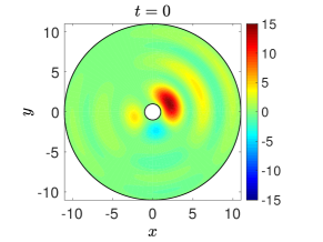
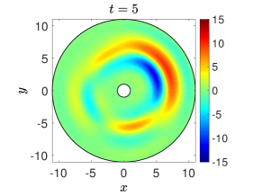
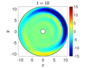
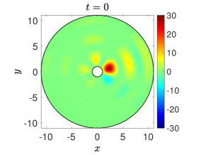
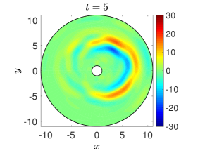
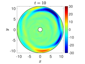
Figure 1: Mean solution of the random wave equation in the annulus. We consider two random initial conditions in the form (90), with different number of modes: $M=25$ (first row), $M=50$ (second row).

Generalized Langevin Equation for the Mean Wave Amplitude

We are interested in building a convergent reduced-order model for the mean wave amplitude at a specific point within the annulus, e.g., where we would like to place a sensor. Such a dynamical system can be constructed by using the Mori-Zwanzig formulation and Chorin’s projection operator (7). In particular, let us define the quantity of interest as $u(\bm{w})=w_{1}(t)$, i.e., the wave amplitude at the spatial point $(r,\theta)=(1.1,0.1)$. The exact evolution equation for mean of $w_{1}(t)$ was derived in Section 3.4.1, and it is rewritten hereafter for convenience

$$\frac{d}{dt}\langle w_{1}(t)\rangle_{\rho_{0}} =a\langle w_{1}(t)\rangle_{\rho_{0}}+b+\int_{0}^{t}g(t-s)\langle w_{1}(s)\rangle_{\rho_{0}}ds+\int_{0}^{t}f(t-s)ds.$$ (96)

We recall that

$$\mathcal{P}\mathcal{L}w_{1}(0)= B_{11}w_{1}(0)+\bm{a}\cdot\bm{\left missing}<\bm{w}_{-1}(0)\right>_{\rho_{0}}$$

$$= aw_{1}(0)+b,$$

and $\mathcal{L}=\left[\bm{\Psi}\bm{A}\bm{\Psi}^{-1}\bm{w}\right]\cdot\nabla$. The memory kernel $g(t-s)$ and the function $f(t-s)$ can be expanded by using in any of the operator series summarized in Table 1. For instance, if we employ MZ-Faber series we obtain

$$g(t-s)=\sum_{j=0}^{n}g^{F}_{j}e^{tc_{0}}\frac{J_{j}(2t\sqrt{-c_{1}})}{(\sqrt{-c_{1}})^{j}},\qquad f(t-s)=\sum_{j=0}^{n}f^{F}_{j}e^{tc_{0}}\frac{J_{j}(2t\sqrt{-c_{1}})}{(\sqrt{-c_{1}})^{j}}.$$ (97)

The coefficients $g_{j}^{F}$ and $f_{j}^{F}$ are explicitly obtained as

$$g_{j}^{F}=\bm{b}^{T}\mathcal{F}_{j}\left(\bm{M}_{11}^{T}\right)\bm{a},\qquad f_{j}^{F}=\left[\mathcal{F}_{j}\left(\bm{M}_{11}^{T}\right)\bm{M}_{11}^{T}\bm{a}\right]\cdot\langle\bm{w}_{-1}(0)\rangle_{\rho_{0}},$$ (98)

where

$$\bm{w}_{-1}(0)=[w_{2}(0),w_{3}(0),\ldots,w_{N}(0)]^{T},\qquad\bm{a}=[B_{12},\dots,B_{1N}]^{T},\qquad\bm{b} =[B_{21},\dots,B_{N1}]^{T},$$

$\bm{B}=\bm{\Psi}\bm{A}\bm{\Psi}^{-1}$ and $\bm{M}_{11}$ is the matrix obtained from $\bm{B}$ by removing the first row and the first column. In Figure 2 we study convergence of MZ-Dyson and MZ-Faber series expansions of the memory kernel.

     MZ-Dyson                                                        MZ-Faber

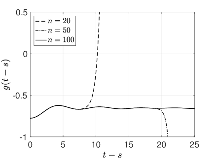
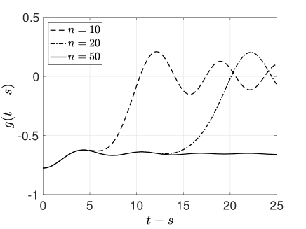
Figure 2: Dyson and Faber expansions of the Mori-Zwanzig memory kernel $g(t-s)$ in equation (97). Shown are results for different polynomial orders $n$. It is seen that the MZ-Faber series converges faster that the MZ-Dyson series.

In Figure 3 we study the accuracy of the MZ-Dyson and the MZ-Faber expansions in representing the mean wave solution as a function of the polynomial order $n$. To this end, we solve (96) numerically a linear multi-step (explicit) time integration scheme (3rd-order Adams-Bashforth) combined with a trapezoidal rule to discretize the memory integral. As easily seen, that the MZ-Faber expansion converges faster than the MZ-Dyson expansion.

Mean Wave Amplitude at $(r,\theta)=(1.1,0.1)$

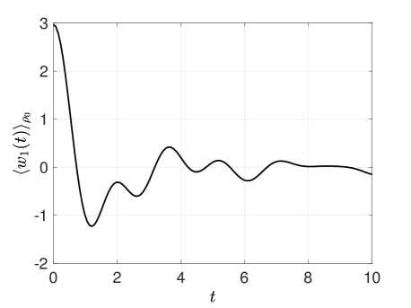
     MZ-Dyson Error                                               MZ-Faber Error

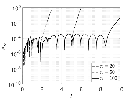
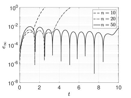
Figure 3: MZ-Dyson and MZ-Faber approximation errors of the mean wave amplitude at $(r,\theta)=(1.1,0.1)$ as a function of the polynomial order $n$. It is seen that the MZ-Faber expansion converges faster than the MZ-Dyson series.

5.2 Harmonic Chains on the Bethe Lattice

Dynamics of harmonic chains on Bethe lattices is a simple but illustrative Hamiltonian dynamical system that has been widely studied in statistical mechanics, mostly in relation to Brownian motion [2, 17, 15, 18, 26]. A Bethe lattice is a connected cycle-free graph in which each node interacts only with its neighbors. The number of such neighbors, is a constant of the graph called coordination number. This means that each node in the graph (with the exception of the leaf nodes) has the same number of edges connecting it to its neighbors. In Figure 4 we show two Bethe lattices with coordination numbers $l=2$ and $l=3$, respectively.

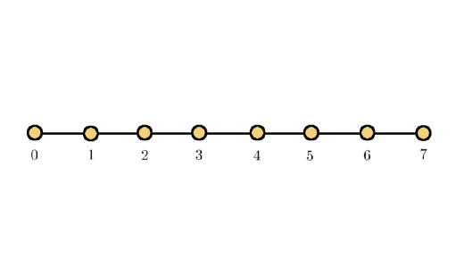
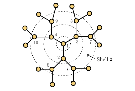
Figure 4: Bethe lattices with coordination numbers $2$ (left), and $3$ (right).

The Bethe graph is hierarchical and therefore it can be organized into shells, emanating from an arbitrary node. The number of nodes in the $k$-th shell is given by $N_{k}=l(l-1)^{k-1}$,while the total number of nodes within $S$ shells is

$$N=1+\sum_{k=1}^{S}N_{k}.$$ (99)

Next, we consider a coupled system of $N$ harmonic oscillators whose mutual interactions are defined by the adjacency matrix $\bm{B}^{(l)}$ of a Bethe graph with coordination number $l$ [4]. The Hamiltonian of such system can be written as

$$H(\bm{p},\bm{q})=\frac{1}{2m}\sum_{i=1}^{N}p_{i}^{2}+\frac{k}{2l}\sum_{i,j=1}^{N}B^{(l)}_{ij}(q_{i}-q_{j})^{2},$$ (100)

where $q_{i}$ and $p_{i}$ are, respectively, the displacement and momentum of the $i-$th particle, $m$ is the mass of the particles (assumed constant throughout the network), and $k$ is the elasticity constant that modulates the intensity of the quadratic interactions. We emphasize that the harmonic chain we consider here is one-dimensional. The Bethe graph basically just sets the interaction among the different oscillators. The dynamics of the harmonic chain on the Bethe lattice is governed by the Hamilton’s equations

$$\frac{dq_{i}}{dt}=\frac{\partial H}{\partial p_{i}},\qquad\frac{dp_{i}}{dt}=-\frac{\partial H}{\partial q_{i}}.$$ (101)

These equations can be written in a matrix-vector form as

$$\left[\begin{matrix}\dot{\bm{p}}\\ \dot{\bm{q}}\end{matrix}\right]=\left[\begin{matrix}\bm{0}&k\bm{B}^{(l)}-k\bm{D}^{(l)}\\ \bm{I}/m&\bm{0}\end{matrix}\right]\left[\begin{matrix}\bm{p}\\ \bm{q}\end{matrix}\right]=\bm{C}\left[\begin{matrix}\bm{p}\\ \bm{q}\end{matrix}\right],$$ (102)

where $\bm{B}^{(l)}$ is the adjacency matrix of the graph and $\bm{D}^{(l)}$ is the degree matrix. Note that (102) is a linear dynamical system. The time evolution of any phase space function $u(\bm{q},\bm{p})$ (quantity of interest) satisfies

$$\frac{du}{dt}= \{u,H\},$$

where

$$\{u,H\}=\sum_{i=1}^{N}\left(\frac{\partial u}{\partial q_{i}}\frac{\partial H}{\partial p_{i}}-\frac{\partial H}{\partial q_{i}}\frac{\partial u}{\partial p_{i}}\right)$$ (103)

denotes the Poisson Bracket. A particular phase space function we consider hereafter is the velocity auto-correlation function of a tagged oscillator, say the one at location $j=1$ (see Figure 4). Such correlation function is defined as

$$C_{p_{1}}(t)=\frac{\langle p_{1}(t)p_{1}(0)\rangle_{eq}}{\langle p_{1}(0)p_{1}(0)\rangle_{eq}},$$ (104)

where the average is an integral over the Gibbs canonical distribution (14).

5.2.1 Analytical Expressions for the Velocity Autocorrelation Function

The simple structure of harmonic chains on the Bethe lattice allows us to determine analytical expressions for the velocity autocorrelation function (104), e.g., [2, 26, 17].

Bethe Lattice with Coordination Number 2

Let us set $l=2$. In this case, the Bethe lattice is a a path graph, i.e., a one-dimensional chain of harmonic oscillators where each oscillator interacts only with the one at the left and at the right. We set fixed boundary conditions at the endpoint of the chain, i.e., $q_{0}(t)=q_{N+1}(t)=0$ and $p_{0}(t)=p_{N+1}(t)=0$ (particles are numbered from left to right). In this setting, the velocity auto-correlation function of the particle labeled with $j=1$ can be obtained analytically by employing Lee’s continued fraction method [17]. This yields the well-known $J_{0}-J_{4}$ solution

$$C_{p_{1}}(t)=J_{0}(2\omega t)-J_{4}(2\omega t),$$ (105)

where $J_{i}(t)$ is the $i$-th Bessel function of the first kind, and $\omega=k/m$. Here we choose $k=m=1$. The Hamilton’s equations (102) for the inner oscillators take the form

$$\left[\begin{matrix}\dot{\bm{p}}\\ \dot{\bm{q}}\end{matrix}\right]=\left[\begin{matrix}\bm{0}&\bm{B}^{(2)}-\bm{D}^{(2)}\\ \bm{I}&\bm{0}\end{matrix}\right]\left[\begin{matrix}\bm{p}\\ \bm{q}\end{matrix}\right],$$ (106)

where $\bm{B}^{(2)}$ and $\bm{D}^{(2)}$ are the adjacency matrix and the degree matrix of the Bethe lattice with $l=2$ (see Figure 4). As an example, if we consider five oscillators then $\bm{B}^{(2)}$ and $\bm{D}^{(2)}$ are given by

$$\bm{B}^{(2)}=\left[\begin{array}[]{ccc}0&1&0\\ 1&0&1\\ 0&1&0\end{array}\right],\qquad\bm{D}^{(2)}=\left[\begin{array}[]{ccc}2&0&0\\ 0&2&0\\ 0&0&2\end{array}\right].$$ (107)

Bethe lattice with $l=2$                                    Bethe lattice with $l=3$

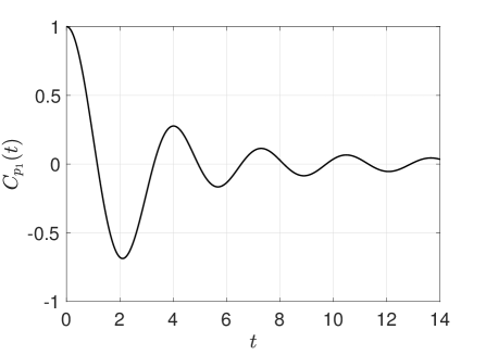
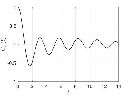
Figure 5: Velocity auto-correlation functions (105) (left) and (108) (right) of a tagged oscillator in an harmonic chain interacting on a Bethe lattice with coordination number $l=2$ and $l=3$, respectively.

Bethe Lattice with Coordination Number 3

Bethe graphs with $l=3$ can be represented as planar graphs (see Figure 4). The velocity auto-correlation function at the center node can be expressed analytically [26], in the limit of an infinite number of oscillators ($N\rightarrow\infty$), as

$$C_{p_{1}}(t) =\sum_{n=-\infty}^{+\infty}[G_{n}(t)+H_{n}(t)]J_{2n}(bt)$$ (108)

where

$$G_{n}(l) =\sum_{k=0}^{\infty}\frac{g_{k}(l)}{b^{2k-2}}\frac{1}{2\pi}\int_{a}^{\pi/2}d\theta\frac{\cos^{2}(\theta)}{\sin^{2k}(\theta)}\cos(2n\theta),\quad g_{k}(l)=-\sum_{j=k}^{\infty}\frac{(2j-1)!!}{[2^{j}(2j-1)j!]}a^{2j}c^{2(k-j)},$$

$$H_{n}(l) =\sum_{k=0}^{\infty}\frac{h_{k}(l)}{b^{-2k-2}}\frac{1}{2\pi}\int_{a}^{\pi/2}d\theta\frac{\cos^{2}(\theta)}{\sin^{-2k}(\theta)}\cos(2n\theta),\quad h_{k}(l)=-\sum_{j=k}^{\infty}\frac{(2j-1)!!}{[2^{j}(2j-1)j!]}a^{2(j-k)}c^{-2j}$$

and $a=\sqrt{2}-1$, $b=\sqrt{2}+1$ and $c=\sqrt{6}$. The Hamilton’s equations of motion in this case are ($k=m=1$)

$$\left[\begin{matrix}\dot{\bm{p}}\\ \dot{\bm{q}}\end{matrix}\right]=\left[\begin{matrix}\bm{0}&\bm{B}^{(3)}-\bm{D}^{(3)}\\ \bm{I}&\bm{0}\end{matrix}\right]\left[\begin{matrix}\bm{p}\\ \bm{q}\end{matrix}\right].$$ (109)

where $\bm{B}^{(3)},\bm{D}^{(3)}$ are the adjacency matrix and the degree matrix of the Bethe lattice with $l=3$ (see Figure 4). For example, if we label the oscillators as in Figure 4, and assume that the Bethe lattice has only three shells, i.e., $10$ oscillators ($4$ inner nodes, and $6$ leaf nodes) then the adjacency matrix and the degree matrix are

$$\bm{B}^{(3)}=\left[\begin{array}[]{cccccccccc}0&1&1&1&0&0&0&0&0&0\\ 1&0&0&0&1&1&0&0&0&0\\ 1&0&0&0&0&0&1&1&0&0\\ 1&0&0&0&0&0&0&0&1&1\\ 0&1&0&0&0&0&0&0&0&0\\ 0&1&0&0&0&0&0&0&0&0\\ 0&0&1&0&0&0&0&0&0&0\\ 0&0&1&0&0&0&0&0&0&0\\ 0&0&0&1&0&0&0&0&0&0\\ 0&0&0&1&0&0&0&0&0&0\end{array}\right],\qquad\bm{D}^{(3)}=\left[\begin{array}[]{cccccccccc}3&0&0&0&0&0&0&0&0&0\\ 0&3&0&0&0&0&0&0&0&0\\ 0&0&3&0&0&0&0&0&0&0\\ 0&0&0&3&0&0&0&0&0&0\\ 0&0&0&0&1&0&0&0&0&0\\ 0&0&0&0&0&1&0&0&0&0\\ 0&0&0&0&0&0&1&0&0&0\\ 0&0&0&0&0&0&0&1&0&0\\ 0&0&0&0&0&0&0&0&1&0\\ 0&0&0&0&0&0&0&0&0&1\end{array}\right].$$ (110)

5.2.2 Generalied Langevin Equation for the Velocity Autocorrelation Function

The evolution equation for the velocity autocorrelation function (104) was obtained in Section 3.4.2 and it is hereafter rewritten for convenience

$$\frac{dC_{p_{1}}(t)}{dt}=aC_{p_{1}}(t)+\int_{0}^{t}g(t-s)C_{p_{1}}(s)ds.$$ (111)

The initial condition is $C_{p_{i}}(0)=1$. The MZ-Dyson and MZ-Faber series expansions of the the memory kernel $g(t-s)$ are given by

$$g(t-s)=\sum_{j=0}^{n}\frac{g^{D}_{j}}{j!}(t-s)^{j},\qquad g(t-s)=\sum_{j=0}^{n}g^{F}_{j}e^{tc_{0}}\frac{J_{j}(2t\sqrt{-c_{1}})}{(\sqrt{-c_{1}})^{j}}$$

where

$$g_{j}^{D}=\bm{b}^{T}(\bm{M}_{11}^{T})^{j}\bm{a},\quad g_{j}^{F}=\bm{b}^{T}\mathcal{F}_{j}\left(\bm{M}_{11}^{T}\right)\bm{a}.$$

The definition of the matrix $\bm{M}_{11}^{T}$ and the vectors $\bm{a}$, $\bm{b}$ is the same as before. Here we used the fact that for any quadratic Hamiltonian we have $\left<p_{i}(0),q_{i}(0)\right>_{eq}=0$ and $\left<p_{i}(0),p_{j}(0)\right>_{eq}=\delta_{ij}$. In Figure 6 we study convergence of the MZ-Dyson and the MZ-Faber series expansion of the memory kernel in equation (46). As before, the MZ-Faber series converges faster that the MZ-Dyson series.

     MZ-Dyson                                                        MZ-Faber

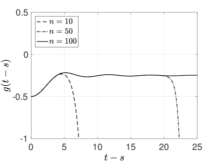
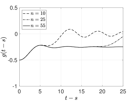
Figure 6: Harmonic chains of oscillators. Dyson and Faber expansions of the Mori-Zwanzig memory kernel $g(t-s)$. Shown are results for different polynomial orders $n$. It is seen that the MZ-Faber series converges faster that the MZ-Dyson series.

In Figure 7 and Figure 8, we study the accuracy of the MZ-Dyson and the MZ-Faber expansions in representing the velocity auto-correlation functions (105) and (108) (see Figure 5). Specifically, in these simulations we considered a chain of $N=100$ oscillators for the case $l=2$, and $8$ shells of oscillators for the case $l=3$, i.e., a total number of $N=766$ oscillators. The results in Figure 7 and Figure 8 show that both the MZ-Dyson and the MZ-Faber expansions of the memory integral yield accurate approximations of the velocity autocorrelation function, and that convergence is uniform with the polynomial order.

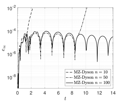
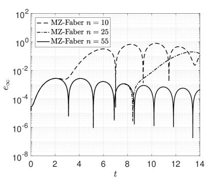
Figure 7: Accuracy of the MZ-Dyson and MZ-Faber expansions in representing the velocity auto-correlation function of the tagged oscillator $j=2$ in an harmonic chain interacting on the Bethe lattice with coordination number $2$. It is seen that the MZ-Dyson and the MZ-Faber expansions yield accurate predictions as we increase the polynomial order $n$. Moreover, the MZ-Faber expansion converges faster than the MZ-Dyson expansion.

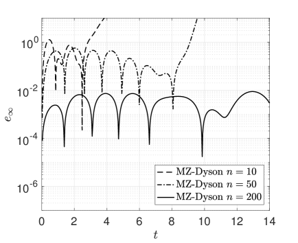
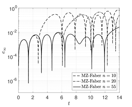
Figure 8: Accuracy of the MZ-Dyson and MZ-Faber expansions in representing the velocity auto-correlation function of the oscillator at the center of a Bethe lattice with coordination number $3$, $8$ shells and $N=766$ oscillators. It is seen that the MZ-Dyson and the MZ-Faber expansion yield accurate predictions as we increase the polynomial order $n$. Moreover, the MZ-Faber expansion converges faster than the MZ-Dyson series.

We emphasize that the new expansion of the MZ memory integral we developed can be employed to calculate phase space functions of harmonic oscillators on graphs with arbitrary topological structure. The following example shows the effectiveness of the proposed technique in calculating the velocity auto-correlation function of a tagged oscillator in a network sampled from the Erdös–Rényi random graph.

5.2.3 Harmonic Chains on Graphs with Arbitrary Topology

In this section we consider an harmonic chain on a graph with arbitrary topology. The Hamiltonian function is

$$H=\frac{1}{2m}\sum_{i=1}^{N}p_{i}^{2}+\frac{k}{2}\sum_{\begin{subarray}{c}i,j=1\\ i<j\end{subarray}}^{N}J_{ij}(q_{i}-q_{j})^{2},$$ (112)

where $J_{ij}$ is here is assumed is to be a sample from the Erdös–Rényi random adjacency matrix [5, 36]. In Figure 9 we study the accuracy of the MZ-Dyson and MZ-Faber expansions in approximating the velocity auto-correlation function of a tagged oscillator. In this case, no analytical solution is available and therefore we compared our solution to an accurate Monte Carlo benchmark. The lack of symmetry in each realization of the random network makes the velocity auto-correlation function dependent on the particular oscillator we consider.

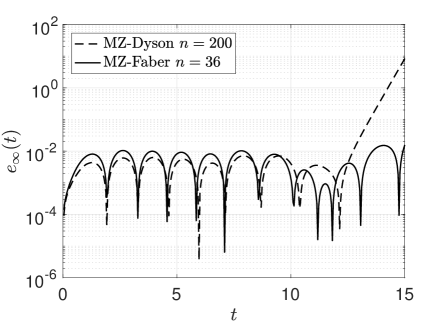
Figure 9: Aaccuracy of the MZ-Dyson and MZ-Faber expansions in approximating the velocity auto-correlation function of one tagged oscillator on a network obtained by sampling the Erdös-Rényi graph $G(100,0.1)$. The benchmark solution is computed by Monte Carlo simulation.

Acknowledgements

This work was supported by the Air Force Office of Scientific Research (AFOSR) grant FA9550-16-586-1-0092.

Appendix A Faber Polynomials

In this appendix we briefly review the theory of Faber polynomials in the complex plane. Such polynomial were introduced by Faber in [16] (see [46] for a through review), and they play an important role in theory of univalent functions and in the approximation of matrix functions [33, 37]. To introduce Faber polynomials, let

$$M=\left\{\Omega\subset\mathbb{C}:\,\textrm{$\Omega\neq\{\emptyset\}$ is compact and $\mathbb{C}\setminus\Omega$ is simply connected}\right\},$$

Given any set $\Omega\subset M$, by the Riemann mapping theorem there exits a conformal surjection

$$\psi:\hat{\mathbb{C}}\setminus\{w:|w|\leq\gamma\}\rightarrow\hat{\mathbb{C}}\setminus\Omega,\quad\psi(\infty)=\infty,\quad\psi^{\prime}(\infty)=1,$$ (113)

where $\hat{\mathbb{C}}$ is the Riemann sphere. The constant $\gamma$ is called capacity of $\Omega$. The $j-$th order Faber polynomial $\mathcal{F}_{j}(z)$ is defined to be the regular part of the Laurent expansion of $[\psi^{-1}(z)]^{j}$ at infinity, i.e.,

$$\mathcal{F}_{j}(z):=z^{j}+\sum_{k=0}^{j-1}\beta_{j,k}z^{k},\quad j\geq 0.$$ (114)

Let $\Gamma$ be the boundary of $\Omega$. For $R\geq\gamma$ we define the equipotential curve $\Gamma(R)$ as

$$\Gamma(R):=\{z:\psi^{-1}(z)=R\}.$$ (115)

We also denote as $\Omega(R)$ the closure of the interior of $\Gamma(R)$. Obviously, if $R=\gamma$ then we have $\Omega(R)=\Omega$ and $\Gamma(R)=R$. Any analytic function $f(z)$ on $\Omega$ can be uniquely expanded in terms of Faber polynomials as

$$f(z)=\lim_{m\rightarrow\infty}f_{m}(z)\qquad f_{m}(z)=\sum_{j=0}^{m}a_{j}(f)\mathcal{F}_{j}(z),$$ (116)

where the coefficients $a_{j}(f)$ are given be the complex integral

$$a_{j}(f)=\frac{1}{2\pi i}\int_{|w|=R}\frac{f\left(\psi(w)\right)}{w^{j+1}}dw.$$ (117)

It can be shown that $\mathcal{F}_{j}(z)$ satisfy the following recurrence relation

$$\mathcal{F}_{0}(z) =1,$$

$$\mathcal{F}_{1}(z) =z-c_{0},$$

$$\vdots$$

$$\mathcal{F}_{j}(z) =(z-c_{0})\mathcal{F}_{j-1}(z)-(c_{1}\mathcal{F}_{j-2}(z)+...+c_{j-1}\mathcal{F}_{0}(z))-(j-1)c_{j-1},\quad j\geq 2,$$ (118)

where $c_{0},c_{1},...$ are the coefficients of the Laurent series expansion of the mapping $\psi$, i.e.,

$$\psi(w)=w+c_{0}+\frac{c_{1}}{w}+\frac{c_{2}}{w^{2}}+\cdots,\qquad|w|>\gamma$$ (119)

From a computational viewpoint, it is convenient to limit the number of terms in the expansion (119). In this way, we can simplify the recurrence relation (A), the calculation of (117) and therefore significantly speed up computations. In this paper we consider the map

$$\psi(w)=w+c_{0}+\frac{c_{1}}{w},$$ (120)

which transforms circles into ellipses. In this case, the coefficients (117) can be obtained analytically by computing the integral

$$a_{j}(t) =\frac{1}{2\pi i}\int_{|w|=R}\frac{\exp\{t(w+c_{0}+c_{1}/w)\}}{w^{j+1}}dw,$$

$$=\frac{1}{(\sqrt{-c_{1}})^{j}}e^{tc_{0}}J_{j}(2t\sqrt{-c_{1}}),$$ (121)

where $J_{j}(x)$ is the Bessel function of the first kind. The number of terms in the Laurent series expansion (119) should be selected so that the spectrum of the operator $\mathcal{Q}\mathcal{L}$ lies entirely within the equipotential curve (115). In the numerical examples we discuss in Section 5 such spectrum turns out to be relatively concentrated around the imaginary axis. Hence, the second-order truncation (120), which defines an elliptical equipotential curve, guarantees fast convergence of the Faber series expansion of the orthogonal dynamics propagator.

Appendix B Faber Expansion of the Orthogonal Dynamics Propagator

Given any matrix representation of the operator $\mathcal{Q}\mathcal{L}$ (generator of the orthogonal dynamics) and a vector $v$, it is known that the sequence $f_{m}(\mathcal{Q}\mathcal{L})v$ (see equation (116)) converges to $f(\mathcal{Q}\mathcal{L})v$ for any analytic function $f(z)$ defined on $\Omega$, provided the spectrum of $\mathcal{Q}\mathcal{L}$ is in $\Omega$ (see [33]). Moreover, by the properties of Faber polynomials, it is known that the sequence $f_{m}(\mathcal{Q}\mathcal{L})$ approximates asymptotically $f(\mathcal{Q}\mathcal{L})$ on $\Omega$, as well as the sequence of best uniform approximation polynomials. In this sense, $f_{m}(\mathcal{Q}\mathcal{L})$ is said to be asymptotically optimal [13]. In particular, if we consider the exponential function $f(z)=e^{tz}$ and the conformal map (120), this yields the following $m$-th order Faber approximation of the orthogonal dynamics semigroup

$$e^{t\mathcal{Q}\mathcal{L}}\simeq\sum_{j=0}^{m}\frac{1}{(-c_{1})^{j/2}}e^{tc_{0}}J_{j}(2t\sqrt{-c_{1}})\mathcal{F}_{j}(\mathcal{Q}\mathcal{L}).$$ (122)

References

- [1] B. J. Alder and T. E. Wainwright. Decay of the velocity autocorrelation function. Phys. Rev. A, 1(1):18, 1970.
- [2] R. J. Baxter. Exactly solved models in statistical mechanics. Elsevier, 2016.
- [3] B. J. Berne. Projection operator techniques in the theory of fluctuations. In B. J. Berne, editor, Modern Theoretical Chemistry, pages 233–257. Plenum, New York, 1977.
- [4] N. Biggs. Algebraic graph theory, 1993.
- [5] B. Bollobás. Random Graphs. Cambridge University Press, 2001.
- [6] S. Chaturvedi and F. Shibata. Time-convolutionless projection operator formalism for elimination of fast variables. Applications to Brownian motion. Z. Phys. B, 35:297–308, 1979.
- [7] A. Chertock, D. Gottlieb, and A. Solomonoff. Modified optimal prediction and its application to a particle-method problem. J. Sci. Comput., 37(2):189–201, 2008.
- [8] A. J. Chorin, O. H. Hald, and R. Kupferman. Optimal prediction and the Mori-Zwanzig representation of irreversible processes. Proc. Natl. Acad. Sci. USA, 97(7):2968–2973, 2000.
- [9] A. J. Chorin, R. Kupferman, and D. Levy. Optimal prediction for Hamiltonian partial differential equations. J. of Comput. Phys., 162(1):267–297, 2000.
- [10] A. J. Chorin and P. Stinis. Problem reduction, renormalization and memory. Comm. App. Math. and Comp. Sci., 1(1):1–27, 2006.
- [11] R. Dautray and J.-L. Lions. Mathematical Analysis and Numerical Methods for Science and Technology: Vol. 3 Spectral Theory and Applications. Springer Science & Business Media, 2012.
- [12] J. Dominy and D. Venturi. Duality and conditional expectation in the Nakajima-Mori-Zwanzig formulation. J. Math. Phys., 58:082701, 2017.
- [13] M. Eiermann. On semi-iterative methods generated by Faber polynomials. 56:139–156, 1989.
- [14] K.-J. Engel and R. Nagel. One-parameter semigroups for linear evolution equations, volume 194. Springer, 1999.
- [15] P. Español. Dissipative particle dynamics for a harmonic chain: A first-principles derivation. Phys. Rev. E, 53(2):1572, 1996.
- [16] G. Faber. Über polynomische entwickelunge. Mathematische Annalen, 57:389–408, 1903.
- [17] J. Florencio, , and H. M. Lee. Exact time evolution of a classical harmonic-oscillator chain. Phys. Rev. A, 31(5):3231, 1985.
- [18] G. W. Ford, M. Kac, and P. Mazur. Statistical mechanics of assemblies of coupled oscillators. J. Math. Phys., 6(4):504–515, 1965.
- [19] R. F. Fox. Functional-calculus approach to stochastic differential equations. Phys. Rev. A, 33(1):467–476, 1986.
- [20] A. Gouasmi, E. J. Parish, and K. Duraisamy. A priori estimation of memory effects in reduced-order models of nonlinear systems using the Mori–Zwanzig formalism. Proc. R. Soc. A, 473:1–24, 2017.
- [21] G. D. Harp and B. J. Berne. Time-correlation functions, memory functions, and molecular dynamics. Phys. Rev. A, 2(3):975, 1970.
- [22] J. S. Hesthaven, S. Gottlieb, and D. Gottlieb. Spectral methods for time-dependent problems. Cambridge Univ. Press, 2007.
- [23] N. G. Van Kampen and I. Oppenheim. Brownian motion as a problem of eliminating fast variables. Physica A: Stat. Mech. and Appl., 138(1-2):231–248, 1986.
- [24] T. Karasudani, K. Nagano, H. Okamoto, and H. Mori. A new continued-fraction representation of the time-correlation functions of transport fluxes. Progress of Theoretical Physics, 61(3):850–863, 1982.
- [25] T. Kato. Perturbation theory for linear operators. Springer-Verlag, fourth edition, 1995.
- [26] J. Kim and I. Sawada. Dynamics of a harmonic oscillator on the Bethe lattice. Phys. Rev. E, 61(3):R2172, 2000.
- [27] B. O. Koopman. Hamiltonian systems and transformation in Hilbert spaces. Proc. Natl. Acad. Sci. USA, 17(5):315–318, 1931.
- [28] H. M. Lee. Solutions of the generalized langevin equation by a method of recurrence relations. Phys. Rev. B, 26(5):2547, 1982.
- [29] H. M. Lee. Derivation of the generalized Langevin equation by a method of recurrence relations. J. Math. Phys., 24:2512–2514, 1983.
- [30] Huan Lei, N. A. Baker, and X. Li. Data-driven parameterization of the generalized Langevin equation. PNAS, 113(50):14183–14188, 2016.
- [31] C. Moler and C. Van Loan. Nineteen dubious ways to compute the exponential of a matrix. SIAM review, 20(4):801–836, 1978.
- [32] C. Moler and C. Van Loan. Nineteen dubious ways to compute the exponential of a matrix, twenty-five years later. SIAM review, 45(1):3–49, 2003.
- [33] I. Moret and P. Novati. The computation of functions of matrices by truncated faber series. 22(5-6):697–719, 2001.
- [34] H. Mori. A continued-fraction representation of the time-correlation functions. Progress of Theoretical Physics, 34(3):399–416, 1965.
- [35] F. Moss and P. V. E. McClintock, editors. Noise in nonlinear dynamical systems. Volume 1: theory of continuous Fokker-Planck systems. Cambridge Univ. Press, 1995.
- [36] M. E. J. Newman, S. H. Strogatz, and D. J. Watts. Random graphs with arbitrary degree distributions and their applications. Phys. Rev. E, 64:026118, 2001.
- [37] P Novati. Solving linear initial value problems by Faber polynomials. Numerical linear algebra with applications, 10(3):247–270, 2003.
- [38] E. J. Parish and K. Duraisamy. Non-Markovian closure models for large eddy simulations using the Mori-Zwanzig formalism. Phys. Rev. Fluids, 2:014604, 2017.
- [39] K. S. Singwi, , and A. Sjölander. Theory of atomic motions in simple classical liquids. Phys. Rev., 167(1):152, 1968.
- [40] L. Sjogren. Numerical results on the velocity correlation function in liquid argon and rubidium. Journal of Physics C: Solid State Physics, 13(5):705, 1980.
- [41] L. Sjogren and A. Sjolander. Kinetic theory of self-motion in monatomic liquids. Journal of Physics C: Solid State Physics, 12(21):4369, 1979.
- [42] I. Snook. The Langevin and generalised Langevin approach to the dynamics of atomic, polymeric and colloidal systems. Elsevier, first edition, 2007.
- [43] P. Stinis. A comparative study of two stochastic model reduction methods. Physica D, 213:197–213, 2006.
- [44] P. Stinis. Higher order Mori-Zwanzig models for the Euler equations. Multiscale Modeling & Simulation, 6(3):741–760, 2007.
- [45] P. Stinis. Renormalized Mori–Zwanzig-reduced models for systems without scale separation. Proc. R. Soc. A, 471(2176):20140446, 2015.
- [46] P. K. Suetin and E. V. Pankratiev. Series of Faber polynomials. CRC Press, 1998.
- [47] U. Umegaki. Conditional expectation in an operator algebra I. Tohoku Math. J., 6(2):177–181, 1954.
- [48] D. Venturi, H. Cho, and G. E. Karniadakis. The Mori-Zwanzig approach to uncertainty quantification. In R. Ghanem, D. Higdon, and H. Owhadi, editors, Handbook of uncertainty quantification. Springer, 2016.
- [49] D. Venturi and G. E. Karniadakis. Convolutionless Nakajima-Zwanzig equations for stochastic analysis in nonlinear dynamical systems. Proc. R. Soc. A, 470(2166):1–20, 2014.
- [50] R. O. Watts and I. K. Snook. Perturbation theories in non-equilibrium statistical mechanics II. Methods based on memory function formalism. Molecular Physics, 33(2):443–452, 1977.
- [51] Y. Zhu, J. M. Dominy, and D. Venturi. Rigorous error estimates for the memory integral in the Mori-Zwanzig formulation. arXiv, (1708.02235):1–32, 2017.
- [52] R. Zwanzig. Nonequilibrium statistical mechanics. Oxford University Press, 2001.