Localization enhanced and degraded topological-order in interacting p-wave wires

Abstract

We numerically study the effect of disorder on the stability of the many body zero mode in a Kitaev chain with local interactions. Our numerical procedure allows us to resolve the position-space and multi-particle structure of the zero modes, as well as providing estimates for the mean energy splitting between pairs of states of opposite fermion parity, over the full many body spectrum. We find that the parameter space of a clean system can be divided into regions where interaction induced decay transitions are suppressed (Region I) and where they are not (Region II). In Region I we observe that disorder has an adverse effect on the zero mode, which extends further into the bulk and is accompanied by an increased energy splitting between pairs of states of opposite parity. Conversely Region II sees a more intricate effect of disorder, showing an enhancement of localization at the system’s end accompanied by a reduction in the mean pairwise energy splitting. We discuss our results in the context of the Many-Body Localization (MBL). We show that while the mechanism that drives the MBL transition also contributes to the fock-space localization of the many-body zero modes, measures that characterize the degree of MBL do not necessarily correlate with an enhancement of the zero-mode or an improved stability of the topological region.

The prospects of building quantum devices using topological superconductors has caused a great deal of excitement. In these systems, emergent excitations known as Majorana zero modes that occur at sample edges obey non-Abelian exchange statistics Read2000 ; Ivanov2001 ; Kitaev2001 ; Kitaev2006 ; Nayak2008 , and their manipulation is inherently protected from common sources of decoherence. This potentially revolutionary feature has spurred a great deal of theoretical Fu2008 ; Lutchyn2010 ; Oreg2010 ; Duckheim2011 ; Chung2011 ; Choy2011 ; Kjaergaard2012 ; Martin2012 ; NadjPerge2013 and experimental work Mourik2012 ; Deng2012 ; Das2012 ; Finck2013 ; Churchill2013 ; Albrecht2016 ; Zhang2016 ; Deng2016 ; NadjPerge2014 ; Ruby2015 ; Pawlak2016 .

The experimental observations in proximity coupled systems are typically well described within a quasi-particle framework (see e.g Motrunich2001 ; Brouwer2011 ; Brouwer2011b ; Akhmerov2011 ; Rieder2012 ; Rieder2013 ; DeGottardi2013 ; Pientka2013 ; Stoudenmire2011 ; Lutchyn2011 ; Sela2011 ; Lobos2012 ; Crepin2014 ; Hassler2012 ; Thomale2013 ; Katsura2015 ; Gergs2016 ; Gangadharaiah2011 ), suggesting that at temperatures well below the gap, the properties of these systems are stable to imperfect conditions such as electron-electron interactions. Recently there have been efforts to understand the stability of these non-abelian excitations at energies and temperatures well above the topological gap Gangadharaiah2011 ; Goldstein2012 ; Fendley2016 ; Miao2017 ; McGinely2017 ; Kells2015a ; Kemp2017 ; Moran2017 ; Else2017 ; Fendley2012 ; Fendley2014 ; Jermyn2014 ; Moran2017 ; Kells2015b ; CommentStrongZeroMode ; CommentZn . These studies directly relate to the effectiveness of symmetry-protected-topological (SPT) systems as platforms for quantum memories.

In this respect an important recent idea connected to the phenomenon of many-body localization Gornyi2005 ; Basko2006 suggests that the stability of non-abelian excitations at high energies can be enhanced with additional protection due to disorder-induced localization Huse2013 ; Bauer2013 ; Chandran2014 ; Kjall2014 ; Carmele2015 ; Bahri2015 ; Wootton2011 ; Stark2011 ; Bravyi2012 ; Potter2016 . This notion has been called localization-protected topological-order LocTop and its consequences could be far-reaching, allowing for topological quantum processors that can be operated at high temperatures. Although this would be a remarkable feature, the precise way in which the interplay between disorder and interactions affect the topological order has proved difficult to pin down.

One complication is that both disorder and interactions are known to be universally detrimental to this symmetry-protected topological-phase. By gradually destroying the superconducting gap which protects it, potential disorder is known to make the Majorana zero modes less localized at the system’s boundary. This drives a topological phase transition at a critical strength when the mean free path is half the superconducting coherence length $l_{c}=\xi/2$Motrunich2001 ; Brouwer2011 ; Brouwer2011b ; Akhmerov2011 ; Rieder2012 ; Rieder2013 ; DeGottardi2013 ; Pientka2013 .

Interactions can similarly reduce the topological protection and drive a phase transition to a non-topological phase (see e.g. Gangadharaiah2011 ; Stoudenmire2011 ; Lutchyn2011 ; Sela2011 ; Lobos2012 ; Crepin2014 ; Gergs2016 ; Hassler2012 ; Thomale2013 ; Katsura2015 ). This can be understood in terms of two mechanisms that lift the topological degeneracy associated with the mode: (1) Local charging effects, which give rise to local potentials, can measure the occupation of the zero-mode and (2) Interaction induced decay transitions that change the occupancy of the zero-mode while exciting quasi-particle excitations. As both disorder and interactions reduce the topological protection, it is reasonable to think that they combine to destroy the topological phase even further. Indeed, analyses of both effects using abelian bosonization suggests that repulsive interactions and disorder do indeed reinforce their destructive effects on the topological phase Lobos2012 ; Crepin2014 .

These destructive effects add an additional level of complexity to an already difficult numerical problem. This is because in order to demonstrate some enhanced topological protection in the interacting system, one typically needs to obtain precise information about the full many body spectrum, using a statistically significant number of different disorder realisations. Although this full spectrum resolution can be in principle obtained using exact diagonalisation methods, the range of system sizes accessible to this technique is very limited. This, and the fact that the background negative effects of both interactions and disorder are also strongly present in small systems, makes extrapolation to larger more meaningful systems essentially impossible.

In this manuscript we address these questions from the perspective of many-body-zero-modes Gangadharaiah2011 ; Goldstein2012 ; Fendley2016 ; McGinely2017 ; Miao2017 ; Kells2015a ; Kemp2017 ; Moran2017 ; Else2017 ; Fendley2012 ; Fendley2014 ; Jermyn2014 ; Moran2017 ; Kells2015b ; CommentStrongZeroMode ; CommentZn . We focus on the simplest topological superconductor, the Kitaev chain, in the presence of short range interactions and potential disorder. We study these effects using exact diagonalisation and a numerical procedure that approximates the odd-parity multi-particle steady-states of the interacting commutator $\mathcal{H}=[H,\bullet]$ Kells2015b . In this respect we showcase a key improvement; namely its implementation using Matrix-Product-Operators (MPO) Crosswhite2008 and DMRG-like optimisation Schollwock2011 . This super-operator formalism allows us to resolve the position-space and multi-particle structure of the zero-modes as well as to extract statistical information about the entire many-body spectrum. Our analysis shows that, in weakly interacting topological superconductors, disorder can trigger separate effects that both enhance and degrade topological order. As the strength of each mechanism is dependent on the underlying parameter space, this allows for the identification of regimes of parameter space where disorder can degrade (Region I) or improve (Region II) the underlying topological protection of the zero mode.

The structure of the manuscript is as follows. In section I we review the Kitaev chain (or p-wave wire) model and qualify our central results using both band-projection and perturbation theory. In this section we also review the key results pertaining to MBL and their connection to so called many body zero modes. In section II we discuss our MPO numerical methodology and examine the connection between the structure of the zero-mode expansion and the statistical estimates of the pairwise energy level splitting. In section III we outline the numerical results themselves.

We also include several appendices: In Appendix A we discuss the perturbative case for zero-modes. In Appendix B we discuss our MPO algorithm and add more details to the error analysis provided in the main text. In Appendix C we provide the results from exact diagonalization calculations. In Appendix D we outline the formal construction of many-body zero modes and discuss the relationship between energy relaxation processes and resulting multi-particle structure of the zero-mode position space expansion.

I Model and physical picture

We formulate our results using the lattice p-wave superconducting model or Kitaev chain Kitaev2001 :

$$H_{0} = -\sum_{j=1}^{N}\mu_{j}(c_{j}^{\dagger}c_{j}-\frac{1}{2})-\sum_{j=1}^{N-1}tc_{j}^{\dagger}c_{j+1}+\Delta c_{j}^{\dagger}c_{j+1}^{\dagger}+{\rm h.c.}$$ (1)

where coefficients $t$, $\Delta$ and $\mu_{i}$ are for the hopping, pairing amplitude and local chemical potential at site $i$ respectively. To model disorder we allow the local chemical potential to vary around an average value $\mu$ with the standard deviation set by the parameter $\lambda$. The normal-state mean-free-path is given as $l=\frac{v_{F}^{2}}{\lambda^{2}}$, where $\hbar v_{F}=2ta\sqrt{\frac{\mu+2t}{t}}$ is the Fermi-velocity.

Interactions are included through the local quartic term

$$H_{I}=2U\sum_{j=1}^{N-1}\left(c_{j}^{\dagger}c_{j}-\frac{1}{2}\right)\left(c_{j+1}^{\dagger}c_{j+1}-\frac{1}{2}\right).$$ (2)

The phase of the p-wave superconducting pairing potential can be chosen to be real. When $|\Delta|>0$ and $|\mu|<2t$ the $H_{0}$ system is known to be in a topological phase with Majorana zero modes exponentially localised at each end of the wireKitaev2001 . In what follows it is useful to work in a basis of position space Majorana operators defined as:

$$\gamma_{2j-1}=i(c^{\dagger}_{j}-c_{j}^{\phantom{\dagger}}),\gamma_{2j}=(c^{\dagger}_{j}+c_{j}^{\phantom{\dagger}}).$$ (3)

These obey $\{\gamma_{i},\gamma_{j}\}=2\delta_{ij}$ and thus $\gamma_{i}=\gamma_{i}^{\dagger}$ and $\gamma_{i}^{2}=I$.

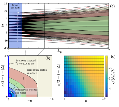
Figure 1: Figure (a) : the full many body spectrum of a small $L=12$ system with $\Delta=0.9t$ and $U=0$ . We label bands according to the number of bulk (non-zero mode) excitations above the ground state. When band crossing occur, interactions can induce avoided level crossings between bands with different fermion number and different occupation of the zero mode. These are generally different in even and odd sectors; causing the degeneracy associated with the zero mode to lift. Away from the flat band limit $\mu=0$ and $t=|\Delta|$, bands in the middle of the spectrum begin to cross. Interactions induced transitions require the excitation of a large number of quasi-particle excitations in this limit. Figure (b): phase diagram constructed by outlining where crossings first occur for a $L=50$ system. It also indicates a key exception along the $\mu=0$ line, where the crossings are protected by additional symmetry Fendley2016 . Figure (c): $\sqrt{\langle\mathcal{E}_{2}}\rangle/U$ given by (12) in the clean system with $U=0.1t$, calculated using the MPS/DMRG algorithm for a system of length $L=50$. Unless specified otherwise, all energy scales are in units of $t$.

When interactions are absent, the many body spectrum is doubly degenerate. The two states that form an almost degenerate pair differ by the occupation of the zero mode, made up of two Majorana bound states exponentially localized at the two ends of the chain. The energy splitting between pairs depends on the spatial decay rate of the Majorana zero modes and is given as $\delta\sim e^{-L/\xi}$ where $\xi\sim t/\Delta$ is the superconducting coherence length.

Interactions can lift the two fold degeneracy in two ways. Firstly, by introducing local charging effects, which can measure the occupation of the zero mode. As information of the occupancy of the zero mode is stored non-locally, this lifting occurs at an order of the interaction strength $U$ which scales with the system size $\sim U^{L}$. Crucially, interactions can also change the occupancy of the zero mode by introducing energy relaxation processes whereby a finite energy excitation can decay into the zero mode while exciting a pair of quasi-particles. These decay processes serve as a lifetime for non-interacting states, which can be estimated from a Fermi golden rule type analysis. The simplest lowest-order decay process is the transition of a quasi-particle excitation to two quasi-particle excitations, while changing the occupancy of the zero mode (leaving all other quasi-particle excitations unaltered):

$$\Gamma\sim\frac{|U|^{2}}{\Delta\epsilon}$$ (4)

where $\Delta\epsilon=2\epsilon^{0/1}_{min}-\epsilon^{1/0}_{max}$ where the superscript denote the state of the zero-mode, $2\epsilon^{0/1}_{min}$ is the minimal energy of a state with two bulk quasi-particle excitations and $\epsilon^{1/0}_{max}$ is the maximal energy of a state with a single bulk quasi-particle excitation.

Our main insight is then based on the fact that in a clean system there are regions of parameter space where these real decay transitions are suppressed, we refer to this regime, as Region I. In the clean non-interacting limit, Region I can be defined by the requirement that $\Gamma<\Delta\epsilon$ which can be written as: [see Appendix A for a detailed discussion]:

$$|\mu|<\frac{2t-U}{3},\quad\quad\quad\quad\quad\quad\text{if }|{\mu}|>\frac{2}{t}(t^{2}-\Delta^{2})$$ (5)

$$|\mu|<2|\Delta|\sqrt{4-\frac{\mu^{2}}{t^{2}-\Delta^{2}}}-2t-U,\text{otherwise}$$

The complement space, where $\Gamma>\Delta\epsilon$, is identified as Region II. We remark that while Region I can be prominent in lattice models, experimental realizations of the Kitaev chain are typically characterized by weak proximity coupling $\Delta\ll t$, and the parameter space is dominated by Region II.

Disorder modifies this picture in three ways by: (1) increasing the coherence length $\xi$, making the Majorana zero modes less localized at the systems boundary Motrunich2001 ; Brouwer2011 ; Brouwer2011b ; Akhmerov2011 ; Rieder2012 ; Rieder2013 ; DeGottardi2013 ; Pientka2013 , (2) broadening the width of the single particle excitation band and (3) decreasing the localisation length of bulk excitations Anderson58 .

On a single particle level, both Regions I and II experience a similar effect of disorder which extends the zero mode operator further into the bulk, thus gradually lifting the degeneracy that protects the topological phase. However, on top of this single particle effect, disorder plays a much more subtle role: In Region I disorder has a universally adverse effect because, by also broadening the bulk single particle excitation band, it also drives the system towards a regime where decay transitions can occur. Although disorder may also increase the number of decay transition in Region II, in this case the energy splitting associated with these decay transitions is reduced, as shown in Figure 2. This behaviour is directly connected to the spatial localization of the bulk states, which suppress these decay processes within a localization length (see e.g. Gornyi2005 ; Basko2006 ; Huse2013 ).

These competing behaviors are revealed in the numerical analysis (see section III) of the multi-particle structure where we see clear evidence of both localization-enhanced and localization-diminished topological-order. Near the system edges, in both Regions I and II, disorder increases the decay-length of single particle terms as well as locally clustered components. However, further from the sample edge, the spatial decay of the locally clustered components shows a clear distinction between the two regions of phase space, as highlighted in Fig. 4 (c) and (d). In Region I all local clusters extend further into the bulk in the presence of disorder. Conversely, Region II exhibits a transition from non-decaying local-clusters (see 7) in the clean system to exponentially decaying in a disordered medium.

We will also show how the aforementioned decay of local multi-particle clusters is reflected in the mean energy-level-splitting $\langle\delta\rangle$ between pairs of states from opposite parity sectors. Region I, which is dominated by the single particle behavior, exhibits predominantly localization-diminished topological order. Conversely, Region II displays localization-enhanced topological order at moderate disorder strength.

Figure 2: The probability distribution of the first-order interaction-induced decay-amplitude $|d|=|\langle n\,|H_{I}|\,m\rangle|$ decays as we increase the disorder strength $\lambda$. Here $|\,m\rangle$ is a non interacting state with two bulk excitations and the zero mode unoccupied and $|\,n\rangle$ is a non interacting state with a single bulk excitation and the zero mode occupied. The plots were obtained in Region II for $\mu=-t$, $\Delta=0.5t$, $U=0.1t$ and for a wire of length $L=100$ . Increasing the value of the disorder parameter $\lambda$ shifts the distribution towards zero splitting.

Relation to many body localization The observed enhancement of topological protection is related to, but distinct from, Many-Body-Localization (MBL) Gornyi2005 ; Basko2006 . In particular, while our analysis shows that disorder induces opposing effects on the zero mode structure in the two regimes of parameters, measures that characterise the extent of MBL show no prominent differences between the two regions. Nor do they demonstrate any noticeable change as the topological order is destroyed.

The transition to an MBL phase can be understood as a dynamical phase transition, in the sense that one can construct an extensive number of integrals of motion Huse2014 ; Chandran2015a ; Serbyn2013a that constrain the dynamics of the system to a degree that it does not thermalize in the way expected from the eigenstate thermalisation hypothesis (ETH)  Deutsch1991 ; Srednicki1994 ; Srednicki1996 . These features of the ETH-MBL transition give rise to a rich variety of signatures, which can be detected in the level statistics Bauer2013 ; Oganesyan2007 ; Pal2010 ; Cuevas2012 ; Laumann2014 ; Luitz2015 , in the entanglement entropy Bauer2013 ; Kjall2014 ; Grover2014 , in the response Berkelbach2010 ; BarLev2015 and in the dynamics of the system under consideration Znidaric2008 ; Bardarson2012 ; Serbyn2013 .

To address the possible association between enhanced topological order and the ETH-MBL transition we focus on one sensitive characterization of the transition that is based on the eigenvalues of the generalised single-particle density matrix

$$R_{n}=\left[\begin{array}[]{cc}\rho&\kappa\\ \kappa^{\dagger}&I-\rho\end{array}\right],$$ (6)

where $\rho_{ij}=\langle n\,|c_{i}^{\dagger}c_{j}|\,n\rangle$, $\kappa_{ij}=\langle n\,|c_{i}^{\dagger}c_{j}^{\dagger}|\,n\rangle$, and $|\,n\rangle$ is a many body eigenstate. Similarly to Ref. Bera2015, , for which the system was not superconducting and so $\rho$ was sufficient, the eigenvalues of $R_{n}$ constitute the occupation spectrum and this exhibits distinct behaviour in the two phases. In the delocalized (ETH) phase, they are expected to be close to the mean filling fraction, while in the localized phase (MBL) they should tend to their asymptotic values $\in\{0,1\}$. Consequently, it is possible to characterize the transition to an MBL phase by a step-like jump in the occupation spectrum.

In Fig. 3 we show the value of the discontinuous jump in the occupation spectrum of the single particle density matrix, in Region I (red curve) and Region II (black curve) for a system of size $L=15$. Although disorder induces opposing effects on the zero mode structure in the two regimes of parameters, this MBL measure does not distinguish between the two regions. Moreover it is also insensitive to the underlying topological order which, for the representative parameters for Regions I and II, is destroyed by disorder strength $\lambda\gtrapprox 2.9$ and $2.3$ respectively.

The distinction between localization and the observed enhancement of topological protection is twofold. Firstly, while localization in Fock space is known to suppress decay transitions, not all transitions are detrimental to the zero mode. Consequently, localisation induced protection can only occur in regions of phase space where these harmful decay process are abundant. This corresponds to our definition of Region II. As standard measures of localization cannot distinguish transitions that couple states with different occupation of the zero mode and those who do not, these cannot pick up the difference between the two regimes of parameter, as we show in Fig 3. Secondly, it is not clear that the topological superconducting phase survives strong potential disorder. That is to say, in the limit when the system breaks down into segments of localization length, topological protection can be lifted altogether due the small size of each segment as compared to the superconducting coherence length, which is known to increase in the presence of potential disorder. This single particle effect is crucial to the suppression of topological protection in topological superconductors, but plays no role in the localization transition. It is for this reason that calculations aimed at detecting the MBL transition (such as the one showed in Fig 3), are insensitive to the disorder induced topological phase transition.

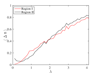
Figure 3: The dependence of the discontinuous jump of the occupations of natural orbitals, with increasing disorder strength $\lambda$ for Region I ($\Delta=0.7t$, $\mu=-0.2t$ and $U=0.1t$, red curve) and Region II ($\Delta=0.5t$, $\mu=-t$ and $U=0.1t$, black curve). Following Ref. Bera2015, , in the delocalized phase, the occupations are expected to be close to the mean filling fraction, while in the localized phase they tend to their asymptotic values $\langle n_{N}\rangle=\{0,1\}$, and the occupation spectrum exhibits a discontinuous jump $\Delta n=n_{L+1}-n_{L}$. Consequently, the averaged value of the discontinuous jump in the occupation spectrum can be used to characterize the ETH-MBL transition. While disorder is shown to induce opposing effects on the zero mode structure in the two regime of parameters, see Fig. 4, its effect on the occupation spectrum is essentially identical. The data shown is for a system of length $L=15$ and each data point in averaged over 100 disorder realisations with a sampling of 100 states per realisation (50 in each sector) around $E=0$.

II Numerical methods

We seek to identify an operator which:

1. Commutes with the Hamiltonian, up to small corrections: $[H,\Gamma]\sim 0$.

2. Anticommutes with the total parity: $\{P,\Gamma\}=0$.

3. Is Hermitian: $\Gamma=\Gamma^{\dagger}$.

4. Is its own inverse: $\Gamma^{2}=I$.

Our numerical procedure is based on giving matrix representations to the commutator $\mathcal{H}=[H,\bullet]$ using the operator (Hilbert-Schmidt) inner product Goldstein2012 ; Kells2015b . This procedure is based on what is called the Choi-Jamiolkowski-isomorphism Choi1972 ; Choi1975 ; Jamiolkowski1972 , also referred to as Third Quantization Prosen2008 . The numerical algorithm itself can be seen as a hybridization of the variational position-space algorithm applied in Ref. Kells2015b, , and methods that represent super-operators such as $\mathcal{H}$ (or more generally the Limblad super-operator) as Matrix-Product-Operators (see e.g. Mascarenhas2015 ; Cui2015 )

In the presence of interactions, this procedure produces a many body operator of the general form:

$$\Gamma=\sum_{i}^{2L}u^{(1)}(i)\gamma_{i}+\sum_{ijk}^{2L}u^{(3)}(i,j,k)\gamma_{i}\gamma_{j}\gamma_{k}+...$$ (7)

where $\gamma_{i}$ is a Majorana operator at position $i$ and $u^{(n)}(i,j,k,..)$ is the coefficient of the $n$ particle term, with $n$ majorana modes located at positions $i<j<k$. We numerically calculate the zero mode wave function by identifying the operators that minimize the expression $\operatorname{Tr}(\Gamma_{L/R}^{\dagger}\times[H,[H,\Gamma_{L/R}]])/2^{L}$, subject to constraints 2-3, and where $\Gamma_{L/R}$ stands for zero mode localized at the left/right side of the chain. Although constraint 4 is not actively enforced, our methodology insures that it is approximately obeyed.

Statistics of level splittings and error estimates: In addition to probing the local structure of the zero mode (7), the methodology described above allows us to estimate the average level splitting between pairs of states from different parity sectors. To see this we first examine the Hamiltonian in the system eigenbasis. In the topological phase the many body spectrum is doubly degenerate up to corrections $\delta_{n}$:

$$H =\sum_{n}E_{n}\left[|n_{1}\rangle\langle n_{1}|+|n_{0}\rangle\langle n_{0}|\right]$$

$$+\delta_{n}/2\left[|n_{1}\rangle\langle n_{1}|-|n_{0}\rangle\langle n_{0}|\right].$$ (8)

Here $0/1$ refers to the occupation of the zero-mode. In the non-interacting system, the zero-mode operators are eigenmodes of the Hamiltonian, $\left[|n_{0}\rangle\langle n_{1}|,H\right]=\delta\left(|n_{0}\rangle\langle n_{1}|\right)$, which means that the many body spectrum consists of pairs of states distinguished by the occupation of the zero mode, and displaced by a uniform energy splitting: $\delta_{n}=\delta\sim e^{-L/\xi}$. In general, however, interactions give rise to a distribution of pair splitting $P(\delta_{n})$ which are not necessarily exponentially small.

In this basis the MPS/MPO methodology constructs an approximate Majorana zero mode with the following structure

$$\Gamma_{L} =\sum_{n}(1-\alpha^{L}_{n})\left[|n_{0}\rangle\langle n_{1}|+|n_{1}\rangle\langle n_{0}|\right]$$ (9)

$$+\sum_{n\neq m}\beta^{L}_{nm}\left[|n_{0}\rangle\langle m_{1}|+|m_{1}\rangle\langle n_{0}|\right]$$

$$\Gamma_{R} =-i\sum_{n}(1-\alpha^{R}_{n})\left[|n_{0}\rangle\langle n_{1}|-|n_{1}\rangle\langle n_{0}|\right]$$ (10)

$$-i\sum_{n\neq m}\beta^{R}_{nm}\left[|n_{0}\rangle\langle m_{1}|-|m_{1}\rangle\langle n_{0}|\right]$$

where $\alpha$- and $\beta$-terms represent diagonal/off-diagonal errors respectively. The commutator of the near zero mode operators $\Gamma_{L/R}$ with the interacting Hamiltonian, allows to estimates the energy level statistics:

$$\mathcal{E}_{1} =i\operatorname{Tr}(\Gamma_{L}\times[H,\Gamma_{R}])/2^{L}=\langle\delta\rangle+\chi_{1}$$ (11)

$$\mathcal{E}_{2} =\operatorname{Tr}(\Gamma_{L}\times[H,[H,\Gamma_{L}]])/2^{L}=\langle\delta^{2}\rangle+\chi_{2}$$ (12)

where

$$\chi_{1} =-\frac{1}{2^{L}}\sum_{n}\delta_{n}\left[\alpha^{L}_{n}+\alpha^{R}_{n}-\alpha^{L}_{n}\alpha^{R}_{n}\right]$$ (13)

$$+\frac{1}{2^{L}}\sum_{n\neq m}\beta^{L}_{nm}\beta^{R}_{nm}[E_{n}-E_{m}+\frac{\delta_{n}}{2}+\frac{\delta_{m}}{2}]$$

and

$$\chi_{2} =-\frac{1}{2^{L}}\sum_{n}\delta_{n}^{2}(2\alpha^{L}_{n}-(\alpha^{L}_{n})^{2})$$ (14)

$$+\frac{1}{2^{L}}\sum_{n\neq m}(\beta^{L}_{nm})^{2}[E_{n}-E_{m}+\frac{\delta_{n}}{2}+\frac{\delta_{m}}{2}]^{2}.$$

Crucially we note that as Eq. (11) involves the two near zero modes that are predominantly supported on opposite ends of the system, its value is influenced by the degree of localization of local-clusters of the constituent Majorana components. This is unlike Eq. (12) for which we only need either $\Gamma_{L}$ or $\Gamma_{R}$. In addition, as the expression for the error $\chi_{1}$ is an average over contributions of random sign, we expect it to be small. In contrast the error in the $\mathcal{E}_{2}$ estimate, which is what the DMRG routine is trying to minimise, consists of positive definite contributions which do not cancel. These suggest that $\chi_{2}$ may be substantial and possibly dominate the estimates for $\mathcal{E}_{2}$. Evidence supporting this conjecture is provided in Appendix B.

The search for a zero-mode operator is similar in some ways to the search for integrals of motion (IOM) which have a finite position space support in the MBL regime, see for example Kim2014 ; Ros2015 ; Imbrie2016 ; You2016 ; Geraedts2016 ; OBrien2016 ; Ilievski2016 ; Friesdorf2015 ; He2016 ; Rademaker2016a ; Rademaker2016b ; Pekker2017 ; Quito2016 ; Khemani2016 ; Chandran2015b ; Monthus2016 . Nonetheless there are some important distinctions. In parity preserving systems such as the one under study, operators like $|\,n\rangle\langle n\,|$ (or any superposition thereof) have multinomial expansions that are sums of even terms only. In contrast, in the search for a zero mode we are essentially looking for two IOMs that switch the parity of state being acted on, see for example Eq. (9). In the representation of our MPO encoding this is enforced by constraining the multinomial expansion to contain odd numbers of fermion terms only. As a result of this, these two fermionic IOMs anti-commute ($\{\gamma_{L},\gamma_{R}\}=0$) with each other and with the Parity operator ($\{\gamma_{L/R},P\}=0$).

The odd excitation sector of the super-operator $[H,\bullet]$ differs from the even excitation sector in that it only contains an IOM when there is an underlying degeneracy (in the Hamiltonian) between a state in the even sector and a state in the odd sector Although this may happen by accident between any pair of states, a strong many-body mode would ensure it approximately happens between $2^{L-1}$ pairs simultaneously. In this respect the constraints that $\Gamma^{2}=I$ ensures that there is approximately equal weight given to each diagonal outer product $\left[|n_{0}\rangle\langle n_{1}|\pm|n_{1}\rangle\langle n_{0}|\right]$ in summations Eqs. (9) and (10).

III Numerical Results

Decay rates - Clean case: We now begin our discussion of numerical results, starting with single and multi-particle decay rates of near zero-modes. Looking at Eq. (7), in the non-interacting system, the multi-particle expansion coefficients $u^{(n)}=0$ for all $n>1$ and the spatial profile of $u^{(1)}(x)$ decays exponentially with $t/\Delta$. In order to generalize this spatial profile for the multi-particle components of the many body zero mode, $u^{(n)}(i,j,k,..)$ which depend on multiple position indices, we have calculated the spatial profile of two representations of the three particle component corresponding to local $u^{(3)}_{\rm l}(x)=u^{(3)}(\gamma_{2x-1},\gamma_{2x+2},\gamma_{2x+3})$ and non-local clusters $u^{(3)}_{\rm nl}(x)=u^{(3)}(\gamma_{1},\gamma_{2x},\gamma_{2x+1})$ clusters .

In a clean system we observe notable distinctions between Regions I and II , see Figure 4 (a) and (b). In both regions close to the boundary ($x=0$) the zero mode operator is dominated by the single particle component $u^{(1)}(x)$, which resembles closely the non-interacting wave function and decays exponentially in space with the coherence length $\xi\sim t/\Delta$. In Region I we find that the three-particle components made of local clusters of Majorana operators $u^{(3)}_{\rm l}(x)$ are everywhere smaller than the single particle component $u^{(1)}(x)$, and follows the same spatial decay, see Figure 4 (a).

Region II shows larger overall weights in the multi-particle content of the zero modes, see Figure 4 (b). Crucially in this regime we see that local clusters of Majoranas $u^{(3)}_{\rm l}(x)$ decay much slower than $u^{(1)}(x)$, in what seems to resemble a power law. The presence of such terms implies that the modes on opposite sides of the system are more strongly coupled.

Figure 4: Spatial composition of the single particle component $u^{(1)}(x)$ (green circles) and the three particle components composed of local $u^{(3)}_{\rm l}(x)=u^{(3)}(\gamma_{2x-1},\gamma_{2x+2},\gamma_{2x+3})$ (red stars) and non-local clusters $u^{(3)}_{\rm nl}(x)=u^{(3)}(\gamma_{1},\gamma_{2x},\gamma_{2x+1})$ (blue diamonds) clusters for an $L=100$ site chain. Figures (a) and (c) where calculated for Region I ($\Delta=0.7t$ and $\mu=-0.2t$), in the clean ($\lambda=0$) and disordered ($\lambda=0.7$) case, respectively. Figures (b) and (d) were calculated for Region II ($\Delta=0.5t$ and $\mu=-t$), in the clean ($\lambda=0$) and disordered ($\lambda=0.7$) case, respectively. All plots where calculated for $U=0.1t$ with a bond dimension of $\chi=128$. In Region I (Fig. (a)) local clusters $u^{(3)}_{\rm l}$ decay with the same rate as $u^{(1)}$ which itself resembles the non-interacting wave function (solid line). In Region II (Fig. (b)) $u^{(3)}_{\rm l}$ decays much more slowly than $u^{(1)}$ and seems to follow a power law. Moreover, as one moves away from the edge, the single particle decay rate starts to follows that of the local three particle clusters $u^{(3)}_{\rm l}$. Disorder has strikingly different effects in the two Regions. In Region I, (Fig (c)) disorder extends both the single particle components $u^{(1)}$ and the local clusters of Majorana $u^{(3)}_{\rm l}$ which both initially follow the non-interacting disorderd decay (dashed dotted line) and eventually follow a slower decay length. Conversely, in Region II, (Fig. (d)) disorder substantially suppresses the spatial extent of locally clustered components.

Decay rates - Disorder case: Disorder has a strikingly different effect on the decay of the different multi-particle components in the two regimes of parameters. In Region I [Fig. 4 (c)], disorder extends the spatial profile of $u^{(1)}(x)$ as well as $u^{(3)}_{\rm l}(x)$, which both follow the spatial decay of the non interacting wave function (dashed black line) close to the boundary and saturate to a larger decay length away from the boundary. Crucially this transition to a longer decay length does not happen in the clean wire limit. We see this as evidence that disorder has driven the system from Region I to Region II. In Region II we see that disorder reduces the spatial extent of both the single particle component $u^{(1)}(x)$ and local clusters $u^{(3)}_{\rm l}(x)$ from no or power law decay in the clean limit Fig. 4 (b) to exponential decay Fig. 4 (d).

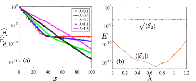
Figure 5: (a) The behaviour of the disorder-average single particle components for different amounts of on-site disorder $\lambda$. The cleaner systems show an exponential decay that follows the non interacting coherence length near the boundary, which revert to a more moderate decay in the bulk. Disorder typically increases the effective single particle coherence length near the boundary while reducing the residual decay lengths in the bulk. (b) For a long enough wire we can see this behaviour is correlated with the disorder averaged $\mathcal{E}_{1}\sim\langle\delta\rangle$ estimate. In contrast this behaviour is clearly not correlated with the $\langle\mathcal{E}_{2}\rangle$ estimate, which is expected to be dominated by non-diagonal disorder $\chi_{2}$. This data is for Region II ($\Delta=0.5t$ and $\mu=-t$) with $U=0.01t$ and bond dimension $\chi=64$

Energy splitting statistics: The previous results outlined how the degree of localization of the approximate zero mode depends on the amount of disorder. Figure 5 shows the correlation between these spatial decay rates and the mean energy splitting estimate $\mathcal{E}_{1}\sim\langle\delta\rangle$ in Region II. The single particle components show clearly the dual nature of disorder. On a mean field level, disorder extends the effective coherence length. This is manifested in a moderation of the exponential decay near the chain edge, which follows the non interacting spatial profile. Conversely, the residual non exponential decay, absent in a non interacting system, is progressively reduced in a disordered medium, see Figure 5 (a). In a long chain, contributions from these non-exponential tails dominate the mean pairwise energy splitting $\mathcal{E}_{1}\sim\langle\delta\rangle$. As such the mean energy-splitting is decreased by moderate disorder, see Figure 5 (b). As disorder is increased further, the single-particle effect dominates and $\mathcal{E}_{1}$ increases.

Figure 5 (b) also shows the associated $\langle\mathcal{E}_{2}\rangle^{1/2}$ estimate. Although this number is expected to be dominated by $\chi_{2}$ in this regime, it does represent an upper bound on the expected spread of the distribution (see discussion about errors in the Appendix B). To address these statistics more directly, in Appendix C we also examine distributions for small systems using exact diagonalisation. We find that disorder reduces the occasional large energy splitting from real decay transitions, but that the standard deviation (about the mean) of pairwise splitting shows only a modest initial decrease with disorder, eventually being overcome due to the increase in the probability of bands to overlap and/or the single particle effect which dominates near the system edges.

Discussion of Multi-particle weights: As a last measure we analyse the total multi-particle content of the zero mode wave function. For this purpose we define the integrated weight in a given $n$-particle sector as the sum of all $n$ particle terms: $|N_{n}|^{2}=\int|u^{(n)}(\vec{x})|^{2}d\vec{x}$, which have the property that $\sum_{n}|N_{n}|^{2}=1$. The total multi-particle content of the zero mode wave function is then given by $1-|N_{1}|^{2}$. It has been argued previously that operators with larger weights in these multi-particle sectors decohere more quickly Goldstein2012 , it could be used as a signature for localization-enhanced topological order, see Ref. Kells2015b, and Appendix D.

Figure 6 shows the distribution of these multi-particle weights as a function of disorder. In Region I we find that disorder increases the multi-particle weight. Region II shows a more intricate behavior. Here, while disorder broadens the distribution thus allowing for specific disorder realisations with a smaller multi-particle weight, both the mean (red-line) and median (black-dashed line) exhibit a monotonic increase.

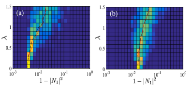
Figure 6: Distributions of the multi-particle content $1-|N_{1}|^{2}$ of the approximate steady state as a function of disorder strength $\lambda$, for (a) Region I ($\Delta=0.7t$ and $\mu=-0.2t$) and (b) Region II ($\Delta=0.5t$ and $\mu=-t$). The plots were obtained for a system of length $L=100$, using an interaction strength $U=0.1t$ and constant MPS bond dimension of $\chi=128$. In Region I the $1-|N_{1}|^{2}$ probability distribution displays a hard minimum and disorder can only increase the weight supported in the multi-particle sectors. In Region II we see that disorder has a chance to increase or decrease the multi-particle weight. Mean and median values are shown in red and black dashed lines respectively)

Conclusion We study numerically the effect of disorder on the stability of the many body zero mode in a Kitaev chain with local interactions. Our methodology allows us to obtain information about the spatial and multi-particle profile of the zero mode operator, as well as to approximate the statistics of nearly degenerate pairs of states associated with the zero mode, over the entire energy spectrum. Our analysis shows that the parameter space of a clean system can be divided into regions where relevant interaction-induced decay transitions are suppressed (Region I) and were they are not (Region II). We find that the effect of disorder on the many body zero mode varies qualitatively between these two regimes. In Region I, disorder has an overall adverse effect: it extends both single particle and multi-particle components further into the bulk while simultaneously increases the likelihood that real decay processes occur. In Region II disorder has a more intricate effect. While broadening exponential decay of the single particle components of the zero mode operator, we observe that local-clusters of multi-particles decay more rapidly in a disordered medium. This more rapid decay is reflected in the mean energy splitting between pairs of states of opposite parity which exhibits an overall reduction in a disordered medium.

The qualitative prediction is that these localization effects should also result in a decrease in the width of the energy splitting distribution - resulting in a many-body Majorana operator that is more mode-like. For larger systems we argue that the MPS measure, which could in-principle be used to address the width of the splitting distribution, are in fact dominated by non-zero mode contributions. However, using exact diagonalisation we show that disorder can reduce the size of the occasional large splitting corresponding to real decay transitions. We note however that this effect is counteracted by an increase in the likelihood of these decay transitions occurring and non-interacting single particle effects which tend to dominate near the system’s edges.

We have discussed in some detail how the enhancement effect ties in with the phenomena of many-body-localization. We note that although the underlying mechanisms and the techniques used to study them are similar, there are important distinctions that result in the phenomena being independent of each other. This can be seen quite clearly in the numerical analysis where we show that measures of MBL cannot resolve the disorder-driven topological phase transition, nor the subtle distinctions between Regions I and II. We stress however that there is nothing in our work that precludes the coexistence of SPT-order and MBL.

The MPS/super-operator methodology can be extended to other related models e.g the proximity coupled models or the $\mathbb{Z}_{n}$ parafermionic clock models. For the class of proximity coupled systems the extension should be possible as these systems also possess a natural non-interacting limit and disorder is known to localise bulk eigenmodes there also. One possible caveat is that in proximity coupled systems, the Kitaev-chain arises as an effective low-energy limit, and it is not clear that the correspondence holds at higher energies.

For the $\mathbb{Z}_{n}$ models, apart from some special cases (e.g. Moran2017 ) there are no obvious non-interacting limits. There are however a number of works that point to exactly-solvable/free-fermion ground-states Iemini2017 ; Meichanetzidis2017 Moreover, there are clear indications that special points of clean $\mathbb{Z}_{n}$ models, where $n$ is prime, can contain strong-zero-modes. One particularly strong candidate for this is the so called $\pi/6$ point in the $\mathbb{Z}_{3}$ system Jermyn2014 ; Moran2017 ; Else2017 . These special points are natural analogs of Region I and so we expect that these models should share many of the same features with the interacting Kitaev chain.

Acknowledgments The authors acknowledge Yevgeny Bar Lev, Piet Brouwer, Dimitri Gutman, Arbel Haim, Falko Pienkta, Domenico Pellegrino, Maria-Theresa Rieder, Alessandro Romito and Joost Slingerland for fruitful discussions. G.K. acknowledges support from Science Foundation Ireland under its Career Development Award Programme 2015, (Grant No. 15/CDA/3240). N.M. acknowledges financial support from Science Foundation Ireland through Principal Investigator Award (Grant No. 12/IA/1697). D. M. acknowledges support from the Israel Science Foundation (Grant No. 737/14) and from the People Programme (Marie Curie Actions) of the European Union’s Seventh Framework Programme (FP7/2007-2013) under REA grant agreement No. 631064. We also wish to acknowledge the SFI/HEA Irish Centre for High-End Computing (ICHEC) for the provision of computational facilities and support.

Appendix A Perturbative zero-modes for finite wires

The argument given in Ref. Kells2015a, shows that the existence of the non-interacting Majorana mode also places restrictions on the form of all couplings between eigenstates of the non-interacting system. The argument relies on the fact the perturbative terms due to local parity-preserving operators will be identical in each sector, provided the states involved have the same zero-mode occupation. As a result, the degenerate perturbation expansions of the bands themselves will look the same in each sector, to an order of perturbation theory that scales with the length of the system ( see also Ref. Moran2017, ). However, this argument does not account for situations where the bands with different fermion number start to hybridize. In this case interaction-induced transitions between bands with different occupation of the non-interacting zero mode will factor into left $\pm$ right (for even and odd sectors) Kells2015a and therefore when these bands start to intersect we see some even-odd sectoral dependency at avoided level crossings.

This basic argument allows us to place some more simple limits on the degree to which degeneracy is protected in the wire. The single particle spectrum of the non-interacting system is given as $\epsilon_{k}=((-\mu-2t\cos k)^{2}+(2|\Delta|\sin k)^{2})^{1/2}$. For $\mu<0$, such that we move the chemical potential towards the bottom of the band, the maximum bulk-excitation energy is $\epsilon_{\text{max}}=2t-\mu$, and the minimum is

$$\epsilon_{\text{min}}=\begin{cases}2t+\mu,&\text{if }\frac{t}{2}(u+2t)<|\Delta|^{2}\\ |\Delta|\sqrt{4-\frac{\mu^{2}}{(t^{2}-\Delta^{2})}},&\text{otherwise}\end{cases}$$ (15)

The condition that there are no overlaps between bands that differ by one bulk fermion-excitation is that $\epsilon_{\text{max}}<2\epsilon_{\text{min}}$ and we arrive at the inequality which, in the main text, defines our Region I:

$$-\mu<\frac{2}{3}t,\quad\quad\quad\quad\quad\quad\text{if }\frac{t}{2}(u+2t)<|\Delta|^{2}$$

$$-\mu<2(|\Delta|\sqrt{4-\frac{\mu^{2}}{t^{2}-|\Delta|^{2}}}-t),\text{otherwise}$$

We can also estimate when this spread becomes large enough to close the gap $(2t)$ between the $N^{th}$ and $N-1^{th}$ bands. Near the flat band limit ($t=|\Delta|$, $\mu=0$), and with $\mu<0$, the maximum of the band occurs at $\epsilon_{\text{max}}=2t-\mu$ at $k=\pm\pi$ and the minimum occurs roughly at $2|\Delta|\sin k_{F}$ where $k_{F}=\cos^{-1}\mu/2t\approx\pi/2$ and therefore $\epsilon_{\text{min}}\approx 2|\Delta|$. The spread in the single particle spectrum is therefore $|\mu|+\kappa$, with $\kappa\equiv 2(t-|\Delta|)$. Assuming we are in a large enough system such that the $N^{th}$ largest and smallest single particle eigenvalues are almost the same we can write the requirement that the bands don’t overlap : $N\epsilon_{\text{min}}-(N-1)\epsilon_{\text{max}}>0$, which after rearranging becomes

$$\frac{\kappa+|\mu|}{4t+|\mu|}<\frac{1}{N}.$$ (17)

The condition is restrictive. Close to the middle of the spectrum this occurs at at progressively small $\kappa$ and $\mu$. A caveat to this however is that the splitting that occurs between the bands $N$ and $N-1$ (recall that one of these states has an occupied zero mode which we are not counting) comes about because of non-zero matrix elements between states that differ by $\sim 2N$ fermions. As such, the interaction-induced transition that couples these states would therefore result in an even-odd splitting of the order $U^{N/2}$ occurring at this interaction induced avoided level crossing.

Moreover, for a system of length $L$ as we vary $\mu$ or $\kappa$ away from the special point, the first crossing occurs between the $N=L/2$ and say $=N-1=L/2-1$ bands. However as the avoided level crossing here must be proportional to $U^{L/4}$ the even-odd splitting will strictly speaking still be exponential in a parameter that is a sizeable fraction of the system length. The question of whether there is a strong zero mode when both $\mu$ and $\kappa$ are non-zero is therefore a complicated one, and the answer has to be qualified based on where exactly one is in the parameter space.

For a finite wire, we see that there is a finite region of parameter space for non-zero $\mu$ and $\kappa$ such that there is a strong zero mode. Nonetheless, this region diminishes as one approaches the thermodynamic limit. On this point, we note that it is always possible to make the zero mode exact with some small local tweak in parameters near one of the wire ends and thus for many purposes in what follows it is useful to proceed as if there is an exact zero mode and to explore the consequences that this must have for it’s multi-particle content.

Appendix B DMRG for superoperators

Our algorithm attempts to construct multinomials of position space Majorana operators:

$$\gamma_{L}(U)=\sum_{i}^{2L}u^{(1)}_{L}(i)\gamma_{i}+\sum_{ijk}^{2L}u^{(3)}_{L}(i,j,k)\gamma_{i}\gamma_{j}\gamma_{k}+...$$ (18)

$$\gamma^{R}(U)=\sum_{i}^{2L}u^{(1)}_{R}(i)\gamma_{i}+\sum_{ijk}^{2L}u^{(3)}_{R}(i,j,k)\gamma_{i}\gamma_{j}\gamma_{k}+...$$

that almost commute with the interacting Kitaev wire Hamiltonian. These modes are normalised such that if we define weights $N^{n}=\int|u^{(n)}(\vec{x}|^{2}dx$ then $\sum N^{n}=1$ . In the non-interacting system, the expansion coefficients $u^{(n)}=0$ for all $n>1$, and therefore $N^{(1)}=1$. In keeping with the idea of the mode as a dressed quasi-particle, we expect that the single particle weight $N^{(1)}$ dominates the other multi-particle weights also in the case of non-zero interaction strength $U$.

In Ref. Kells2015b, it was demonstrated how one can approximate such a mode using a real space approach that selectively sampled the multi-particle components that were close, in configuration space, to single particle operators. The technique works by creating a matrix representation for the super-operator $\mathcal{H}=[H,\bullet]$ and finding approximate steady states of the form (7) by variationally approaching a single-particle dominated null vector of $\mathcal{H}^{2}$.

One difficulty with this method is that the Hilbert space dimension of null-vectors of $\mathcal{H}$ grows as $2^{L}$ and moreover is itself embedded in a continuum. However, it is possible to argue that within this continuous band of excitation energies there are only two approximate steady-states with the form (7) that are dominated by the single-particle elements. Moreover, by continuity it is straightforward to argue that the single particle components of the operators should have a similar structure to their non-interacting counterparts.

The variational step searches for null vectors of $\mathcal{H}^{2}$ using a Lanczos algorithm. The initial states for the procedure are the non-interacting Majorana’s on both ends of the wires. Working with $\mathcal{H}^{2}$ is needed to ensure our eigenvalue approximation is bounded from below, and has the additional advantage that this operator preserves sub-lattice symmetry. Thin restarting is needed to ensure that on each iteration of the algorithm the updated state resembles the input state.

The algorithm that we use in this paper can be seen as a hybrid of the aforementioned real-space sampling approach and methods that seek to use DMRG approaches to approximate the null-vectors of $\mathcal{H}$ or more generally the Limbladlian Mascarenhas2015 ; Cui2015 . The key difference with the real-space sampling approach is that the operator $\mathcal{H}=[H,\bullet]$ is now represented as a Matrix-Product-Operator. From this we contract indices of the MPO to obtain an MPO for $\mathcal{H}^{2}$ and then search for its null-vectors using a modified DMRG sweeping procedure.

To ensure that algorithm converges to the single-particle dominated modes we found it necessary to again employ Lancsoz thin-restarting, this time at each optimisation step in the sweep along the wire/chain. In terms of overall efficiency we note that orders of magnitude improvement can be obtained by also implementing a controlled compression of the MPO $\mathcal{H}^{2}$.

B.1 Discussion of numerical errors in the MPS variational technique

In the main text we argued that the MPO/MPS representation of the zero-mode could be written in the eigenbasis of the Hamiltonian as:

$$\Gamma_{L} =\sum_{n}(1-\alpha^{L}_{n})\left[|n_{0}\rangle\langle n_{1}|+|n_{1}\rangle\langle n_{0}|\right]$$ (19)

$$+\sum_{n\neq m}\beta^{L}_{nm}\left[|n_{0}\rangle\langle m_{1}|+|m_{1}\rangle\langle n_{0}|\right]$$

$$\Gamma_{R} =-i\sum_{n}(1-\alpha^{R}_{n})\left[|n_{0}\rangle\langle n_{1}|-|n_{1}\rangle\langle n_{0}|\right]$$ (20)

$$-i\sum_{n\neq m}\beta^{R}_{nm}\left[|n_{0}\rangle\langle m_{1}|-|m_{1}\rangle\langle n_{0}|\right]$$

where the $\alpha$ and $\beta$-terms represent diagonal/off-diagonal errors respectively. Moreover we showed that the estimates for the energy level statistics are calculated using the trace formula:

$$\mathcal{E}_{1}=i\operatorname{Tr}(\Gamma_{L}\times[H,\Gamma_{R}])/2^{L}=\langle\delta\rangle+\chi_{1}$$ (21)

$$\mathcal{E}_{2}=\operatorname{Tr}(\Gamma_{L}\times[H,[H,\Gamma_{L}]])/2^{L}=\langle\delta^{2}\rangle+\chi_{2}$$ (22)

where

$$\chi_{1} =-\frac{1}{2^{L}}\sum_{n}\delta_{n}\left[\alpha^{L}_{n}+\alpha^{R}_{n}-\alpha^{L}_{n}\alpha^{R}_{n}\right]$$ (23)

$$+\frac{1}{2^{L}}\sum_{n\neq m}\beta^{L}_{nm}\beta^{R}_{nm}[E_{n}-E_{m}+\frac{\delta_{n}}{2}+\frac{\delta_{m}}{2}]$$

and

$$\chi_{2} =-\frac{1}{2^{L}}\sum_{n}\delta_{n}^{2}(2\alpha^{L}_{n}-(\alpha^{L}_{n})^{2})$$ (24)

$$+\frac{1}{2^{L}}\sum_{n\neq m}(\beta^{L}_{nm})^{2}[E_{n}-E_{m}+\frac{\delta_{n}}{2}+\frac{\delta_{m}}{2}]^{2}.$$

Here, the error $\chi_{1}$ is an average over small contributions of random sign. We therefore expect it to be negligible. In contrast $\chi_{2}$ can dominate the second moment $\mathcal{E}^{2}$.

To check this conjecture, we perform the following simple test. At fixed bond dimension we compare the asymptotic value of the $\mathcal{E}_{2}$(calculated using the $\Gamma_{L}$ operator) with the asymptotic value of a almost identical set up, given by Eq. (1) and (2) where the coupling terms on the very right hand side of the system are changed to ensure we have a perfectly decoupled $\Gamma_{R}=\gamma_{2N}$ Majorana (e.g we set $\mu_{N}=0$, $\Delta_{N-1}=t\arg(\Delta)$ and $U_{N-1}=0$ ). In the modified setup, as a result of the perfectly decoupled $\Gamma_{R}$ Majorana, the true many body spectrum is exactly two fold degenerate, which corresponds to Eq. (II), with $\delta_{n}=0$ for all $n$. In this setup, the first and second moments are determined solely by the off diagonal errors in $\chi_{1}$ and $\chi_{2}$:

$$\mathcal{E}_{1}=\chi_{1} =\frac{1}{2^{L}}\sum_{n\neq m}\beta^{L}_{nm}\beta^{R}_{nm}[E_{n}-E_{m}]$$ (25)

and

$$\mathcal{E}_{2}=\chi_{2} =\frac{1}{2^{L}}\sum_{n\neq m}(\beta^{L}_{nm})^{2}[E_{n}-E_{m}]^{2}.$$ (26)

Moreover, in the modified setup, the right Majorana can be determined exactly, and $\alpha^{R}=\beta^{R}=0$. Consequently, the resulting first moment $\mathcal{E}$ will be identically zero, regardless of the numerically calculated $\Gamma_{L}$.

In contrast the estimate for $\mathcal{E}_{2}$ are affected by errors of the calculated $\Gamma_{L}$ only and do not necessarily vanish. We find that the estimate for the second moment $\mathcal{E}_{2}$ in the modified setup with an exact degeneracy and in the original setup given by Eq. (1) and (2) to be comparable. This supports our conjecture that the second moment calculations are dominated by off diagonal errors.

Figure 7 shows the distribution of $\mathcal{E}_{2}$ as a function of disorder in (a) Region I and (b) Region II. A similar calculation in the modified setup gives comparable results which indicates that the value of $\mathcal{E}_{2}$ is dominated by off diagonal error $\chi_{2}$. Moreover, the data taken in the modified setup show a similar trend with disorder. This suggest that $\mathcal{E}_{2}$ and consequently $\chi_{2}$ generally reflect the extent of mixing between bands. In this respect we see for example that in Region I disorder substantially increases the $\mathcal{E}_{2}$ estimate, indicating that it drives the system into the regime where real transitions can occur. In Region II the $\mathcal{E}_{2}$ estimate shows a moderate increase with disorder, in accordance with the expectation that it is determined by the degree of mixing between bands.

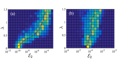
Figure 7: Distributions of $\mathcal{E}_{2}$ as a function of disorder strength $\lambda$, for (a) Region I ($\Delta=0.7t$ and $\mu=-0.2t$) and (b) Region II ($\Delta=0.5t$ and $\mu=-t$). The plots were obtained for a system of length $L=100$, using an interaction strength $U=0.1t$ and constant MPS bond dimension of $\chi=64$. One hundred disorder realisations are used for each value of $\lambda$. In Region I the dominant effect of disorder is to push the system towards values closer to those observed in Region II. In Region II we see that disorder has a chance to increase or decrease the $\mathcal{E}_{2}$. We observe that the average and median values (red and black dashed lines resp.) tend to increase as we increase the amount of disorder.

Appendix C Measures of localization enhanced topological order in Exact-Diagonalisation calculations

Interaction induced decay transitions, which can change the occupancy of the zero mode while exciting Bogoliubov quasi-particles, occur when bands of different fermion occupation number cross. The key prediction of localization enhanced topological order, is that the resulting mismatch in even-odd energy levels at the avoided crossings (see Figure 9) will become smaller as the amount of disorder is increased.

In exact diagonalisation this effect is quite difficult to discern in the overall energy level splitting statistics. This is because, in the parameter space accessible to exact diagonalisation (ED) (large $\Delta$), disorder increases (on average) both the overall splitting of pairs as well as the probability that an anomalous splitting can occur. The effect on the average splitting can be understood on a single particle level as resulting from the increases in the effective coherence length in a disordered medium. The increase in the number of anomalous splittings comes about because disorder will also broaden the bands and hence increase the chances that bands with different fermion number overlap. Hence, while disorder reduces the value of anomalous pair splitting, it increases their number.

For small system size, the latter explains qualitatively why one should not necessarily observe a reduction in the global statistical quantities such as $\text{Var}(\delta)$ even though the responsible matrix elements should be reduced by disorder (see Figure 8) for the corresponding calculation for $L=13$). The ED calculations, however, allow us to calculate the entire probability distribution of energy levels. Here the reduction in decay like transitions, becomes apparent in the shape of the distributions at higher-pair splitting.

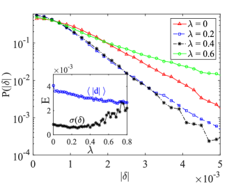
Figure 8: For small system sizes the disorder averaged distribution $P(\delta)$ can become less broad with a modest amount of disorder. This is because, even for very small systems sizes ($L=13$) the matrix elements responsible for real decay processes are reduced as a function of disorder parameter $\lambda$. The effect quickly disappears as one increases disorder because this (on-average) drives the system further into Region II and also increase the single-particle coherence length of the Majorana end-states (an effect which is more relevant for short systems). The inset shows the standard deviation $\sigma(\delta)$, calculated using the full spectrum, and the $\langle|d|\rangle$ is the mean of all interacting matrix elements (in the non-interacting basis) that differ by occupation of the zero-mode . The data was generated in Region II, with $\mu=-1,\Delta=0.5t$ and $U=0.1t$.

Appendix D Formal Majorana construction and the connection between the energy splitting and multi-particle content

In terms of the eigenstates of the system we can write

$$\gamma_{L}(U) =\phantom{i}\sum|\,n_{0}\rangle\langle n_{1}\,|+|\,n_{1}\rangle\langle n_{0}\,|$$ (27)

$$\gamma_{R}(U) =i\sum|\,n_{0}\rangle\langle n_{1}\,|-|\,n_{1}\rangle\langle n_{0}\,|.$$ (28)

where the sub-script the approximate occupation of the zero-mode. This method of constructing the modes is formally identical to the method of l-bit construction in the MBL literature, see for example Ref. Huse2014, , and requires one to be able to identify pairs of states $|\,n_{0}\rangle$ and $|\,n_{1}\rangle$ , and then to fix the relative phases. One way to make this identification in principle is to use the energy of the states as an identifier and match states according to where they occur in the energy spectrum. Another identification method is to examine how well two states are mapped to each other by the non-interacting modes,which can be calculated exactly:

$$O_{L/R}=\langle n_{\text{even}}\,|\gamma_{L/R}(0)|\,m_{\text{odd}}\rangle$$ (29)

This latter method also allows one to determine the correct relative phase.

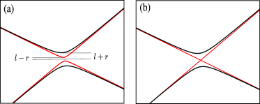
Figure 9: At crossings between states with different (approximate) occupations of the zero-mode, the interaction dependent splitting coefficient factors in to a left and right contribution (see e.g. Kells2015a ). In the presence of disorder, the average splitting coefficients $l$ and $r$ should decay exponentially with the system length $L$. (b) In a clean system with perfect reflection symmetry about the centre of the wire one of the sectors, depending on the total fermionic and spatial parity, will always display a symmetry protected crossing.

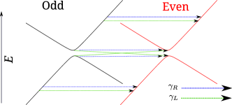
Figure 10: In order to construct the many-body Majorana zero mode one needs to first identify which states in each sector to pair up. Away from the avoided crossings this identification can be achieved either by examining the energy or by using the non-interacting Majorana modes $\gamma_{L/R}(0)$. At the crossing however, one of the non-interacting modes (in this figure we have chosen $\gamma_{L}(0)$) will always identify states at the other side of the crossing. This sets up the relationship between multi-particle content and energy.

In the case of well separated fermionic bands both identification criteria ($E$ and $O_{L/R}$) are in agreement. However, band crossings may introduce an ambiguity between these methods of identification . This has implications for the zero-mode’s residual energy and its multi-particle content.

To see this, consider what happens at an avoided crossings between states from the same parity sector that differ in their occupation of the zero mode. Working in the basis $|\,n\rangle_{0/1}$, $|\,n+1\rangle_{1/0}$, we can understand the crossing point using the following parametrization of the matrix elements between the relevant states

$$H_{c}=E_{c}+\left[\begin{array}[]{cc}as&l\pm r\\ l\pm r&bs\end{array}\right]$$ (30)

where $s$ is related to the parameters of the non-interacting Hamiltonian ($\mu$, $\Delta$, $t$), and $a$ and $b$ are the slopes of the energy levels at the crossing. Here the off-diagonal elements $d_{e,o}=l\pm r$ are the interaction-induced coupling coefficients in the even and odd parity sectors, respectively, which are generally different. The partition into left (l) and right (r) components comes about because the states in question differ in the occupation of the fermionic zero mode $\beta_{0}^{\dagger}\beta_{0}$ and thus we need to operate with either $\beta_{0}=\gamma_{L}+i\gamma_{R}$ or $\beta^{\dagger}_{0}=\gamma_{L}-i\gamma_{R}$ to connect them.

The question we now ask is which states are identified as pairs by the non-interacting Majoranas $\gamma_{L}(0)$ and $\gamma_{R}(0)$? Away from the crossings the relevant eigen-subspace is $|\,\psi_{e}\rangle=\{|\,n\rangle_{0},|\,n+1\rangle_{1}\}$ and $|\,\psi_{o}\rangle=\{|\,n\rangle_{1},|\,n+1\rangle_{0}\}$ where $e/o$ denotes the even/odd sector and $0/1$ denote the approximate occupation of the zero mode. In this basis we have

$$\langle\psi_{e}\,|\gamma_{L}(0)|\,\psi_{o}\rangle\sim I\quad\langle\psi_{e}\,|\gamma_{R}(0)|\,\psi_{o}\rangle\sim\sigma^{z}.$$

At the crossing, the interaction lifts the degeneracy and the modified eigenbasis is rotated to symmetric and antisymmetric combinations: $|\,\tilde{\psi}_{e}\rangle=\{|\,n\rangle_{0}\pm|\,n+1\rangle_{1}\}$ and $|\,\tilde{\psi}_{o}\rangle=\{|\,n\rangle_{1}\pm|\,n+1\rangle_{0}\}$. Therefore in this scenario one of the non-interacting Majoranas will always identify with a state at the other side of the crossing: For the particular example when $l\pm r>0$ we get

$$\langle\tilde{\psi}_{e}\,|\gamma_{L}(0)|\,\tilde{\psi}_{o}\rangle\sim I\quad\langle\tilde{\psi}_{e}\,|\gamma_{R}(0)|\,\tilde{\psi}_{o}\rangle\sim\sigma_{x},$$

implying that the non-interacting left Majorana connects states in opposite parity sectors, with an energy splitting of the same sign $\pm\Delta_{e}\xrightarrow{\gamma_{L}}\pm\Delta_{o}$ while the non-interacting right Majorana identifies states with energy splitting of an opposite sign $\pm\Delta_{e}\xrightarrow{\gamma_{R}}\mp\Delta_{o}$. (In cases when $l\pm r<0$ results in a similar scenarios where it is $\gamma_{L}(0)$ that identifies states on opposite side of the crossing).

More insight can be gained by considering the scenario where one artificially forces one side of the system (say the right) to be non-interacting. This ensures that the single-particle $\gamma_{R}(0)$ Majorana is an exact zero-mode. Moreover, in this scenario all the interaction-induced coupling coefficient $r$ at the r.h.s vanish identically, and the splitting in both sectors is identical. By construction, $\gamma_{R}(0)$ will identify states at the same energy, even in the case where there is an avoided crossing. However, at the crossing point, the non-interacting Majorana at the left hand side will identify states with an energy mismatch, see again Figure 10.

This highlights the ambiguity between constructing a near-zero mode operator which pairs up states of opposite parity with a minimal energy mismatch, or near zero mode which operates similarly to its non interacting counter part. As an example, in the modified setup described above, we may construct an operator $\gamma_{L}(U)$ using states $|\,n\rangle_{e}$ and $|\,n\rangle_{o}$ which are identified by the non interacting $\gamma_{L}(0)$. The resulting operator would connect states with an energy mismatch - in other words it is not a zero mode. On the other hand, constructing an operator out of states with identical energies would result in a zero-mode by definition, but the states chosen to appear together in the outer product are very different from the ones that are suggested by the single-particle $\gamma_{L}(0)$. As such, we can construct a zero-mode but with the price that the operator does not resemble the non-interacting mode within this subspace.

References

- (1) N. Read and D. Green, Paired states of fermions in two dimensions with breaking of parity and time-reversal symmetries and the fractional quantum Hall effect, Phys. Rev. B 61, 10267 (2000).
- (2) D. A. Ivanov, Non-Abelian Statistics of Half-Quantum Vortices in p-Wave Superconductors Phys. Rev. Lett. 86, 268 (2001).
- (3) A. Y. Kitaev, Unpaired Majorana fermions in quantum wires, Phys. Usp. 44, 131 (2001).
- (4) A. Y. Kitaev, Anyons in an exactly solved model and beyond, Ann. Phys. 321 2 (2006).
- (5) C. Nayak, S. H. Simon, A. Stern, M. Freedman, and S. Das Sarma, Non-Abelian anyons and topological quantum computation, Rev. Mod. Phys. 80, 1083 (2008).
- (6) L. Fu, C. L. Kane, Superconducting Proximity Effect and Majorana Fermions at the Surface of a Topological Insulator, Phys. Rev. Lett. 100 096407 (2008).
- (7) R. M. Lutchyn, J. D. Sau, S. Das Sarma, Majorana Fermions and a Topological Phase Transition in Semiconductor-Superconductor Heterostructures, Phys. Rev. Lett. 105 077001 (2010).
- (8) Y. Oreg, G. Refael, F. von Oppen, Helical Liquids and Majorana Bound States in Quantum Wires, Phys. Rev. Lett. 105 177002 (2010).
- (9) M. Duckheim and P.W. Brouwer, Andreev reflection from noncentrosymmetric superconductors and Majorana bound-state generation in half-metallic ferromagnets, Phys. Rev. B 83, 054513 (2011).
- (10) S. B. Chung, H.-J. Zhang, X.-L. Qi, and S.-C. Zhang, Topological superconducting phase and Majorana fermions in half-metal/superconductor heterostructures, Phys. Rev. B 84, 060510 (2011).
- (11) T.-P. Choy, J. M. Edge, A. R. Akhmerov, and C. W. J. Beenakker, Majorana fermions emerging from magnetic nanoparticles on a superconductor without spin-orbit coupling, Phys. Rev. B 84, 195442 (2011).
- (12) M. Kjaergaard, K. Wölms, and K. Flensberg, Majorana fermions in superconducting nanowires without spin-orbit coupling, Phys. Rev. B 85, 020503 (2012).
- (13) I. Martin and A. F. Morpurgo, Majorana fermions in superconducting helical magnets, Phys. Rev. B 85, 144505 (2012).
- (14) S. Nadj-Perge, I. K. Drozdov, B. A. Bernevig, and A. Yazdani, Proposal for realizing Majorana fermions in chains of magnetic atoms on a superconductor, Phys. Rev. B 88, 020407(R) (2013).
- (15) V. Mourik, K. Zuo, S. M. Frolov, S. R. Plissard, E. P. A. M. Bakkers, and L. P. Kouwenhoven, Signatures of Majorana Fermions in Hybrid Supercondcutor-Semiconductor Nanowire Devices, Science 336, 1003 (2012).
- (16) M. T. Deng, C. L. Yu, G. Y. Huang, M. Larsson, P. Caroff, and H. Q. Xu, Anomalous zero-bias conductance peak in a Nb-InSb nanowire-Nb hybrid device, Nano Lett. 12, 6414 (2012).
- (17) A. Das, Y. Ronen, Y. Most, Y. Oreg, M. Heiblum, and H. Shtrikman, Zero-bias peaks and splitting in an Al-InAs nanowire topological superconductor as a signature of Majorana fermions Nat. Phys. 8, 887 (2012).
- (18) A. D. K. Finck, D. J. Van Harlingen, P. K. Mohseni, K. Jung, and X. Li, Anomalous modulation of a zero-bias peak in a hybrid nanowire- superconductor device, Phys. Rev. Lett. 110, 126406 (2013).
- (19) H. O. H. Churchill, V. Fatemi, K. Grove-Rasmussen, M. T. Deng, P. Caroff, H. Q. Xu, and C. M. Marcus, Superconductor-nanowire devices from tunneling to the multichannel regime: Zero-bias oscillations and magnetoconductance crossover, Phys. Rev. B 87, 241401 (2013).
- (20) S. M. Albrecht, A. P. Higginbotham, M. Madsen, F. Kuemmeth, T. S. Jespersen, J. N. rd, , P. Krogstrup, and C. M. Marcus, Exponential protection of zero modes in Majorana islands, Nature 531, 206 (2016).
- (21) H. Zhang, Ö. Gül, S. Conesa-Boj, K. Zuo, V. Mourik, F. K. de Vries, J. van Veen, D. J. van Woerkom, M. P. Nowak, M. Wimmer, D. Car, S. Plissard, E. P. A. M. Bakkers, M. Quintero-Pérez, S. Goswami, K. Watanabe, T. Taniguchi, L. P. Kouwenhoven, Ballistic Majorana nanowire devices, arXiv:1603.04069 (2016).
- (22) M. T. Deng, S. Vaitiekėnas, E. B. Hansen, J. Danon, M. Leijnse, K. Flensberg, J. Nygård, P. Krogstrup, and C. M. Marcus, Majorana bound state in a coupled quantum-dot hybrid-nanowire system, Science 354, 1557 (2016).
- (23) S. Nadj-Perge, I. K. Drozdov, J. Li, H. Chen, S. Jeon, J. Seo, A. H. MacDonald, B. A. Bernevig, and A. Yazdani Observation of Majorana fermions in ferromagnetic atomic chains on a superconductor, Science 346 602 (2014).
- (24) M. Ruby, F. Pientka, Y. Peng, F. vonOppen, B. W. Heinrich, and K. J. Franke, End States and Subgap Structure in Proximity-Coupled Chains of Magnetic Adatoms, Phys. Rev. Lett. 115, 197204 (2015).
- (25) R. Pawlak, M. Kisiel, J. Klinovaja, T. Meier, S. Kawai, T. Glatzel, D. Loss, and E. Meyer, Probing atomic structure and Majorana wavefunctions in mono-atomic Fe chains on superconducting Pb surface, Npj Quantum Inf. 2, 16035 (2016).
- (26) O. Motrunich, K. Damle, and D. A. Huse, Griffiths effects and quantum critical points in dirty superconductors without spin-rotation invariance: One-dimensional examples, Phys. Rev. B 63, 224204 (2001).
- (27) P. W. Brouwer, M. Duckheim, A. Romito and F. von Oppen, Probability distribution of Majorana end-state energies in disordered wires, Phys. Rev. Lett. 107, 196804 (2011).
- (28) P. W. Brouwer, M. Duckheim, A. Romito and F. von Oppen, Topological superconducting phases in disordered quantum wires with strong spin-orbit coupling, Phys. Rev. B 84, 144526 (2011).
- (29) A. R. Akhmerov, J. P. Dahlhaus, F. Hassler, M. Wimmer, and C. W. J. Beenakker, Quantized Conductance at the Majorana Phase Transition in a Disordered Superconducting Wire, Phys. Rev. Lett. 106, 057001 (2011).
- (30) M.-T. Rieder, G. Kells, M. Duckheim, D. Meidan, and P. W. Brouwer, Endstates in multichannel spinless p-wave superconducting wires, Phys. Rev. B 86, 125423 (2012).
- (31) M.-T. Rieder, P. W. Brouwer and I. Adagideli, Reentrant topological phase transitions in a disordered spinless superconducting wire, Phys. Rev. B 88, 060509(R) (2013).
- (32) W. DeGottardi, D. Sen and S. Vishveshwara, Majorana fermions in superconducting 1D systems having periodic, quasiperiodic, and disordered potentials Phys. Rev. Lett. 110, 146404 (2013).
- (33) F Pientka, A. Romito, M. Duckheim, Y. Oreg and F. von Oppen, Signatures of topological phase transitions in mesoscopic superconducting rings, New Journal of Physics 15 025001 (2013).
- (34) E. M. Stoudenmire, J. Alicea, O. A. Starykh, and M. P. A. Fisher, Interaction effects in topological superconducting wires supporting Majorana fermions, Phys. Rev. B 84, 014503 (2011).
- (35) E. Sela, A. Altland, and A. Rosch, Majorana fermions in strongly interacting helical liquids Phys. Rev. B 84, 085114 (2011).
- (36) R. M. Lutchyn and M. P. A. Fisher, Interacting topological phases in multiband nanowires Phys. Rev. B 84, 214528 (2011).
- (37) A. M. Lobos, R. M. Lutchyn, S. Das Sarma, Interplay of disorder and interaction in majorana quantum wires, Phys. Rev. Lett. 109, 146403 (2012).
- (38) F. Crépin, G. Zaránd and P. Simon, Nonperturbative phase diagram of interacting disordered Majorana nanowires, Phys. Rev. B 90, 121407(R) (2014).
- (39) F. Hassler and D. Schuricht, Strongly interacting Majorana modes in an array of Josephson junctions New J. Phys. 14, 125018 (2012).
- (40) R. Thomale, S. Rachel, and P. Schmitteckert, Tunneling spectra simulation of interacting Majorana wires, Phys. Rev. B 88, 161103(R) (2013).
- (41) H. Katsura, D. Schuricht, M. Takahashi, Exact ground states and topological order in interacting Kitaev/Majorana chains, Phys. Rev. B 92, 115137 (2015).
- (42) N. M. Gergs, L. Fritz, and D. Schuricht Topological order in the Kitaev/Majorana chain in the presence of disorder and interactions Phys. Rev. B 93, 075129 (2016).
- (43) S. Gangadharaiah, B. Braunecker, P. Simon and D. Loss, Majorana edge states in interacting one-dimensional systems, Phys. Rev. Lett. 107, 036801 (2011).
- (44) G. Goldstein and C. Chamon, Exact zero modes in closed systems of interacting fermions, Phys. Rev. B. 86, 115122 (2012).
- (45) P. Fendley, Strong zero modes and eigenstate phase transitions in the XYZ/interacting Majorana chain J. Phys. A: Math. Theor. 49 30LT01 (2016).
- (46) M. McGinley, J. Knolle, and A. Nunnenkamp, Robustness of Majorana edge modes and topological order - exact results for the symmetric interacting Kitaev chain with disorder, arXiv:1706.10249
- (47) J.-J. Miao, H.-K. Jin, F.-C. Zhang, and Y. Zhou, Exact Solution for the Interacting Kitaev Chain at the Symmetric Point Phys. Rev. Lett. 118, 267701 (2017).
- (48) G. Kells, Many-body Majorana operators and the equivalence of parity sectors, Phys. Rev. B 92, 081401(R) (2015).
- (49) J. Kemp, N. Y. Yao, C. R. Laumann and P. Fendley, Long coherence times for edge spins, J. Stat. Mech. 063105 (2017).
- (50) N. Moran, D. Pellegrino, J. K. Slingerland and G. Kells, Parafermionic clock models and quantum resonance, Phys. Rev. B 95, 235127 (2017).
- (51) D. V. Else, P. Fendley, J. Kemp and C. Nayak, Prethermal Strong Zero Modes and Topological Qubits, Phys. Rev. X 7, 041062 (2017)
- (52) P. Fendley, Parafermionic edge zero modes in -invariant spin chains, J. Stat. Mech. 2012, 11020 (2012).
- (53) P. Fendley Free parafermions, J. Phys. A: Math. Theor. 47 075001 (2014).
- (54) A. S. Jermyn, R. S. K. Mong, J. Alicea, and P. Fendley, Phys. Rev. B 90, 165106 (2014).
- (55) G. Kells, Multiparticle content of Majorana zero modes in the interacting p -wave wire, Phys. Rev. B 92, 155434 (2015).
- (56) The case for strong zero-modes can be made in several exactly solvable limits see e.g Ref. Gangadharaiah2011, ; Goldstein2012, ; Fendley2016, ; McGinely2017, and can be extended into other regimes as long as there is no energetic overlap between bands with different fermion numberKells2015a ; Kemp2017 ; Moran2017 ; Else2017 .
- (57) For studies of the same phenomena in the context of parafermionic clock models see Ref. Fendley2012, ; Fendley2014, ; Jermyn2014, ; Moran2017, .
- (58) I.V. Gornyi, A.D. Mirlin and D. G. Polyakov, Interacting electrons in disordered wires: Anderson localization and low-T transport, Phys. Rev. Lett. 95, 206603 (2005).
- (59) D.M. Basko, I. L. Aleiner and B. L. Altshuler, Metal-insulator transition in a weakly interacting many-electron system with localized single-particle states, Annals of Physics 321, 1126 (2006).
- (60) D. A. Huse, R. Nandkishore, V. Oganesyan, A. Pal, and S. L. Sondhi, Localization-protected quantum order Phys. Rev. B 88, 014206 (2013).
- (61) B. Bauer and C. Nayak, Area laws in a many-body localized state and its implications for topological order J. Stat. Mech. P09005 (2013).
- (62) A. Chandran, V. Khemani, C. R. Laumann, and S. L. Sondhi, Many-body localization and symmetry-protected topological order, Phys. Rev. B 89, 144201 (2014).
- (63) J. A. Kjäll, J. H. Bardarson, and F. Pollmann, Many-body localization in a disordered quantum ising chain, Phys. Rev. Lett. 113, 107204 (2014).
- (64) A. Carmele, M. Heyl, C. Kraus and M. Dalmonte, Stretched exponential decay of Majorana edge modes in many-body localized Kitaev chains under dissipation, Phys. Rev. B 92, 195107 (2015).
- (65) Y. Bahri, R. Vosk, E. Altman, and A. Vishwanath, localization and topology protected quantum coherence at the edge of hot matter Nat. Commun. 6, 7341 (2015).
- (66) J. R. Wootton and J. K. Pachos, Bringing order through disorder: localization of errors in topological quantum memories, Phys. Rev. Lett. 107, 030503 (2011).
- (67) S. Bravyi and R. Koenig, Disorder-Assisted Error Correction in Majorana Chains, Comm. Math. Phys., 316 (3), 641 (2012).
- (68) C. Stark, L. Pollet, A. Imamoğlu and Renato Renner, localization of toric code defects, Phys. Rev. Lett, 107, 030504 (2011).
- (69) A. C. Potter and R. Vasseur Symmetry constraints on many-body localization, Phys. Rev. B 94, 224206 (2016).
- (70) Within the literature, the enhancement of topological-order can have a number of distinct meanings. With respect to the ground state properties it is well known that disorder Pientka2013 , interactions Stoudenmire2011 and combinations of both Gergs2016 can shift the boundary of the topological region. In instances where the system is already close to the topological phase transition this can have a stabilising effect. However, the idea of localization-enhanced topological-order as discussed in e.g. Huse2013 ; Bauer2013 ; Kjall2014 ; Carmele2015 ; Bahri2015 ; Wootton2011 ; Stark2011 ; Bravyi2012 ; Chandran2014 ; Potter2016 refers to the behaviour of many-body states at finite energy density. In the context of topological superconductors it is understood as an enhancement of the physical attributes of the pre-existing Majorana modes, on which the topological qubit is based (see e.g. Huse2013 ; Kjall2014 ) . Similarly one can ( e.g. Refs. Bravyi2012 ; Carmele2015 ) focus on the dynamical properties of edge correlators, which can be seen as a indication of how long our qubit remains intact given imperfect knowledge of both the initial quantum state and subsequent dynamical evolution. In these later dynamical cases the notion of localization-enhanced topological-qubit can also include the effects of post-processing/error-correction of the quantum system. We note that for 2D topological memories the presence of disorder is often a necessary ingredient, see for example Wootton2011 ; Stark2011 ; Chandran2014 .
- (71) G. M. Crosswhite and D. Bacon, Finite automata for caching in matrix product algorithms, Phys. Rev. A, 78, 012356 (2008).
- (72) U. Schollwöck, The density-matrix renormalization group in the age of matrix product states, Annals of Physics 326 96 (2011).
- (73) D. A. Huse, R. Nandkishore and V. Oganesyan, Phenomenology of fully many-body-localized systems, Phys. Rev. B 90, 174202 (2014).
- (74) A. Chandran, I. H. Kim, G. Vidal, and D. A. Abanin, Constructing local integrals of motion in the many-body localized phase, Phys. Rev. B 91, 085425 (2015).
- (75) M. Serbyn, Z. Papic, and D. A. Abanin, Local Conservation Laws and the Structure of the Many-Body Localized States, Phys. Rev. Lett. 111, 127201 (2013).
- (76) J. M. Deutsch,Quantum statistical mechanics in a closed system, Phys. Rev. A 43, 2046 (1991).
- (77) M. Srednicki, Chaos and quantum thermalization, Phys. Rev. E 50, 888 (1994).
- (78) M. Srednicki, Thermal fluctuations in quantized chaotic systems J. Phys. A: Math. Gen. 29, L75 (1996).
- (79) V. Oganesyan and D. A. Huse, Localization of interacting fermions at high temperature, Phys. Rev. B 75, 155111 (2007).
- (80) A. Pal and D. A. Huse, Many-body localization phase transition, Phys. Rev. B 82, 174411 (2010)
- (81) E. Cuevas, M. Feigel Man, L. Ioffe, and M. Mezard, Level statistics of disordered spin-1/2 systems and materials with localized Cooper pairs, Nature Communications 3, 1128 (2012).
- (82) C. R. Laumann, A. Pal, and A. Scardicchio, Many-Body Mobility Edge in a Mean-Field Quantum Spin Glass, Phys. Rev. Lett. 113, 200405 (2014).
- (83) D. J. Luitz, N. Laflorencie, and F. Alet, Many-body localization edge in the random-field Heisenberg chain Phys. Rev. B 91, 081103 (2015)
- (84) T. Grover, Certain General Constraints on the Many-Body Localization Transition arXiv:1405.1471 (2014).
- (85) T. C. Berkelbach and D. R. Reichman, Conductivity of disordered quantum lattice models at infinite temperature: Many-body localization, Phys. Rev. B 81, 224429 (2010).
- (86) Y. Bar Lev, G. Cohen, and D. R. Reichman, Absence of Diffusion in an Interacting System of Spinless Fermions on a One-Dimensional Disordered Lattice, Phys. Rev. Lett. 114, 100601 (2015).
- (87) M. Žnidarič, T. Prosen, and P. Prelovşek, Many-body localization in the Heisenberg XXZ magnet in a random field, Phys. Rev. B 77, 064426 (2008).
- (88) J. H. Bardarson, F. Pollmann, and J. E. Moore, Unbounded Growth of Entanglement in Models of Many-Body Localization, Phys. Rev. Lett. 109, 017202 (2012).
- (89) M. Serbyn, Z. Papić, and D. A. Abanin, Universal Slow Growth of Entanglement in Interacting Strongly Disordered Systems, Phys. Rev. Lett. 110, 260601 (2013).
- (90) S. Bera, H. Schomerus, F. Heidrich-Meisner, and J. H. Bardarson, Many-Body Localization Characterized from a One-Particle Perspective, Phys. Rev. Lett. 115, 046603 (2015)
- (91) M.-D. Choi, Positive linear maps on C*-algebras, Canad. J. Math. 24, 520 (1972);
- (92) M. -D. Choi, Completely positive linear maps on complex matrices Linear Algebra and Its Applications 10, 285 (1975).
- (93) A. Jamiolkowski, Linear transformations which preserve trace and positive semi-definiteness of operators, Rep. Math. Phys. 3, 275 (1972).
- (94) T. Prosen, Third quantization: A general method to solve master equations for quadratic open Fermi systems, New. J. Phys. 10 043026 (2008) .
- (95) E. Mascarenhas, H. Flayac, and V. Savona, Matrix-product-operator approach to the nonequilibrium steady state of driven-dissipative quantum arrays, Phys. Rev. A 92 , 022116 (2015).
- (96) J. Cui, J. I. Cirac, and M. C. Bañuls, Variational Matrix Product Operators for the Steady State of Dissipative Quantum Systems, Phys. Rev. Lett. 114, 220601 (2015).
- (97) P. W. Anderson, Absence of Diffusion in Certain Random Lattices, Phys. Rev. 109, 1492 (1958).
- (98) I. H. Kim, A. Chandran, and D. A. Abanin Local integrals of motion and the logarithmic lightcone in many-body localized systems, arXiv:1412.3073 (2014).
- (99) A. Chandran, J. Carrasquilla, I. H. Kim, D. A. Abanin, and G. Vidal Spectral tensor networks for many-body localization Physical Review B, 92, 024201 (2015)
- (100) V. Ros, M. Müller, and A. Scardicchio Integrals of motion in the many-body localized phase, Nucl. Phys. B 891, 420 (2015).
- (101) J. Z. Imbrie On Many-Body Localization for Quantum Spin Chains Journal of Statistical Physics 163 (5), 998 (2016).
- (102) Y. Z. You, X. L. Qi, and C. Xu Entanglement holographic mapping of many-body localized system by spectrum bifurcation renormalization group Phys. Rev. B 93, 104205 (2016).
- (103) S. D. Geraedts, R. N. Bhatt, and R. Nandkishore, Emergent local integrals of motion without a complete set of localized eigenstates arXiv:1608.01328 (2016).
- (104) T. E. O’Brien, D. A. Abanin, G. Vidal, and Z. Papic Explicit construction of local conserved operators in disordered many-body systems, Phys. Rev. B 94, 144208 (2016).
- (105) E. Ilievski, M. Medenjak, T. Prosen, and L. Zadnik Quasilocal charges in integrable lattice systems J. Stat. Mech. 064008 (2016).
- (106) M. Friesdorf, A. H. Werner, M. Goihl, J. Eisert, and W. Brown, Local constants of motion imply information propagation, New J. Phys. 17, 1 (2015).
- (107) R. Q. He and Z. Y. Lu Interaction-Induced Characteristic Length in Strongly Many-Body Localized Systems arXiv:1606.09509 (2016).
- (108) L. Rademaker and M. Ortuño Explicit Local Integrals of Motion for the Many-Body Localized State Phys. Rev. Lett. 116, 010404 (2016)
- (109) L. Rademaker, M. Ortuño and A. M. Somoza, Many-body localisation and delocalisation from the perspective of Integrals of Motion, arXiv:1610.06238
- (110) D. Pekker, B. K. Clark, V. Oganesyan, and G. Refael, Fixed Points of Wegner-Wilson Flows and Many-Body Localization, Phys. Rev. Lett 119, 075701 (2017)
- (111) V. L. Quito, P. Titum, D. Pekker, and G. Refael Localization transition in one dimension using Wegner flow equations Phys. Rev. B 94, 104202 (2016)
- (112) V. Khemani, F. Pollmann, and S. L. Sondhi, Obtaining Highly Excited Eigenstates of Many-Body Localized Hamiltonians by the Density Matrix Renormalization Group Approach, Phys. Rev. Lett. 116, 247204 (2016)
- (113) C. Monthus, Many-body localization: construction of the emergent local conserved operators via block real-space renormalization Journal of Statistical Mechanics: Theory and Experiment 3 033101 (2016)
- (114) There is no particular reason for using this choice of local/non-local clusters. Other choices yield the same general picture.
- (115) F. Iemini , C. Mora, and L. Mazza, Topological Phases of Parafermions: A Model with Exactly Solvable Ground States, Phys. Rev. Lett 118 170402 (2017).
- (116) K.Meichanetzidis , C. J. Turner, A. Farjami, Z.Papic, J. K. Pachos Free-fermion descriptions of parafermion chains and string-net models arXiv:1705:09983