Generating modular lattices of up to 30 elements

Abstract.

An algorithm is presented for generating finite modular, semimodular, graded, and geometric lattices up to isomorphism. Isomorphic copies are avoided using a combination of the general-purpose graph-isomorphism tool nauty and some optimizations that handle simple cases directly. For modular and semimodular lattices, the algorithm prunes the search tree much earlier than the method of Jipsen and Lawless, leading to a speedup of several orders of magnitude. With this new algorithm modular lattices are counted up to 30 elements, semimodular lattices up to 25 elements, graded lattices up to 21 elements, and geometric lattices up to 34 elements. Some statistics are also provided on the typical shape of small lattices of these types.

1. Introduction

Algorithms that generate and count unlabeled lattices follow generally the same pattern: start from a small initial lattice, recursively add new elements, and take care to keep only one representative of each isomorphism class. With variations of this scheme, unlabeled lattices have been counted up to $18$ elements by Heitzig and Reinhold [4], $19$ elements by Jipsen and Lawless [5], and $20$ elements by Gebhardt and Tawn [3]. All of these enumerations took hundreds of days of processor time. Special lattices may be generated faster, or to a larger size: Jipsen and Lawless counted modular lattices up to $24$ elements and semimodular lattices up to $22$ elements [5]. Empirically the running time of their method grows faster than ${6}^{n}$, where $n$ is lattice size (number of elements).

This paper describes an improved algorithm for generating graded lattices and certain subfamilies. In easy cases it handles isomorphisms quickly, avoiding a costly call to nauty. But more importantly, with (semi)modular lattices it cuts short the search tree early. The cutoff is simple to implement, but has a great impact on the running time, which now scales roughly as ${2.8}^{n}$ for modular lattices. All vertically indecomposable modular $24$-lattices are generated in about three minutes of processor time, compared to (estimated) two years with Jipsen and Lawless’s program.

With this faster algorithm modular lattices were counted up to size $30$. This gives an independent verification of Jipsen and Lawless’s numbers up to size $23$ and a correction to their number for size $24$. Semimodular lattices were counted up to $25$ elements, graded lattices up to $21$, and geometric lattices up to $34$. The relevant entries in the Online Encyclopedia of Integer Sequences [13] are A006981 (modular), A229202 (semimodular), A278691 (graded), and A281574 (geometric).

The program code and the generated lattices (in compressed digraph6 format [12]) are available for download [7, 8, 9].

2. Preliminaries

All lattices considered here are finite. A lattice that has $n$ elements is called an $n$-lattice, and its elements are labeled with integers $i=1,2,\ldots,n$, with $1$ denoting the top element.

The level of an element, denoted by $\ell(i)$, is its longest distance from the top, thus $\ell(1)=0$, coatoms have level 1 and so on. Without loss of generality we assume that element numbering is consistent with levels, so that if $\ell(i)<\ell(j)$, then also $i<j$, where $<$ denotes numerical order. For a lattice $L$, the set of elements on level $k$ is denoted by $L_{k}$. The length of a lattice is the length of its longest chain, or equivalently, the level of its bottom element.

We write $a\succ b$ if $a$ covers $b$. The upper cover of an element $b$ is the set $\{a\;:\;a\succ b\}$, and its lower cover is $\{a\;:\;b\succ a\}$. The up-degree and down-degree of an element are the sizes of its upper and lower cover, respectively.

A lattice $L$ is vertically decomposable if there is an element distinct from top and bottom and comparable to every element of $L$. Otherwise $L$ is a vertically indecomposable lattice (vi-lattice for short). For counting purposes, we only need to generate the vi-lattices, since the total numbers can then be calculated with a recursion formula [4].

3. Algorithm for graded lattices

A lattice is graded if every maximal chain has the same length. We begin by describing our basic algorithm that generates all unlabeled, vertically indecomposable graded lattices of at most $N$ elements. By “unlabeled” we mean that it lists exactly one representative of each isomorphism class, although for practical purposes the lattices are represented with labeled elements.

The algorithm begins with lattices of length 2, and then recursively adds new levels to create lattices up to the desired size $N$. (We assume that lattices of lengths 0 and 1 are handled separately.) The initial lattices are $M_{2},\ldots,M_{N-2}$, where $M_{j}$ denotes the lattice that consists of the top, $j$ coatoms, and the bottom. The three-element lattice $M_{1}$ is omitted since it is not vertically indecomposable.

The recursive step takes graded “mother” lattices of length $k$, and creates graded “daughter” lattices of length $k+1$. Let $L$ be a mother lattice of length $k$ (so its atoms are at level $k-1$). Daughter lattices are constructed by creating new elements, one at a time, at level $k$. Creating a new element involves specifying its upper cover as a subset of $L_{k-1}$. The possible upper covers are considered in order of decreasing size: first we consider a new element covered by all of $L_{k-1}$, then new elements covered by $|L_{k-1}|-1$ elements chosen from $L_{k-1}$, and so on, finally down to elements covered by a single element of $L_{k-1}$. Upper covers of the same size are considered in lexicographic order. Whenever creating a new element, the algorithm checks that the proposed element does not violate the lattice conditions; see, e.g., [5] for details.

As a new element is created, the resulting daughter lattice may not be graded, since some elements of $L_{k-1}$ may not yet have been included in any upper cover. Such non-graded daughter lattices are accepted as an intermediate step, but when level $L_{k}$ is completed, we require that all elements of $L_{k-1}$ have been used in an upper cover, ensuring that the lattice is graded. Also, each level apart from top and bottom is required to contain at least two elements in order to restrict to vertically indecomposable lattices.

The basic method of ensuring nonisomorphism uses the graph-isomorphism tool nauty [11, 12]. When listing daughters of a given mother lattice, each daughter is converted to canonical labeling and stored, along with three hash keys computed with the hashgraph function provided by nauty. A newly created daughter lattice, also converted to canonical labeling, is checked against this list and rejected if it is identical to any previous daughter of the same mother. Note that such a list only needs to contain the accepted daughters of one mother, since daughters of different (nonisomorphic) mother lattices are automatically nonisomorphic. That is, the algorithm does not need to keep all generated lattices in memory.

The method described above is in principle sufficient. However, to reduce work we employ a few shortcuts, depending on the structure of the mother lattice. Let $L$ be the mother lattice and $L_{k-1}$ its atoms. By examining the orbits and generators of its automorphism group, as given by nauty, we classify $L$ into one of the following types.

Type 1, “fixed”. Each atom is a singleton orbit, that is, none of the automorphisms of $L$ move any atom. In this case we need not explicitly test the daughter lattices for isomorphism. Different daughter lattices have different collections of subsets of $L_{k-1}$ as the upper covers of elements on $L_{k}$. Since all elements of $L_{k-1}$ are fixed in all automorphisms, any two daughters are nonisomorphic.

Figure 1. A mother lattice of the “simple” type, with rectangles indicating symmetric boxes. For the first element on $L_{3}$ in a daughter lattice, the algorithm will, for example, consider the cover $6,7,9,12$ (consisting of prefixes of each box), but will not consider the cover $6,8,10,12$ which would be create an isomorphic copy.

Type 2, “simple”. Some atoms are not singleton orbits, but $L_{k-1}$ can be partitioned into subsets, symmetric boxes, such that the elements in each box are in fully symmetric position. To be more precise, $B\subseteq L_{k-1}$ is a symmetric box if, for any permutation of $B$, there is an automorphism of $L$ that moves $B$ by that permutation and leaves all other atoms fixed; and furthermore $B$ is maximal in this respect. If the mother lattice is of the “simple” type, then creating the first element $a$ of the next level ($L_{k}$) proceeds as follows. Instead of considering all subsets $U\subseteq L_{k-1}$ as possible upper covers of $a$, we require that for each symmetric box $B\subseteq L_{k-1}$, the intersection $U\cap B$ is a prefix of $B$ in the numerical order of the elements. An empty prefix is allowed. For example, if one of the symmetric boxes is $B=\{6,7,8\}$, then $U\cap B$ may be $\varnothing$, $\{6\}$, $\{6,7\}$, or $\{6,7,8\}$, but not $\{6,8\}$. The same requirement is held for each symmetric box, so the upper cover $U$ must be a union of such numerical prefixes (some of which may be empty). This is illustrated in Fig. 1. This requirement drastically cuts down the number of different upper covers that we need to consider, especially if some of the symmetric boxes are large. It does not lead to missing any isomorphism classes, since for any lattice $L^{\prime}$ that does not fulfill this requirement, the algorithm will visit a lattice that does, and is isomorphic to $L^{\prime}$. For subsequent elements on each level we use the canonical labeling method.

Type 3, “other”. In this case we employ no shortcuts but simply use the canonical labeling method described above.

In practice the majority of mother lattices encountered fall into the first two classes. For example, among vertically indecomposable graded $15$-lattices (there are $372\;838$ of them) the proportions of the three types are 70.6% fixed, 28.5% simple, and 0.9% other, so in most cases some shortcuts apply. However, it should be noted that these shortcuts are quite simple, and a more carefully designed method might reduce the amount of work even further.

Our basic isomorphism-avoidance method is similar to, but subtly different from that used by Jipsen and Lawless [5]. Their approach is basically to create every daughter lattice, find a canonical labeling with nauty, and then accept the daughter if and only if it is the canonical daughter; this is checked by inspecting its canonical labeling. This ensures that from every isomorphism class, exactly one lattice is accepted. The benefit of their approach is that the newly created lattice need not be compared to any previously created lattices, so the previous lattices need not be kept in memory (the so-called orderly method). However, for this approach to work, one has to make sure that the canonical daughter is indeed created. For our approach it suffices that at least one representative (not necessarily the canonical one) of each isomorphism class is created. This allows some freedom in designing shortcuts such as those described above. If large numbers of daughter lattices are not visited at all, the savings from this can more than offset the extra work of memorizing the accepted lattices and searching among them; the search is very fast anyway with the help of hash tables.

On each level, some further optimizations are applied in the final phase when creating elements of up-degree one. They are not created one by one; instead, for each element $a\in L_{k-1}$, we create some number $m(a)$ of elements on $L_{k}$, each of which is covered by $a$ only. We iterate over the possible choices of these integers $m(a)\geq 0$, subject to the constraint that their sum does not cause the lattice size to exceed the specified size $N$, and further requiring that $m(a)\geq 1$ for such $a$ whose lower covers are still empty (otherwise the resulting lattice would not be graded). For details we refer to the program code [7].

4. Algorithm for semimodular and modular lattices

A finite lattice is semimodular if, whenever $a\neq b$ and $a,b\succ d$, there is an element $c$ such that $c\succ a,b$. Dually, a finite lattice is lower semimodular if, whenever $c\succ a,b$ and $a\neq b$, there is an element $d$ such that $a,b\succ d$. A finite lattice that fulfills both conditions is modular. Note that the initial lattices $M_{j}$ in our recursive algorithm are modular. All semimodular and lower semimodular lattices are graded [14, §3.3].

To generate semimodular lattices, we employ the graded lattice algorithm from the previous section with two added conditions. As noted in the previous section, the algorithm creates new elements on level $L_{k}$ by choosing, for each new element, an upper cover $U\subseteq L_{k-1}$. Here we additionally require that any two elements $a,b\in U$ have a common covering element $c\succ a,b$. The other condition is checked at the end of constructing a lattice: we require that any two atoms have a common covering element. (We have to check this separately because the program does not explicitly create the bottom element.)

To generate lower semimodular lattices, after the $k$th level of elements is completed, we check that any pair of elements on $L_{k-1}$ that has a common covering element on $L_{k-2}$ has also been assigned a common covered element on $L_{k}$.

Again, the basic method described above is in principle sufficient to generate the lower semimodular lattices, but a lot of work can be avoided by an early cutoff that we will call the pair budget. We begin with an introductory example. Consider the situation in Fig. 2, where $L_{1}$ contains $10$ elements, and on $L_{2}$ so far two elements have been created, both with up-degree 3. Suppose further that we are listing lattices of at most $25$ elements. On $L_{1}$ there are $\binom{10}{2}=45$ unordered pairs of distinct elements. For each such pair $a,b$, because $1\succ a,b$, then for lower semimodularity there must exist $d\in L_{2}$ such that $a,b\succ d$. Six pairs are already taken care of by the elements labeled 12 and 13, so $45-6=39$ pairs are still wanting. But recall that new elements are added in order of decreasing up-degree. Thus any remaining element to be introduced on $L_{2}$ will have up-degree of either 3 (in which case it is covered by three pairs on $L_{1}$), or 2 (covered by one pair), or 1 (covered by no pairs). Since at most $25-14=11$ more elements can be added on $L_{2}$, they will take care of at most $11\times 3=33$ pairs on $L_{1}$. Clearly it is not possible to extend this lattice into a lower semimodular one within the budget of $25$ elements, and this branch of the search can be cut off immediately.

Figure 2. Illustration of the pair budget cutoff for lower semimodular lattices.

In general the pair budget cutoff works as follows. When beginning level $L_{k}$, we first count the distinct pairs $a,b\in L_{k-1}$ such that there exists $c\succ a,b$. This is the number of pairs that needs to be “taken care of”. Then, whenever a new element of up-degree $r$ is created on $L_{k}$, we observe that it is covered by $\binom{r}{2}$ pairs on $L_{k-1}$. Any remaining element on $L_{k}$ will have up-degree of $r$ or smaller, and is thus covered by at most $\binom{r}{2}$ pairs. If, considering the maximum allowed size of a lattice, the remaining elements cannot take care of enough pairs, this branch is cut off.

The savings from the pair budget cutoff can be quite large. Consider again the situation in Fig. 2. If the search were not cut off, it would be possible to create daughter lattices where each of the remaining $11$ elements chooses one of the remaining $39$ pairs as its upper cover, producing $\binom{39}{11}\approx 1.68\times 10^{9}$ daughters. More daughters would be created including elements of up-degrees 3 and 1. The actual number of daughters visited would be somewhat smaller due to isomorphism. But from the simple counting argument we already know that none of these daughters can be lower semimodular. Empirically, the total running time for generating modular vi-lattices of 21 elements is cut more than $40$-fold just by the pair budget cutoff, and the effect grows with increasing lattice size.

An alternative way of generating semimodular lattices is to generate lower semimodular lattices and then take their duals. With the pair budget method, this turned out to be much faster than generating semimodular lattices directly, so this was the method we applied for counting semimodular lattices.

In order to generate modular lattices, we simply use the algorithm with both conditions (semimodularity and lower semimodularity).

5. Algorithm for geometric lattices

A lattice is atomistic if every element is a join of atoms, or equivalently, if every element whose down-degree equals one is an atom. (Stanley calls them atomic, but we avoid this usage as atomic has other meanings.) A finite lattice is geometric if it is semimodular and atomistic [14, §3.3].

There do not seem to be any previous computational approaches to generating or counting geometric lattices, except that the present author counted them up to size 15 (sequence A281574 in [13]) just by selecting geometric lattices from the lattice listings made public by Malandro [10].

Our algorithm actually generates the duals of geometric lattices, that is, lower semimodular coatomistic lattices. We use the algorithm for lower semimodular lattices, with the extra condition that every element below the coatom level ($L_{1}$) must have up-degree greater than one.

6. Partial verification

Any attempt to establish mathematical truth by computation is prone to many kinds of errors: hardware failures, human errors in operating the computation, and errors in the algorithms and their software implementation. For example, Heitzig and Reinhold [4] observed wrong results in an earlier counting of unlabeled lattices; and Brinkmann and McKay [1], when counting posets of up to 16 elements, experienced recurring hardware errors and had to exclude some machines from their computations.

Short of formal verification of software and hardware, the reliability of computational results rests on general qualities of the process, such as simplicity, transparency and repeatability, and on various kinds consistency checks. In this work, several consistency checks were employed to partially verify the results. We can envisage three types of errors in our lattice lists. The lists might be incomplete; they might contain objects that are not valid for the relevant lattice family; or they might contain isomorphic duplicates of the same lattice.

The first test, mainly against hardware errors, is that all lattice lists were generated twice on separate computers of different models. The resulting lattice lists (as text files) were verified to have the same MD5 hash values. Of course, any amount of repetition would not help against logical errors in the program itself.

The second test looks for invalid objects in the listings. The lattices were checked with a separate program (latgrep [7]) to be of the relevant type (for example, modular lattices).

The third test looks for isomorphic duplicates. Each lattice list was verified to be free of isomorphs by converting to a canonical labeling with the labelg tool from the nauty package, and then checking that all lines of the text file are differt. A weakness of this method is that it relies on the same graph-isomorphism library (nauty) as the code that generated the lattices.

The fourth test is between lattice families. For sizes up to 25, we verified that our lists of modular lattices are identical to what is obtained by selecting modular lattices from our lists of semimodular lattices, with a separate filtering program (latgrep). A similar comparison was performed by selecting geometric lattices from semimodular lattices (up to size 25), and semimodular lattices from graded lattices (up to size 21).

The fifth test is by duality. The families of modular and graded lattices are closed with respect to duality. For each lattice that we listed for these two families, we checked that its dual (after canonical labeling) also appears in the same listing. Since the generating algorithm builds the lattices in an inherently asymmetric fashion from top to bottom, it seems plausible that errors in the generatic logic would have been caught by failing the duality test. However, this test would not detect missing self-dual lattices.

The sixth test is by comparison to previously published results. The counts match those computed by Jipsen and Lawless for modular lattices up to 23, and for semimodular lattices up to 22 elements [5]. The numbers do not match for modular 24-lattices (we list exactly one more lattice). Due to our several consistency checks we are confident that the previous result is in error. Concerning actual lattice lists, Jipsen and Lawless’s program was rerun to generate modular and semimodular vi-lattices up to 21 elements; after converting to canonical form with nauty, the lists are identical to ours. Unfortunately no lattice listing from the previous result for modular 24-lattices was available for comparison.

Another comparison to previous results concerns distributive lattices. Since distributive lattices are modular, we can select distributive vi-lattices of up to $30$ elements from our lists of modular vi-lattices. The counts thus obtained match those provided by Erné et al. [2, Table 1].

7. Performance

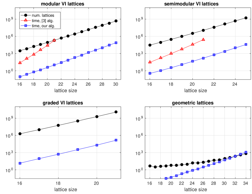
Figure 3. Number of vertically indecomposable lattices by size, and running times of two algorithms ([5] and ours). All times are in seconds on a single 2.6 GHz Intel Xeon E5-2690 core.

We do not have theoretical guarantees on the running time of our algorithm, but some empirical observations can be made. Fig. 3 illustrates the number of lattices and the time spent by our algorithm. Both exhibit somewhat similar scaling with respect to lattice size, indicating that the algorithm is doing a reasonable job in finding the relevant portions of the search space (except for geometric lattices). Let us inspect in more detail the numerical growth ratios between consecutive lattice sizes.

Modular vi-lattices. Between sizes $n=27$, $28$, $29$, $30$, the number of vertically indecomposable modular lattices grows by ratios $2.38$, $2.38$, $2.39$ (see Table 1), suggesting a rather stable exponential growth. For the same sizes our running time grows by ratios $2.68$, $2.75$, $2.74$. So empirically the growth rate is slightly below ${2.4}^{n}$ for number of lattices and ${2.8}^{n}$ for running time. This is not quite ideal: the gap of about $0.4$ between the bases of the exponents raises the question whether one could construct an output-sensitive algorithm to generate modular lattices, that is, one whose running time is linear in the size of the output.

Semimodular vi-lattices. Across sizes $n=22$, $23$, $24$, $25$, the number of lattices grows roughly as ${3.6}^{n}$ and our running time as ${4.0}^{n}$, again with a gap of $0.4$ between the bases.

Graded vi-lattices. Across sizes $n=18$, $19$, $20$, $21$, the number of lattices grows by ratios $5.74$, $5.93$, $6.13$, exhibiting faster than exponential growth. The running time grows by ratios $6.38$, $6.16$ and $7.03$, again somewhat faster than the number of lattices.

Geometric lattices. The number of geometric lattices grows so slowly that no asymptotic form is discernible from the available numbers. The running time grows much faster than the number of lattices.

To compare the performance, we reran Jipsen and Lawless’s program [5] for modular and semimodular vi-lattices, both up to size 21. These running times are shown in Fig. 3 with red triangles. Between sizes $n=18$, $19$, $20$, $21$, the running time for modular vi-lattices grew by ratios $5.90$, $6.27$, $6.81$, with $n=21$ taking $2.1$ days of processor time. From this we estimate that $n=24$ would have required about two years of processor time (about $300\;000$ times more than with our algorithm, which completed in 194 seconds).

We conclude this section with some remarks on the speed of our basic algorithm for generating graded lattices. At size $n=21$ it outputs about $82\;000$ graded lattices per second, or one lattice in $12$ microseconds. On the 2.6 GHz processor that was used, this amounts to $32\;000$ clock cycles per lattice. Gebhardt and Tawn [3] count general (not graded) lattices considerably faster, at $2\;200$ clock cycles per lattice. They handle isomorphisms with a sophisticated method specially tailored to lattices. In contrast, our algorithm handles only the simplest cases directly, and in more complicated cases resorts to using the general-purpose graph isomorphism tool nauty as a “black box”. Indeed, during the search for graded 21-lattices, our algorithm performs about $2.7\times 10^{10}$ calls to nauty. Taking $3.4$ microseconds per call on average, together they account for 65% of the total running time. While Gebhardt and Tawn considered general lattices only, it might be useful to combine their method for isomorphisms with our early checks for (semi)modularity.

8. Results

The lattice listings are available for download [7, 8, 9]. The numbers of lattices are shown in Tables 1 and 2. Vertically indecomposable modular, semimodular and graded lattices were directly counted by the program; numbers that include decomposable lattices were then calculated with the recursion formula [4]

$$u(n)=\sum_{k=2}^{n}u_{\text{vi}}(k)\;u(n\!-\!k\!+\!1),\qquad\text{for $n\geq 2$},$$

where $u(n)$ counts all unlabeled lattices of size $n$ in the relevant family, and $u_{\text{vi}}(n)$ counts vi-lattices only. For geometric lattices the recursion formula does not apply as they are necessarily vertically indecomposable.

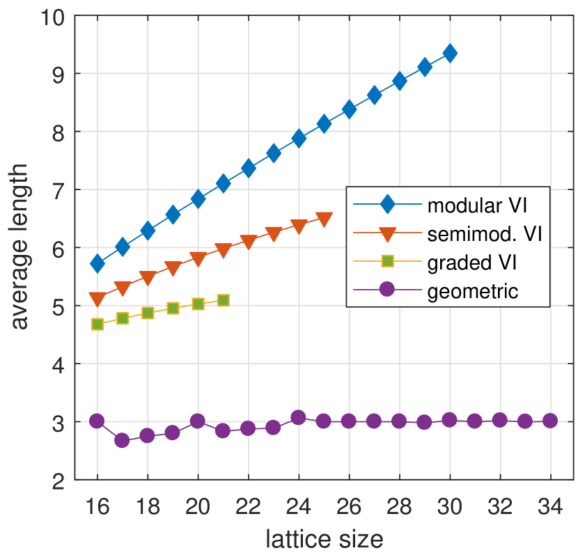
Figure 4. Average lattice length as a function of lattice size.

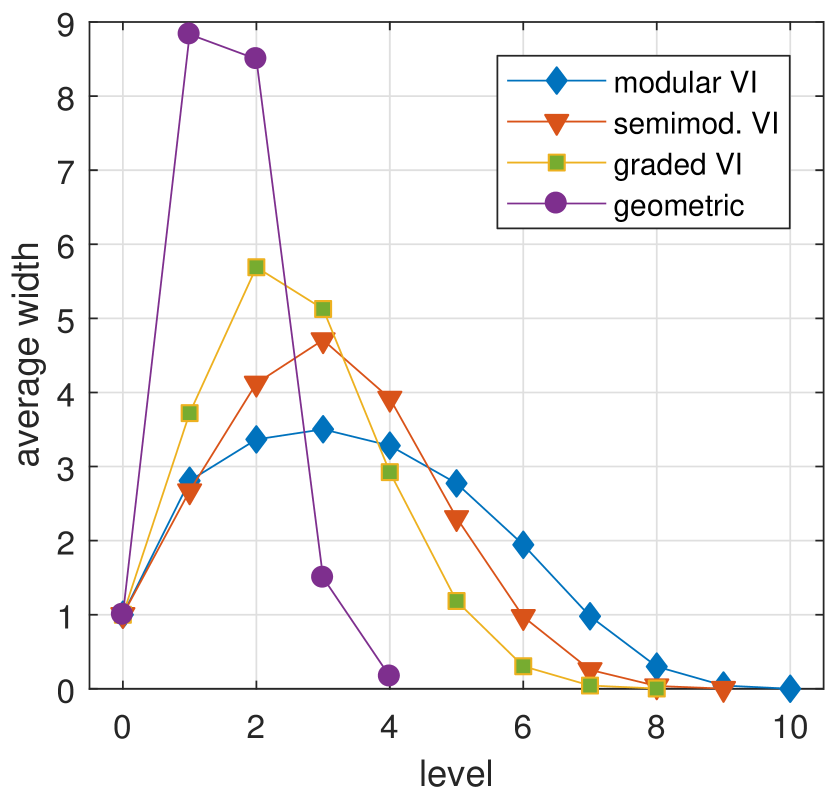
Figure 5. Average widths (numbers of elements) of levels in lattices of size 21.

The numbers seem to suggest exponential growth of modular and semimodular lattices; indeed, Jipsen and Lawless [5] have proven a lower bound of the form $\mathrm{\Omega}(2^{n})$ for the number of modular lattices. This raises the question of finding an upper bound $O(c^{n})$ with some constant $c$. To the best of our knowledge, no such upper bound is known for modular or semimodular lattices. In contrast, it is known that the number of graded lattices grows faster than exponentially in $n$ [6].

Apart from total numbers, one may compute various statistics from the actual lattice listings. As an example, from Figs. 5 and 5 we observe that typical lattices in these four families have quite different length and width characteristics: modular lattices are long and narrow while geometric lattices are short and wide. Semimodular and graded lattices are in between. Empirical understanding of the typical lattice shape may be useful, for example, when formulating hypotheses about asymptotics, and in algorithm design.

$n$		modular vi	modular			semimodular vi	semimodular
1		1	1			1	1
2		1	1			1	1
3		0	1			0	1
4		1	2			1	2
5		1	4			1	4
6		2	8			2	8
7		3	16			4	17
8		7	34			9	38
9		12	72			21	88
10		28	157			53	212
11		54	343			139	530
12		127	766			384	1 376
13		266	1 718			1 088	3 693
14		614	3 899			3 186	10 232
15		1 356	8 898			9 596	29 231
16		3 134	20 475			29 601	85 906
17		7 091	47 321			93 462	259 291
18		16 482	110 024			301 265	802 308
19		37 929	256 791			990 083	2 540 635
20		88 622	601 991			3 312 563	8 220 218
21		206 295	1 415 768			11 270 507	27 134 483
22		484 445	3 340 847			38 955 164	91 258 141
23		1 136 897	7 904 700			136 660 780	312 324 027
24		2 682 451∗	18 752 943∗			486 223 384	1 086 545 705
25		6 333 249	44 588 803			1 753 185 150	3 838 581 926
26		15 005 945	106 247 120
27		35 595 805	253 644 319
28		84 649 515	606 603 025
29		201 560 350	1 453 029 516
30		480 845 007	3 485 707 007

Table 1. Numbers of unlabeled modular and semimodular lattices by size (vi = vertically indecomposable). New numbers are highlighted; corrections to previous numbers marked with ^∗.

$n$		graded vi	graded			geometric
1		1	1			1
2		1	1			1
3		0	1			0
4		1	2			1
5		1	4			1
6		3	9			1
7		7	22			1
8		22	60			2
9		68	176			1
10		242	565			2
11		924	1 980			1
12		3 793	7 528			3
13		16 569	30 843			2
14		76 638	135 248			2
15		372 838	630 004			3
16		1 900 132	3 097 780			5
17		10 105 175	15 991 395			3
18		55 895 571	86 267 557			4
19		320 655 822	484 446 620			5
20		1 903 047 753	2 822 677 523			6
21		11 658 925 558	17 017 165 987			6
22						8
23						9
24						16
25						16
26						21
27						29
28						45
29						50
30						95
31						136
32						220
33						392
34						680

Table 2. Numbers of unlabeled graded and geometric lattices by size (vi = vertically indecomposable). New numbers are highlighted.

9. Conclusion

Let us conclude with some thoughts of future research. Based on the empirical running times and memory usage, it seems quite feasible to count modular lattices a little further with our program as it is: modular $32$-lattices might be counted in about one week of processor time, requiring a few gigabytes of memory to keep the daughter lattice lists for isomorph rejection. The computation can be parallelized by running a separate job for each initial lattice $M_{j}$. Extending the counts of semimodular lattices seems also feasible.

However, it might be more interesting to pursue other methods of counting modular lattices, possibly without explicitly generating them. Jipsen and Lawless [5] discuss some prospects of using alternative representations of modular lattices to count them. Another prospect comes from our observation that modular lattices tend to be long and narrow: perhaps a large portion of modular lattices could be counted implicitly, by considering some kind of vertical compositions of smaller modular lattices, without explicitly listing the compositions.

For counting graded lattices, the current program does not seem well suited to larger sizes. Compared to modular lattices, graded lattices tend to be shorter and wider, which becomes a problem in our method of isomorph rejection: a single mother lattice may have a large number of daughter lattices, so the memory required for storing the daughters becomes excessive. It would seem necessary to improve the isomorph rejection method so as to use less memory.

Geometric lattices share the problem of being short and wide. Another problem is that our current method generates a large number of lower semimodular proposals, then rejects the vast majority of them for not being co-atomistic. This seems very inefficient, and better methods would be desirable, for example, ones that would reject the proposed lattices earlier.

References

- [1] Gunnar Brinkmann and Brendan D. McKay. Posets on up to 16 points. Order, 19(2):147–179, 2002.
- [2] Marcel Erné, Jobst Heitzig, and Jürgen Reinhold. On the number of distributive lattices. The Electronic Journal of Combinatorics, 9(1):#R24, 2002.
- [3] Volker Gebhardt and Stephen Tawn. Constructing unlabelled lattices. ArXiv e-prints, September 2016.
- [4] Jobst Heitzig and Jürgen Reinhold. Counting finite lattices. Algebra universalis, 48(1):43–53, 2002.
- [5] Peter Jipsen and Nathan Lawless. Generating all finite modular lattices of a given size. Algebra universalis, 74(3):253–264, 2015.
- [6] D. J. Kleitman and K. J. Winston. The asymptotic number of lattices. Ann. Discrete Math., 6:243–249, 1980.
- [7] Jukka Kohonen. Lists of finite lattices (graded, n=21 elements, c=2 coatoms). https://b2share.eudat.eu/records/dda62689eb724e9ea6a40b9cd280cfed.
- [8] Jukka Kohonen. Lists of finite lattices (graded, n=21 elements, c2 coatoms). https://b2share.eudat.eu/records/9fa46c3cc366477cb3894ea14a83f7de.
- [9] Jukka Kohonen. Lists of finite lattices (modular, semimodular, graded and geometric). https://b2share.eudat.eu/records/dbb096da4e364b5e9e37b982431f41de.
- [10] Martin Malandro. The unlabeled lattices on 15 nodes. http://www.shsu.edu/mem037/Lattices.html, 2013.
- [11] Brendan D. McKay and Adolfo Piperno. Practical graph isomorphism, II. Journal of Symbolic Computation, 60:94–112, 2014.
- [12] Brendan D. McKay and Adolfo Piperno. Nauty and Traces User’s Guide (Version 2.6). http://pallini.di.uniroma1.it/Guide.html, 2016.
- [13] Neil J. A. Sloane. The On-line Encyclopedia of Integer Sequences. https://oeis.org.
- [14] Richard P. Stanley. Enumerative Combinatorics, volume 1. Wadsworth & Brooks, Belmont CA, 1986.