Generalized Graph Pattern Matching

1 Introduction

Graphs are high expressive models and especially suitable for modelling highly complex structures, the number of applications that use them for modelling both their data and the processes that manipulate has grown dramatically in recent years.

The use of new conceptual structures in real-world applications requires the development of new systems to store and query such structures in order to allow users to access data effectively and efficiently. As with all new technologies, it is still in the development phase and in search of a set of standards ensuring a continued growth.

The growing popularity of Graph Databases has led to the emergence of interesting problems related to storage and query in these systems. These databases have robust fundamentals in terms of basic information management (creation, access, deletion, and modification of individual elements of the structure), but they lack standards in some other tasks necessary for the storage and retrieval of information, like those related to more advanced query mechanisms.

Among the problems related to these query processes, the detection of patterns is considered as one of the fundamental ones since it includes other subproblems necessary to obtain powerful query systems, such as the search of subgraphs or minimum paths, or the study of connectivity [18, 10].

In this paper we present Generalized Graph Query (GGQ), a proposal to carry out queries in property graphs. GGQ represents a robust logical framework, making it especially useful in graph discovery procedures and generalizing other more basic tools that have been proved very useful on related tasks. In addition, we will present a collection of operations that allow to obtain complex GGQs from simpler ones, something very useful when automating the construction of complex queries.

2 Graph Pattern Matching

Graph Pattern Matching is an active research area since more than 30 years and its usefulness has been demonstrated in many areas, from artificial vision, to biology, through electronics, computer-aided design, and analysis of social networks, among others. Undoubtedly, its interest has grown even more as graph databases has become a tool for structuring and storing information in a transversal way in all areas of knowledge. For this reason, the problem of graph pattern matching expands, with slight variants, across different scientific communities, showing that is not a single problem defined under a common formalization, but a set of related problems.

The process by which we check the presence of a particular pattern in a particular set of data is called pattern detection, and computationally represents the set of mechanical processes that allow to return one (or all) the occurrences of the pattern.

The definition of what is meant by an occurrence of a pattern in a graph varies according to how the pattern is defined. When it is given by a graph structure (although not necessarily using the same elementary sets of vertices and edges as the graph on which the query is made) it is usual to associate the occurrence with the existence of identifications (perhaps not as strong as isomorphisms) between the pattern and those subgraphs in the data that respect some imposed constraints [6].

Some classifications that we can present in terms of the different possible ways to carry out the detection of patterns in graphs are: (a) Structural vs. Semantic, (b) Exact vs. Inexact, and (c) Optimal vs. Aproximate [9].

One other classification takes into account the relation to be met by the pattern regarding to the subgraphs that are considered its occurrences. It allows to divide the different techniques of graph pattern matching in those based on Isomorphisms (an occurrence will be any subgraph that is isomorphic to the pattern), Graph Simulation [13] (an occurrence will be any subgraph for which there is a binary relation between the elements of the subgraph and the pattern which respects the types of the nodes and their adjacencies), Bounded Simulation [8, 18, 13] (based on Graph Simulation but allowing to associate pattern edges to paths) and Regular Pattern Matching [7, 15, 4, 13] (Bounded Simulation with regular expressions for pattern edges).

Current tools that allow querying patterns in graphs use either a declarative language (such as Cypher, SPARQL, or SQL), or an imperative language (with Gremlin as the clearest representative). In the case of declarative languages, it is responsibility of the system (ideally) to perform queries optimization. In the case of imperative languages, the execution plan is responsibility of the user, so they usually provide lower level approximations.

Next, we briefly present some query languages that have been used for graph pattern matching.

SQL (Structured Query Language) is a declarative language for accessing Relational Database Management Systems (RDBMS). These types of databases were designed for tabular data with a fixed schema, and work best in contexts that are well defined from the beginning and where the records themselves are more important than the relationships between them. For this reason, trying to answer questions involving many relationships between data (as is usual in graph pattern queries) with a relational database involves numerous and costly operations between tables, that may become this option intractable. In spite of this, SQL has the expressive capacity necessary to be able to express most of graph pattern queries, and because relational databases have been the storage option chosen by most projects for decades, the first graph pattern query systems used SQL queries, such as Selection Graphs that we will see later.

SPARQL is a declarative query language for data stored in RDF format [16] and is recognized as a key technology of the Semantic Web, its expressive ability to perform graph pattern matching is superior to that provided by SQL, but is still not intuitive for a human user. SPARQL allows structural, semantic, optimal, and exact queries based on subgraph isomorphism. Although SPARQL does not allow for any type of Graph Simulation or Regular Pattern Matching, language extensions such as PSPARQL [3] have been developed to query RDF databases using patterns that make use of regular expressions. Thanks to the structure of the language, it is relatively easy to generate automatic queries in SPARQL and there are tools that use it as a final query language.

Gremlin is, at the same time, a query language for databases and a graph oriented computation system. As a language, Gremlin is independent of the underlying database. Its syntax allows for declarative and imperative queries, and easily express complex queries on graphs. Each query consists of a sequence of steps that perform atomic operations on the data stream. Gremlin allows semantic, exact, optimal queries and is based on subgraph isomorphism. It is possible to design other query languages to compile to Gremlin language (eg, SPARQL can be compiled to run on Gremlin ).

Selection Graphs are multi-relational patterns to express SQL based queries. They represent the foundation of the multi-relational decision tree induction algorithm MRDTL [12] as well as other multi-relational automatic learning algorithms [14]. The purpose of selection graphs is to be used in top-down discovery procedures [11], thus operators to modify them through small changes are provided that allow the construction of complex queries in successive steps. As a counterpart, they have the disadvantage that these constructions can not contain cycles, limiting the expressiveness of queries. Selection graphs represent an exact, optimal type of graph pattern matching based on semantic graph isomorphism. In addition, being a graphical representation of SQL queries, they inherit the efficiency problems presented by the systems based on this technology. The new proposal we show in these pages can be considered as a generalization of some of the ideas that promoted this previous approach, avoiding some of their limitations.

Cypher is a declarative query language specifically developed to work on Neo4j graph database . Cypher is designed to be a human-friendly query language, close to both developers and end users. Query patterns in graphs that are usually hard to express in other languages are very simple in Cypher [2], showing a high expressive capacity [1]. Neo4j database closely follows the property graph model, but forces the edges to be typed. Unlike Gremlin, Cypher is not Turing complete, so it has some limitations, and it is higher level. Simple Cypher queries have good performance, but when queries follow complex patterns they can lead to a worst performance since it does not allow to indicate the application order of the different conditions. Cypher allows structural and semantic, optimal, exact, and based on subgraph isomorphism queries. In addition, it allows a type of Regular Pattern Matching in which the edges in the pattern are projected onto paths of the graph, and where constraints can be imposed through expressions that make use of the disjunction operator and the closure of Kleene. One limitation from the academic point of view is that it lacks an associated formal model, and some of its operations have not yet been validated. Despite this, because of its excellent expressiveness and acceptable performance, and because it consumes the data from a graph database with a widespread use, Cypher has been the election to implement the tests of GGQ.

Some other tools related to graph pattern matching are: GraphLog [5], that allows to structure the queries as graphs and evaluates the existence of patterns between a pair of nodes to generate a new edge between them; GraphQL , a declarative query language developed by Facebook to allow external applications to access its information; Graql , a declarative query language oriented to knowledge graphs; and GGQL [17], a SQL extension with additional graph pattern matching tools (analysis of accessibility between nodes, definition of paths, or construction of graphs).

3 Preliminaries

Given a set $V$, we denote:

$$V^{0}=\emptyset,\ V^{1}=V,\ V^{n+1}=V^{n}\times V,\ V^{*}=\bigcup_{n\geq 0}V^{n}$$

In general, we call sequences or lists the elements in $V^{*}$. If $x\in V^{n}$ then we say that $x$ has length $n$, and we write $|x|=n$.

If $x=(a_{1},\dots,a_{n}),y=(b_{1},\dots,b_{m})\in V^{*}$, then the concatenation of $x$ and $y$ is the element of $V^{*}$ given by $xy=(a_{1},\dots,a_{n},b_{1},\dots,b_{m})$.

For each $x=(a_{1},\dots,a_{n})\in V^{n}$, we call support set of $x$ to $s(x)=\{a_{i}:1\leq i\leq n\}$. We write $a\in x$ to indicate that $a\in s(x)$.

For each $a\in V$, we denote $|a|_{x}=\#\{i:x_{i}=a\}$ (where $\#(A)$ is the cardinal of the set $A$), and we call multi-support of $x$ to the set of pairs $ms(x)=\{(a,|a|_{x}):a\in x\}$. We define the relation $\sim$, which can be easily proved to be equivalence in $V^{n}$, as: $x\sim y$ if and only if $ms(x)=ms(y)$ And denote by $V_{\sim}^{n}=V^{n}/\sim$ (set quotient of $V^{n}$ under $\sim$).

Our interpretation of these sets will be that $V^{n}$ denotes the set of ordered tuples of $V$, $V_{\sim}^{n}$ denotes the set of unordered tuples of the same set (ie tuples in which elements are important, considering the possible repetitions, but not the order in which they appear).

Next, we present the Generalized Graph, that covers the different variants of graph that can be found in the literature and that we will need when presenting our proposal of property graph pattern matching tool.

Definition 1.

A Generalized Graph is a tuple $G=(V,E,\mu)$ where:

• $V$ and $E$ are sets, called, respectively, set of nodes and set of edges of $G$.

• $\mu$ is a relation (usually we will consider it functional, but not necessarily) that associates each node or edge in the graph with its set of properties, that is, $\mu:(V\cup E)\times R\rightarrow S$, where $R$ represents the set of possible keys for these properties, and $S$ the set of possible values associated.

Usually, for each $\alpha\in R$ and $x\in V\cup E$, we write $\alpha(x)=\mu(x,\alpha)$.

In addition, we require the existence of a special key for the edges of the graph, which we call incidences and denote by $\gamma$, which associates to each edge of the graph a tuple, ordered or not, of vertices of the graph.

Although the definition that we have presented here is more general than those that can be found in the related literature, we will also call them Property Graphs, since they suppose a natural extension of this type of graphs.

It should be noted that in generalized graphs, unlike traditional definitions, the elements in $E$ are symbols representing the edges, and not pairs of elements from $V$, and $\gamma$ is the function that associates to each edge the set of vertices that it connects.

Definition 2 (Notation and definitions).

In the context of the above definitions, we use the following notation:

• We usually identify $e$ with $\gamma(e)$. Thus, we interpret the edge as the collection of nodes that connects, as classic definitions of graphs.

• Symmetrically, for every $u\in V$ we write $\gamma(u)=\{e\in E:u\in e\}$. In general, a generalized graph may have a combination of directed and non-directed edges. If $\gamma:E\rightarrow V^{*}$ we say $G$ to be Directed (Not Directed, otherwise).

• For each $e\in E$, we define the arity of $e$ as $\sum_{a\in e}|a|_{e}$.

• If $\gamma:E\rightarrow V^{2}\cup V_{\sim}^{2}$ we say that the graph is Binary (and it matches the most usual graph structure). Otherwise, the graph is a Hypergraph.

• An edge, $e\in E$, is said to be a loop if it connects a node to itself, that is, if it has arity other than 1 but $s(e)$ is unitary.

• An edge, $e\in E$, is said to be incident on a node, $v\in V$, if $v\in e$.

• Two distinct nodes, $u,v\in V$ are called adjacent, or neighbors, in $G=(V,E,\mu)$ if there exists $e\in E$ such that $\{u,v\}\subseteq e$.

• If there are different edges in $E$ with the same incidence, that is, edges connecting the same nodes, we will say that the graph is a Multi-graph.

• If $e$ is a directed binary edge connecting $u$ to $v$, $e=(u,v)$, we write $u\overset{e}{\rightarrow}v$, and we also denote $e^{o}=u$ (output of $e$) y $e^{i}=v$ (input of $e$). In this case, for each $u\in V$ we write:

  $$\gamma^{o}(u)=\{e\in\gamma(u):\ e^{o}=u\}$$

  $$\gamma^{i}(u)=\{e\in\gamma(u):\ e^{i}=u\}$$

  which respectively denote the sets of outgoing edges and incoming edges of $u$.

• Given $u\in V$, we define the environment of $u$ in $G$ as the set of nodes, including $u$, that are connected to it, i.e.: $\mathcal{N}(u)=\bigcup_{e\in\gamma(u)}\gamma(e)$. When necessary, we will use the reduced environment of $u$, $\mathcal{N}^{*}(u)=\mathcal{N}(u)\setminus u$.

The notion of subgraph is obtained from the usual definition by imposing that the properties are also maintained in the common elements.

Definition 3.

A subgraph of a graph $G=(V,E,\mu)$ is a graph $S=(V_{S},E_{S},\mu_{S})$ such that $V_{S}\subseteq V$ and $E_{S}\subseteq E$ and $\mu_{S}\subseteq\mu_{|V_{S}\cup E_{S}}$. We denote $S\subseteq G$.

A fundamental concept when working with graphs is the concept of path, which allows the study of distance relationships and connectivity conditions between different elements, extending the connectivity allowed by edges to more general situations.

As generalized graphs are considerably more general than the usual ones we should give some notions about the position of a node in an edge:

Definition 4.

If $e\in E$ and $\gamma(e)=(v_{1},\dots,v_{n})\in V^{n}$, then for each $v_{i}\in s(e)$ we define its order in $e$ as $ord_{e}(v_{i})=i$. If $e\in V_{\sim}^{n}$, then for each $v\in s(e)$ we define $ord_{e}(v)=0$.

We denote $u\leq_{e}v$ to indicate that $ord_{e}(u)\leq ord_{e}(v)$.

From this relation of order between the nodes that an edge connects, we can define what we mean by a path in a graph.

Definition 5.

Given a graph $G=(V,E,\mu)$, the set of paths in $G$, denoted by $\mathcal{P}_{G}$, is defined as the minimal set verifying:

1. If $e\in E$, $u,\ v\in e$ with $u\leq_{e}v$, then $\rho=u\overset{e}{\rightarrow}v\in\mathcal{P}_{G}$, and $sop_{V}(\rho)=(u,v)$, $sop_{E}(\rho)=(e)$. We will say that $\rho$ connects the nodes $u$ and $v$ of $G$, and we will denote it by $u\overset{\rho}{\rightsquigarrow}v$.

2. If $\rho_{1},\ \rho_{2}\in\mathcal{P}_{G}$, with $u\overset{\rho_{1}}{\rightsquigarrow}v,\ v\overset{\rho_{2}}{\rightsquigarrow}w$, then $\rho_{1}\cdot\rho_{2}\in\mathcal{P}_{G}$, with $u\overset{\rho_{1}\cdot\rho_{2}}{\rightsquigarrow}w$, $sop_{V}(\rho_{1}\cdot\rho_{2})=sop_{V}(\rho_{1})sop_{V}(\rho_{2})$, $sop_{E}(\rho_{1}\cdot\rho_{2})=sop_{E}(\rho_{1})sop_{E}(\rho_{2})$.

When $u=v$ we say that $\rho$ is a closed path, and if there are not repeated edges in $\rho$ we say that it is a cycle.

If $\rho\in\mathcal{P}_{G}$, with $sop_{V}(\rho)=(u_{1},\dots,u_{n+1})$ and $sop_{E}(\rho)=(e_{1}\dots,e_{n})$, then we write:

$$\rho=u_{1}\overset{e_{1}}{\rightarrow}u_{2}\overset{e_{2}}{\rightarrow}\dots\overset{e_{n}}{\rightarrow}u_{n+1}$$

Generally we will write $u\in\rho$ to express that $u\in sop_{V}(\rho)$, and $e\in\rho$ to express that $e\in sop_{E}(\rho)$.

Remark.

• Following a similar notation to the case of directed binary edges, if $\rho\in\mathcal{P}(G)$ and $u\overset{\rho}{\rightsquigarrow}v$, then we write $\rho^{o}=u$ and $\rho^{i}=v$.

• When necessary, we denote the paths through $u$, starting in $u$, and ending in $u$, respectively, by:

  $$\mathcal{P}_{u}(G)=\{\rho\in\mathcal{P}(G):\ u\in\rho\}$$

  $$\mathcal{P}_{u}^{o}(G)=\{\rho\in\mathcal{P}(G):\ \rho^{o}=u\}$$

  $$\mathcal{P}_{u}^{i}(G)=\{\rho\in\mathcal{P}(G):\ \rho^{i}=u\}$$

4 Generalized Graph Query

Next, we present Generalized Graph Query (GGQ, for short), our proposal to perform graph pattern matching on generalized graphs. Taking into account the different classifications mentioned above, we can say that this proposal allows to carry out structural and semantic, exact, optimal, and based on a type of Regular Pattern Matching queries, allowing the edges of the pattern to be projected on paths (not necessarily edges). Also, GGQ allows to express more complex constraints on each element of the pattern and perform cyclic queries.

One of the characteristics that we pursue for our tool is to provide a mechanism to obtain complementary patterns to a given one. This means that if a structure does not verify a pattern it must always verify one of its complementary patterns. As we have seen in previous section, many of the tools developed to perform queries of patterns in graphs require for a projection to be fulfilled between the pattern and the structure to be evaluated. This projection prevents us from evaluating the non existence of elements, something that we will need to generate these complementary patterns, for this reason our proposed matching system will not make use of projections, but is based on logical predicates, facilitating the generation of complementary patterns.

We want to emphasize that one of our main goals is to provide a complete formalization of the model, but with the secondary objective of providing an implementation that is usable from a practical point of view (as a proof of concept more than as a professional tool in this first stage).

In pursuit of our objectives, we will rely on Selection Graph model, extending it to add Regular Pattern Matching and some additional features that will allow us to obtain a greater expressiveness power in the patterns.

As main differences with the query systems from the previous section we can indicate that:

• GGQ may contain cycles. It will be a later problem to consider implementations of GGQs that handle cycles properly, considering additional constraints to ensure certain levels of efficiency in their actual execution, or being careful when designing the query to create a pattern that is efficient in the available implementation.

• GGQ can evaluate subgraphs. In selection graphs it is only possible to evaluate a single node representing the target table. In the case of GGQ, fixed elements (elements that must belong to the subgraph under evaluation) will be represented through a predicate that forces them to be contained in the subgraph to be evaluated.

• Individual edges of the GGQ can be projected onto paths in the graph where the pattern is being checked. For this reason, predicates will be used in a similar way as in Regular Pattern Matching.

• The predicates associated with nodes or edges in the GGQ can evaluate structural and semantic characteristics beyond the properties stored through the $\mu$ function (for example, using metrics on the graph or its elements).

We will briefly formalize what we understand concretely by a predicate defined on a graph.

Consider $\Theta$, a collection of function, predicate, and constant symbols, containing all the functions from $\mu$ together with constants associated with each element of the graph and possibly some additional symbols (for example, metrics defined on the elements of the graph). From this set of symbols we can define a First Order Language with equality, $L$, making use of $\Theta$ as a set of non logical symbols, on which we construct, in the usual way, the set of terms of the language and the set of formulas, $FORM(L)$, which we will call predicates.

Although, generally, the definable formulas in $L$ can be applied to all objects in the universe, which in our context will consist in elements of graphs (nodes, edges, and structures formed from them), when we want to make explicit the types of objects we are working with, we can write $FORM_{V}(L)$ for formulas on nodes, $FORM_{E}(L)$ for formulas on edges, $FORM_{\mathcal{P}}(L)$ for formulas on paths, etc.

In order to simplify the notation, when there is no possibility of confusion we will use $FORM$ to denote $FORM(L)$.

In addition, and taking advantage of the expressiveness capacity of generalized graphs, we define the query system using the same structure:

Definition 6.

A Generalized Graph Query (GGQ) over $L$ is a binary generalized graph, $Q=(V_{Q},E_{Q},\mu_{Q})$, where exist $\alpha$ and $\theta$, properties in $\mu_{Q}$, such that:

• $\alpha:V_{Q}\cup E_{Q}\rightarrow\{+,-\}$ total.

• $\theta:V_{Q}\cup E_{Q}\rightarrow FORM(L)$ associates a binary predicate, $\theta_{x}$, to each element $x$ of $V_{Q}\cup E_{Q}$.

We will write $Q\in GGQ(L)$ to denote that $Q$ is a Generalized Graph Query over $L$ (if the language is prefixed, we simply write $Q\in GGQ$).

In the semantics associated with a GGQ we will use the second input of these binary predicates to impose requirements of membership on subgraphs of $G$ (the general graph on which we are evaluating queries), whereas the first input must receive elements of the corresponding type to which it is associated: if $S$ is a subgraph and $a\in V_{Q}$ then $\theta_{a}(.,S)\in FORM_{V}$, and if $e\in E_{Q}$ then $\theta_{e}(.,S)\in FORM_{\mathcal{P}}$. For example:

$$\theta_{a}(v,S) =\exists z\in S\ (z\overset{}{\rightsquigarrow}v)$$

$$\theta_{e}(\rho,S) =\exists y,z(y\overset{\rho}{\rightsquigarrow}z\wedge y\notin S\wedge z\in S)$$

$\theta_{a}(v,S)$ will work for nodes, and it will be verified when there is a path in $G$ that connects a node of $S$ (the subgraph we are evaluating) with $v$, the input node on which it is evaluated. $\theta_{e}(\rho,S)$ will work for paths, and will be verified when the evaluated path, $\rho$, connects $S$ with its complementary (in $G$).

Given a GGQ under the above conditions, $x^{+}$, respectively $x^{-}$, will indicate that $\alpha(x)=+$, respectively $\alpha(x)=-$, and $V_{Q}^{+}/V_{Q}^{-}$ (respectively, $E_{Q}^{+}/E_{Q}^{-}$) the set of positive/negative nodes (respectively, edges). If for an element, $\theta_{x}$ is not explicitly defined, we assume it to be a tautology (generally denoted by $T$).

As we will see below, positive elements of the pattern represent elements verifying the associated predicates that must be present in the graph, while negative ones represent elements that should not be present in the graph.

In order to be able to express more easily the necessary conditions that define the application of a GGQ on a graph, as well as the results that we will see later, we introduce the following notations:

Definition 7.

Given a GGQ, $Q=(V_{Q},E_{Q},\mu_{Q})$, the set of $Q$-predicates associated to $Q$ is:

1. For each edge, $e\in E_{Q}$, we define:

   $$Q_{e^{o}}(v,S)=\exists\rho\in\mathcal{P}_{v}^{o}(G)\ \left(\theta_{e}(\rho,S)\wedge\theta_{e^{o}}(\rho^{o},S)\wedge\theta_{e^{i}}(\rho^{i},S)\right)$$

   $$Q_{e^{i}}(v,S)=\exists\rho\in\mathcal{P}_{v}^{i}(G)\ \left(\theta_{e}(\rho,S)\wedge\theta_{e^{o}}(\rho^{o},S)\wedge\theta_{e^{i}}(\rho^{i},S)\right)$$

   In general, we will write $Q_{e^{*}}(v,S)$, where $*\in\{o,i\}$, and we will denote:

   $$Q_{e^{*}}^{+}=Q_{e^{*}},\hskip 28.45274ptQ_{e^{*}}^{-}=\neg Q_{e^{*}}$$

2. For each node, $n\in V_{Q}$, we define:

   $$Q_{n}(S) =\exists v\in V\ \left(\bigwedge_{e\in\gamma^{o}(n)}Q_{e^{o}}^{\alpha(e)}(v,S)\ \wedge\bigwedge_{e\in\gamma^{i}(n)}Q_{e^{i}}^{\alpha(e)}(v,S)\right)$$

   $$=\exists v\in V\ \left(\bigwedge_{e\in\gamma^{*}(n)}Q_{e^{*}}^{\alpha(e)}(v,S)\right)$$

   That can be written generally as:

   $$Q_{n}(S)=\exists v\in V\ \left(\bigwedge_{e\in\gamma(n)}Q_{e}^{\alpha(e)}(v,S)\right)$$

   In addition, we denote:

   $$Q_{n}^{+}=Q_{n},\hskip 28.45274ptQ_{n}^{-}=\neg Q_{n}$$

From these notations, we can formally define when a subgraph matches a given GGQ:

Definition 8.

Given a subgraph $S$ of a property graph, $G=(V,E,\mu)$, and a Generalized Graph Query, $Q=(V_{Q},E_{Q},\mu_{Q})$, both over language $L$, we say that $S$ matches $Q$, and we will denote $S\vDash Q$, if the next formula is verified:

$$Q(S)=\bigwedge_{n\in V_{Q}}Q_{n}^{\alpha(n)}(S)$$

Otherwise, we will write: $S\nvDash Q$.

Note that, in particular, using $S=G$ we can define when a graph matches a GGQ. A generic GGQ example is shown in Figure 1.

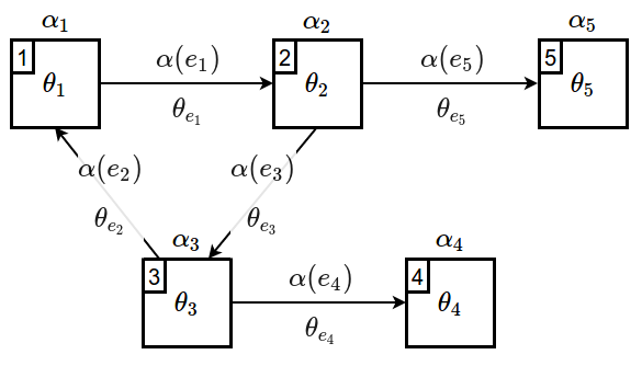
Figure 1: Generalized Graph Query Example.

One of the objectives for GGQ is to provide power enough to express conditions that make use of elements that are outside the subgraph being evaluated, something that has been proven necessary to have a powerful query language and, except in the selection graphs (and only to a very limited extent), it is not present in the other previous solutions.

Although the definition of GGQ makes use of binary graphs (not hypergraphs), since it projects edges on paths connecting pairs of nodes, the generalized graph concept is flexible enough to allow other interpretations where GGQ can use more general structures. In addition, and it is important to emphasize this fact, although GGQ are binary graphs, they can be applied on hypergraphs with properties, since the concept of path that connects pairs of nodes is defined independently of the arity of the intervening edges. In these cases, a somewhat more complex notation should be used to define the $Q$-predicates, but it is completely feasible. For the sake of simplicity, and because of the lack of hypergraph databases, we have restricted the definitions to these particular cases, but they are open to be extended to more general cases at the moment in which the use of hypergraphs is generalized as tools of modelling and storage, since in most of the (rare) occasions they have been needed, the problem has always been solved by means of the creation of new types of nodes and binary edges that simulate the presence of hyperlinks.

Before going on to analyse some interesting properties about GGQ and how to construct them, let’s see some examples that allow us to understand how they are interpreted and the expressive capacity they allow.

5 Some Representative Examples

Figure 2 shows a property graph that corresponds to a section of a graph database that contains information about the main characters of the Starwars series and that is frequently used as a simple example to do demonstrations related to graph database capabilities . We will use this graph to present some GGQ examples and to check the verification of some specific subgraphs.

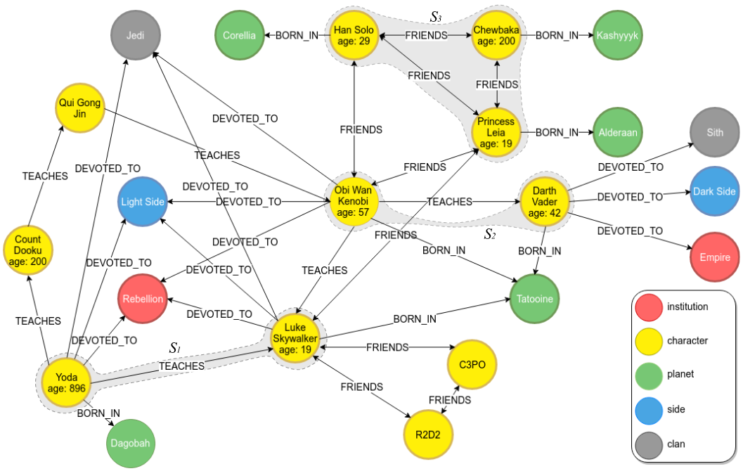
Figure 2: Starwars graph to present some Generalized Graph Query examples.

In order to simplify the representation of queries and subgraphs, one of the properties in $\mu$, which we will call $\tau$ and which represents types on nodes and edges, will be expressed directly on the edges and, in the case of nodes, through colours. In addition, the name property of the nodes will be represented directly on them, and the undirected edges will be represented as bidirectional edges.

The graphical representation of the example GGQs are shown in figures 3 to 8. When analysing the interpretation of these queries we will also indicate some subgraphs of $G$ verifying them. The $\alpha$ property will be directly represented on the elements of GGQ by means of a $+/-$ symbol, and $\theta$ property directly in the element (but in the case of tautologies). In expressions of the type $\tau(\rho)=X$ in the predicate of an edge, $X$ is interpreted as a regular expression that must be verified by the sequence of $\tau$ properties of $sop_{E}(\rho)$.

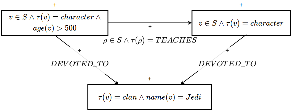
Figure 3: Example 1 GGQ.

GGQ $P_{1}$ (Figure 3) can be interpreted in natural language through the following sentence: Characters and student-teacher relationship in which both are devout of the Jedi and the teacher has more than 500 years. In this case, structural constraints are imposed through the presence of edges and through predicates that make use of $\tau$, name, and age properties. This GGQ will be verified by subgraphs where two nodes and one edge connecting them can be projected (the three elements marked as positive elements in the GGQ) verifying the imposed requirements. If there is a character who has taught himself (which would be given by a TEACHES loop) that is more than 500 years old and devout of the Jedi, any subgraph containing this node would also match this pattern. Subgraph marked as $S_{1}$ in Figure 2 matches $P_{1}$.

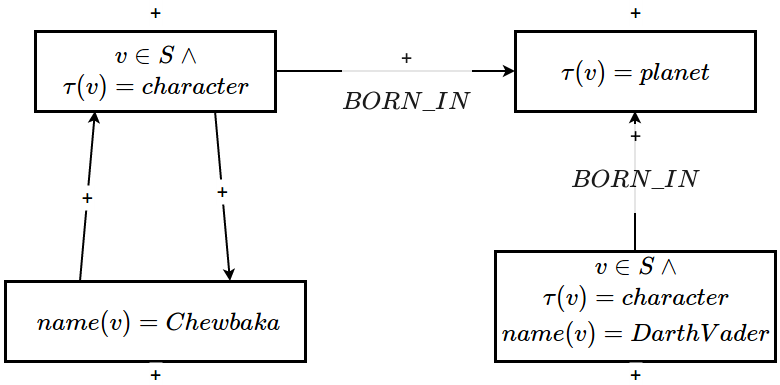
Figure 4: Example 2 GGQ.

GGQ $P_{2}$ (Figure 4) can be interpreted in natural language through the following sentence: Subgraphs containing Darth Vader and a character coming from the same planet and connected to Chewbaka. This GGQ presents a positive node representing the character Chewbaka (using $name$) and imposes a constraint requiring that one of the nodes in the evaluated subgraph has to be connected to it. Subgraph marked as $S_{2}$ in Figure 2 matches $P_{2}$.

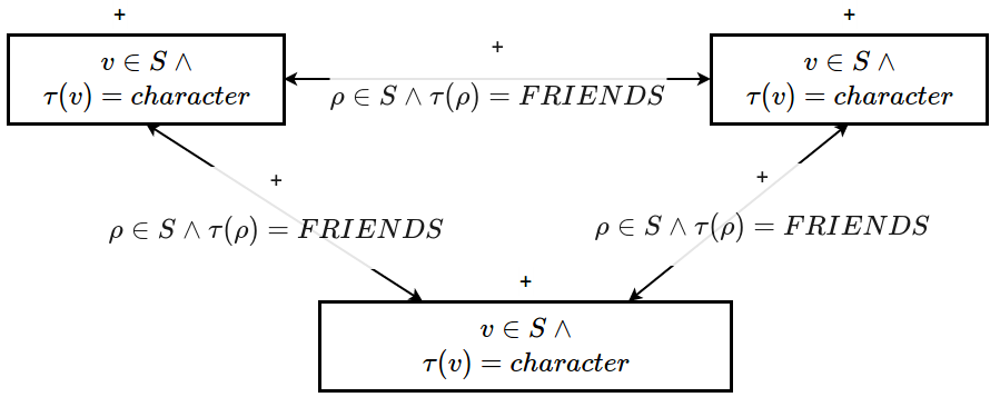
Figure 5: Example 3 GGQ.

GGQ $P_{3}$ (Figure 5) presents a cycle using FRIENDS relations, and $S_{3}$ (highlighted in Figure 2) is a subgraph that verifies it. Any subgraph containing three characters that are friends with each other will verify $P_{3}$, for example, subgraphs containing the cycle formed by Luke Skywalker, R2D2 and C3PO, or by Han Solo, Princess Leia, and Chewbaka.

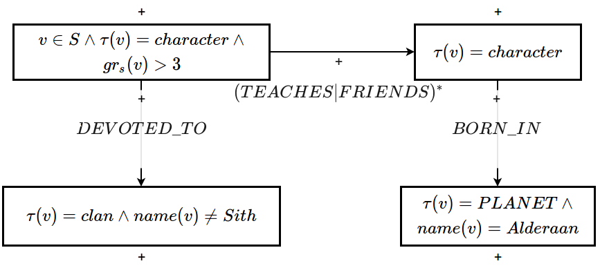
Figure 6: Example 4 GGQ.

GGQ $P_{4}$ (Figure 6) can be interpreted in natural language through the following sentence: Character with an outgoing degree greater than 3, devout of a clan other than Sith and that is connected through FRIENDS or TEACHES relationships with someone who comes from Alderaan. In this case, a regular expression has been used to express a path composed of FRIENDS or TEACHES type relationships, and an auxiliary function, $gr_{s}(v)$, has been used to refer to the outgoing degree of the $v$ node. Any subgraph containing Luke Skywalker node or Obi Wan Kenobi node will verify $P_{4}$.

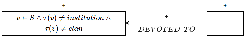
Figure 7: Example 5 GGQ.

GGQ $P_{5}$ (Figure 7) represents the query: Nodes that are not institutions or clans, but have devotees, and is only verified by nodes of type side. In this case, a node whose property $\theta$ is a tautology (represented as an empty node) has been used.

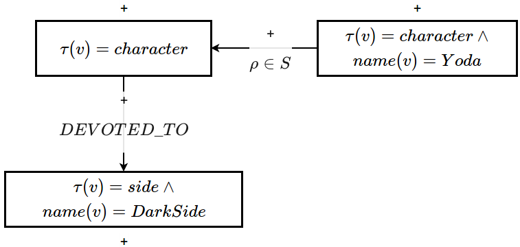
Figure 8: Example 6 GGQ.

GGQ $P_{6}$ (Figure 8) could be interpreted as: Paths connecting Yoda with characters from the Dark Side. Any subgraph containing the path (Yoda) $\rightarrow$ (Count Dooku) $\rightarrow$ (Qui Gong Jin) $\rightarrow$ (Obi Wan Kenobi) $\rightarrow$ (Darth Vader) will verify $P_{6}$.

6 Refinement Sets

In previous sections we have seen that GGQ can be interpreted as predicates over the family of subgraphs of a prefixed graph $G$. It would be interesting to obtain computationally effective ways for building complex GGQ by using basic operations to obtain families of predicates to automatically analyse the structure of subgraphs of $G$. In this section we will give a first approximation to a constructive method that is useful to perform this type of tasks.

Definition 9.

Given $Q_{1},\ Q_{2}\in GGQ$, we will say that $Q_{1}$ refines $Q_{2}$ in $G$, denoted as $Q_{1}\preceq_{G}Q_{2}$ (simply $\preceq$ when working with a prefixed graph) if:

$$\forall S\subseteq G\ (S\vDash Q_{1}\Rightarrow S\vDash Q_{2})$$

An example is shown in Figure 9. The GGQ on the left refines the GGQ on the right because in addition to requiring one of the nodes in the subgraph under evaluation to be connected to a node that does not belong to that subgraph through a publish relationship, it is also required that the target node of that relationship has an incoming edge that starts from a node that does not belong to the subgraph under evaluation.

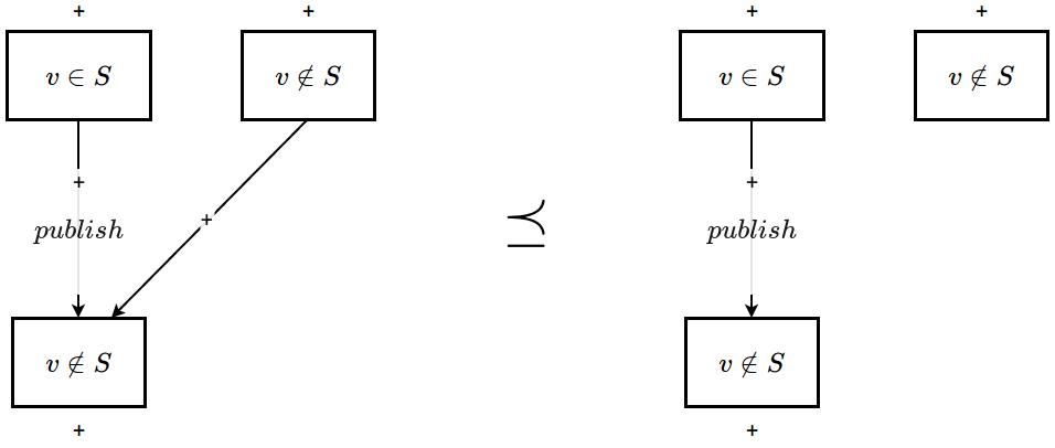
Figure 9: GGQ Refinement.

In a natural way, we can define when two GGQ are equivalent as queries, which will happen when both are verified exactly by the same subgraphs.

Definition 10.

Given $Q_{1},\ Q_{2}\in GGQ$, we will say that they are equivalents in $G$, denoted by $Q_{1}\equiv_{G}Q_{2}$ (simply $\equiv$ when working on a prefixed graph) if:

$$Q_{1}\preceq_{G}Q_{2}\ \wedge\ Q_{2}\preceq_{G}Q_{1}$$

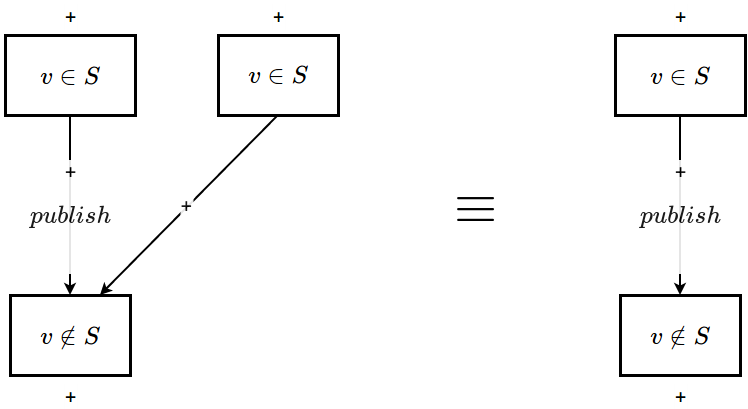
Figure 10: GGQ equivalence.

Figure 10 shows an example of equivalence. Note that the only structural difference between the two GGQ is the existence, in the left one, of a node belonging to the subgraph to be evaluated that has an output edge whose destination is a node that is not included in the subgraph under evaluation. This restriction is included in the GGQ on the right, since there is a node in the subgraph under evaluation with an edge of type publish connected to a node not belonging to that subgraph.

It is easy to prove the following result, which tells us that $\preceq_{G}$ generates a partial order relation on the GGQ considering equivalence as equality (working in the quotient space that determines equivalence).

Theorem 1.

For every property graph, $G$, $(GGQ,\preceq_{G})$ is a partial ordered set. That is:

1. $\forall Q\in GGQ\ (Q\preceq_{G}Q)$.

2. $Q_{1}\preceq_{G}Q_{2}\ \wedge\ Q_{2}\preceq_{G}Q_{1}\Rightarrow Q1\equiv_{G}Q2$.

3. $Q_{1}\preceq_{G}Q_{2}\ \wedge\ Q_{2}\preceq_{G}Q_{3}\Rightarrow Q_{1}\preceq_{G}Q_{3}$.

It is easy to verify that, in general, $\preceq_{G}$ does not generate a total order relation. To do this, just find two GGQ, $Q_{1}$ and $Q_{2}$, for which $(Q_{1}\rightarrow Q_{2})\lor(Q_{2}\rightarrow Q_{1})$ is not met. For example, if $Q_{1}$ is a GGQ composed of a single positive node with the constraint $v\in S$, and $Q_{2}$ is a GGQ also composed of a single positive node with the constraint $v\notin S$, then $Q_{1}$ will require that the subgraph under evaluation is not empty, and $Q_{2}$ will require that there be some node in the graph that does not belong to the subgraph under evaluation. Both constraints are independent so there is no implication between the predicates represented by these GGQ.

Next, we analyze the relationship between the topological structure of a GGQ and its functionality as a predicate on subgraphs. In general, it is hard trying to extract logical properties of the predicate from the structural properties of the graph representing it, but we can obtain some useful conditions that will allow us to constructively manipulate the structures to modify the interpretation of the GGQ in a controlled way.

Definition 11.

Given $Q_{1},\ Q_{2}\in GGQ$, we say that $Q_{1}$ is a $Q^{-}$-conservative extension of $Q_{2}$, and we will denote it by $Q_{2}\subseteq^{-}Q_{1}$, if:

1. $Q_{2}\subseteq Q_{1}$ (as generalized graphs, so in the $Q_{2}$ elements the values of $\alpha$ and $\theta$ should coincide for both GGQ).

2. For each negative node in $Q_{2}$, $n\in V_{Q_{2}}^{-}$, and every edge incident to it in $Q_{1}$, $e\in\gamma_{Q_{1}}(n)$, exists an edge incident to it in $Q_{2}$, $e^{\prime}\in\gamma_{Q_{2}}(n)$, imposing the same restriction, that is: $Q_{e}\equiv Q_{e^{\prime}}$.

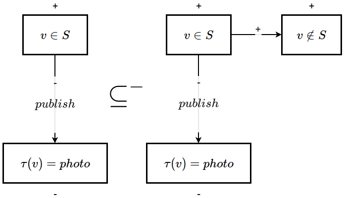
Figure 11: $Q^{-}$-conservative extension.

Figure 11 shows an example of a conservative $Q^{-}$-extension. The extension made in the GGQ on the left to get the GGQ on the right imposes new restrictions on the positive node but does not add any further restrictions to the negative node.

Since negative nodes add non-existence constraints to subgraph verification, conservative $Q^{-}$-extensions ensure that new constraints are not being added to them. Hence, we can give the next result:

Theorem 2.

Given $Q_{1},Q_{2}\in GGQ$, if $Q_{2}\subseteq^{-}Q_{1}$ then $Q_{1}\preceq Q_{2}$.

Proof.

Since $Q$-predicates associated to edges depend only on the information in the edge itself (which considers the value of $\theta$ at its incident nodes, regardless of the value of $\alpha$ in them), we can state:

$$\forall e\in E_{Q_{2}}\ ({Q_{1}}_{e}^{\alpha(e)}={Q_{2}}_{e}^{\alpha(e)})$$

Considering this fact, we analyse how the $Q$-predicates associated with the nodes for both GGQ behave:

• If $n\in V_{Q_{2}}^{-}$, since $Q_{2}\subseteq^{-}Q_{1}$, is trivial that ${Q_{1}}_{n}^{-}={Q_{2}}_{n}^{-}$.

• If $n\in V_{Q_{2}}^{+}$, then ${Q_{1}}_{n}^{+}\rightarrow{Q_{2}}_{n}^{+}$, because (we will note $\gamma_{1}$, $\gamma_{2}$ the incidence functions of $Q_{1}$ and $Q_{2}$, respectively):

  $${Q_{1}}_{n}^{+} =\exists v\in V\ \left(\bigwedge_{e\in\gamma_{1}(n)}{Q_{1}}_{e}^{\alpha(e)}\right)$$

  $$=\exists v\in V\ \left(\bigwedge_{e\in\gamma_{1}(n)\cap E_{Q_{2}}}{Q_{1}}_{e}^{\alpha(e)}\ \wedge\ \bigwedge_{e\in\gamma_{1}(n)\smallsetminus E_{Q_{2}}}{Q_{1}}_{e}^{\alpha(e)}\right)$$

  $$=\exists v\in V\ \left(\bigwedge_{e\in\gamma_{2}(n)\cap E_{Q_{2}}}{Q_{2}}_{e}^{\alpha(e)}\ \wedge\ \bigwedge_{e\in\gamma_{1}(n)\smallsetminus E_{Q_{2}}}{Q_{1}}_{e}^{\alpha(e)}\right)$$

  $$\rightarrow{Q_{2}}_{n}^{+}$$

Hence:

$$Q_{1} =\bigwedge_{n\in V_{Q_{1}}}{Q_{1}}_{n}^{\alpha(n)}=\bigwedge_{n\in V_{Q_{2}}}{Q_{1}}_{n}^{\alpha(n)}\ \wedge\ \bigwedge_{n\in V_{Q_{1}}\smallsetminus V_{Q_{2}}}{Q_{1}}_{n}^{\alpha(n)}$$

$$=\bigwedge_{n\in V_{Q_{2}}^{+}}{Q_{1}}_{n}^{\alpha(n)}\ \wedge\ \bigwedge_{n\in V_{Q_{2}}^{-}}{Q_{1}}_{n}^{\alpha(n)}\ \wedge\ \bigwedge_{n\in V_{Q_{1}}\smallsetminus V_{Q_{2}}}{Q_{1}}_{n}^{\alpha(n)}$$

$$\rightarrow\bigwedge_{n\in V_{Q_{2}}^{+}}{Q_{2}}_{n}^{\alpha(n)}\ \wedge\ \bigwedge_{n\in V_{Q_{2}}^{-}}{Q_{2}}_{n}^{\alpha(n)}\ \wedge\ \bigwedge_{n\in V_{Q_{1}}\smallsetminus V_{Q_{2}}}{Q_{1}}_{n}^{\alpha(n)}$$

$$=\bigwedge_{n\in V_{Q_{2}}}{Q_{2}}_{n}^{\alpha(n)}\ \wedge\ \bigwedge_{n\in V_{Q_{1}}\smallsetminus V_{Q_{2}}}{Q_{1}}_{n}^{\alpha(n)}$$

$$\rightarrow{Q_{2}}$$

∎

Previous result suggests that a GGQ can be refined by adding nodes (of any sign) and edges to the existing positive nodes, but because of the (negated) interpretation of $Q$-predicates associated with negative nodes, care must be taken to maintain their environment to be sure that adding more edges does not weaken the imposed conditions (and, therefore, we would not get refined predicates).

In order to obtain controlled methods of query generation, in the following we will give a constructive method to refine GGQ by unit steps. To do this, we will start by looking at how GGQ behaves when cloning nodes.

A clone consists of making copies of existing nodes, and cloning all the edges incident on them (and between them, in case we clone several nodes that are connected in the original GGQ). Of course, the cloning operation can be done on any generalized graph, not only on GGQ.

Definition 12.

Given a generalized graph $G=(V,E,\mu)$, and $W\subseteq V$, we define the clone of $G$ by duplication of $W$, denoted by $Cl_{G}^{W}$, as:

$$Cl_{G}^{W}=(V\cup W^{\prime},\ E\cup E^{\prime},\mu\cup\{(n^{\prime},\mu(n))\}_{n\in W}\cup\{(e^{\prime},\mu(e))\}_{e^{\prime}\in E^{\prime}})$$

where:

• for each $n\in W$, $n^{\prime}$ is a new node, and $W^{\prime}=\{n^{\prime}\ :\ n\in W\}$,

• $E^{\prime}$ is a set of new edges obtained from incident edges on nodes of $W$ where nodes of $W$ are replaced by copies of $W^{\prime}$ (edges connecting original nodes with cloned nodes, and edges connecting cloned nodes, are cloned).

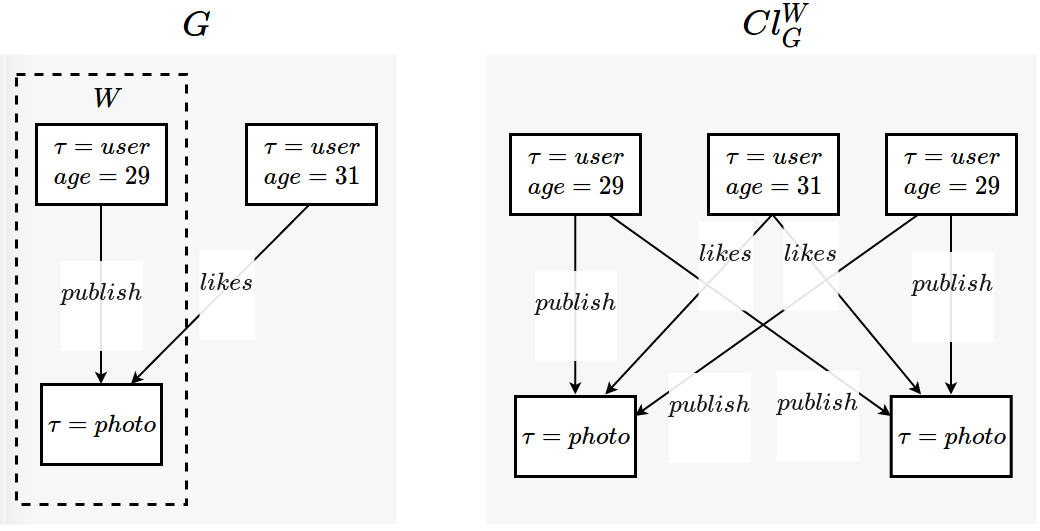
Figure 12: Clone of a graph

Figure 12 shows an example of a cloned graph by duplicating two of its nodes. In the original graph, on the left, the set of nodes to be cloned are highlighted. The result of the cloning is presented in the graph to the right.

The following result shows that cloning positive nodes does not alter the meaning of the queries.

Theorem 3.

If $Q\in GGQ$ and $W\subseteq V_{Q}^{+}$, then $Cl_{Q}^{W}\equiv Q$.

Proof.

To facilitate the notation, let $Q_{1}=Cl_{Q}^{W}$. Then, following a similar reasoning to that of the previous proof:

$$Q_{1} =\bigwedge_{n\in V_{Q_{1}}}{Q_{1}}_{n}^{\alpha(n)}$$

$$=\bigwedge_{n\in V_{Q}}{Q_{1}}_{n}^{\alpha(n)}\ \wedge\ \bigwedge_{n\in W}{Q_{1}}_{n^{\prime}}^{\alpha(n^{\prime})}$$

$$=\bigwedge_{n\in V_{Q}\smallsetminus\gamma_{Q}(W)}{Q_{1}}_{n}^{\alpha(n)}\ \wedge\ \bigwedge_{n\in\gamma_{Q}(W)}{Q_{1}}_{n}^{\alpha(n)}\ \wedge\ \bigwedge_{n\in W}{Q_{1}}_{n^{\prime}}^{\alpha(n^{\prime})}$$

$$=\bigwedge_{n\in V_{Q}\smallsetminus\gamma_{Q}(W)}Q_{n}^{\alpha(n)}\ \wedge\bigwedge_{n\in\gamma_{Q}(W)}Q_{n}^{\alpha(n)}\ \wedge\ \bigwedge_{n\in W}Q_{n}^{\alpha(n)}$$

$$=Q$$

∎

Continuing with the idea of obtaining tools to build GGQ automatically, the following concept of refinement completes the operations that we need to refine a GGQ. A refinement set forms a kind of partition of a given GGQ.

Definition 13.

Given $Q\in GGQ$, $R\subseteq GGQ$ is a refinement set of $Q$ in $G$ if:

1. $\forall\ Q^{\prime}\in R\ (Q^{\prime}\preceq_{G}Q)$

2. $\forall\ S\subseteq G\ (S\vDash Q\Rightarrow\exists!\ Q^{\prime}\in R\ (S\vDash Q^{\prime}))$

We are now ready to present some refinement sets that will allow to automate the processes of creation and modification of Generalized Graph Query. Let’s start with the simplest operation, which allows to add new nodes to an existing GGQ:

Theorem 4 (Add new node to $Q$).

Given $Q\in GGQ$ and $m\notin V_{Q}$, the set $Q+\{m\}$, formed by:

$$Q_{1} =(V_{Q}\cup\{m\},\ E_{Q},\ \alpha_{Q}\cup(m,+),\ \theta_{Q}\cup(m,T))$$

$$Q_{2} =(V_{Q}\cup\{m\},\ E_{Q},\ \alpha_{Q}\cup(m,-),\ \theta_{Q}\cup(m,T))$$

is a refinement set of $Q$ in $G$ (Fig. 13).

Proof.

We must verify that the two necessary conditions for refinement sets are verified:

1. It is trivial that $Q\subseteq^{-}Q_{1}$ and $Q\subseteq^{-}Q_{2}$, thus $Q_{1}\preceq Q$ and $Q_{2}\preceq Q$.

2. Given $S\subseteq G$ such that $S\vDash Q$. Then:

   $$Q_{1} =Q\ \wedge\ Q_{m}$$

   $$Q_{2} =Q\ \wedge\ \neg Q_{m}$$

   where $Q_{m}=\exists v\in V\ (T)$.

   If $G\neq\emptyset$, then $S\vDash Q_{1}$ and $S\nvDash Q_{2}$.

   If $G=\emptyset$, then $S\nvDash Q_{1}$ and $S\vDash Q_{2}$.

∎

Usually, $G\neq\emptyset$, hence this operation does not really refine, in the sense that $Q1\equiv Q$ and $Q2\equiv\neg T$. However, although we obtain an equivalent GGQ, this operation is very useful to add new nodes to a GGQ in order to add new restrictions to them later.

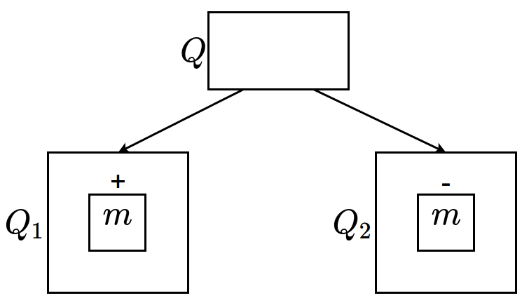
Figure 13: Refinement Add node

We proceed now to give a second refinement set that allows to create edges between existing nodes. In order to get a refinement of the original GGQ we must restrict the addition of edges to positive nodes.

Theorem 5 (Add new edge between postive nodes of $Q$).

Given $Q\in GGQ$ and $n,m\in V_{Q}^{+}$, the set $Q+\{n^{+}\overset{e^{*}}{\longrightarrow}m^{+}\}$ ($*\in\{+,-\}$), formed by (where $Q^{\prime}=Cl_{Q}^{\{n,m\}}$):

$$Q_{1} =(V_{Q^{\prime}},\ E_{Q^{\prime}}\cup\{n^{+}\overset{e^{*}}{\longrightarrow}m^{+}\},\ \theta_{Q^{\prime}}\cup(e,T))$$

$$Q_{2} =(V_{Q^{\prime}},\ E_{Q^{\prime}}\cup\{n^{+}\overset{e^{*}}{\longrightarrow}m^{-}\},\ \theta_{Q^{\prime}}\cup(e,T))$$

$$Q_{3} =(V_{Q^{\prime}},\ E_{Q^{\prime}}\cup\{n^{-}\overset{e^{*}}{\longrightarrow}m^{+}\},\ \theta_{Q^{\prime}}\cup(e,T))$$

$$Q_{4} =(V_{Q^{\prime}},\ E_{Q^{\prime}}\cup\{n^{-}\overset{e^{*}}{\longrightarrow}m^{-}\},\ \theta_{Q^{\prime}}\cup(e,T))$$

is a refinement of $Q$ in $G$ (Fig. 14).

Proof.

1. Since $Q^{\prime}$ is a clone of $Q$, and $\{n,m\}\subseteq V_{Q}^{+}$, then $Q\equiv Q^{\prime}$. In addition, $Q^{\prime}\subseteq^{-}Q_{1},Q_{2},Q_{3},Q_{4}$, thus $Q_{1},Q_{2},Q_{3},Q_{4}\preceq Q^{\prime}\equiv Q$.

2. Let us consider the predicates:

   $$P_{n} =\exists v\in V\ \left(\bigwedge_{a\in\gamma(n)}Q_{a}^{\alpha(a)}\ \wedge Q_{e^{o}}^{\alpha(e)}\right)$$

   $$P_{m} =\exists v\in V\ \left(\bigwedge_{a\in\gamma(m)}Q_{a}^{\alpha(a)}\ \wedge Q_{e^{i}}^{\alpha(e)}\right)$$

   If $S\vDash Q_{n}$ and $S\vDash Q_{m}$, then we have four mutually complementary options:

   • $S\vDash P_{n}\ \wedge\ S\vDash P_{m}\Rightarrow S\vDash Q_{1}$

   • $S\vDash P_{n}\ \wedge\ S\nvDash P_{m}\Rightarrow S\vDash Q_{2}$

   • $S\nvDash P_{n}\ \wedge\ S\vDash P_{m}\Rightarrow S\vDash Q_{3}$

   • $S\nvDash P_{n}\ \wedge\ S\nvDash P_{m}\Rightarrow S\vDash Q_{4}$

∎

If $n=m$ ($e$ is a loop) then the previous refinement set is $\{Q_{1},Q_{4}\}$.

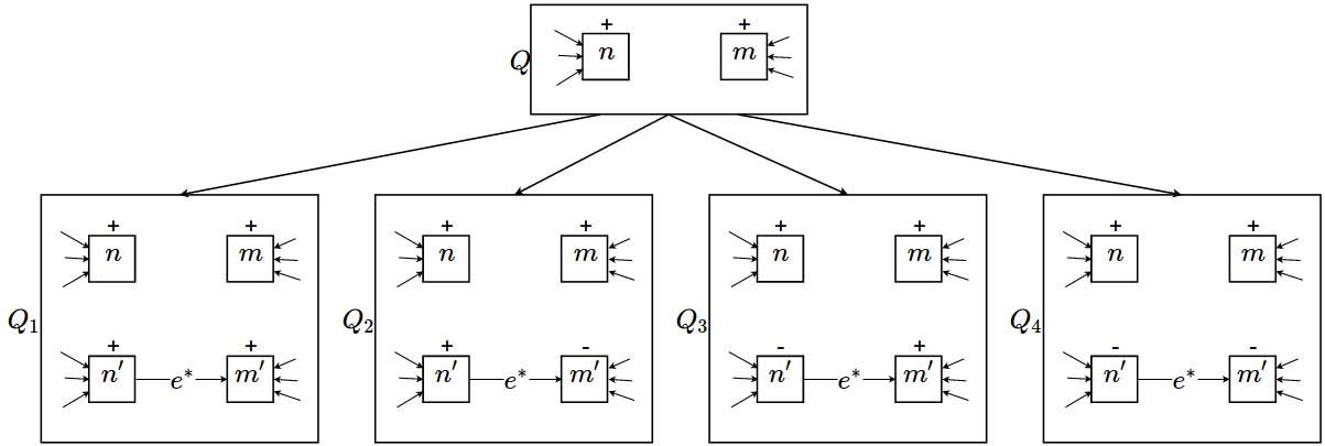
Figure 14: Refinement Add edge

Next operation adds an additional predicate to an existing edge. To keep the necessary structural conditions, this operation is restricted to positive edges connecting positive nodes.

Theorem 6 (Add predicate to positive edge between positive nodes of $Q$).

Given $Q\in GGQ$ and $n,m\in V_{Q}^{+}$, with $n^{+}\overset{e^{+}}{\longrightarrow}m^{+}$, and $\varphi\in FORM$, the set denoted by $Q+\{n^{+}\overset{e\wedge\varphi}{\longrightarrow}m^{+}\}$, formed by (where $Q^{\prime}=Cl_{Q}^{\{n,m\}}$):

$$Q1 =(V_{Q^{\prime}},\ E_{Q^{\prime}}\cup\{n^{+}\overset{e^{\prime}}{\longrightarrow}m^{+}\},\ \theta_{Q^{\prime}}\cup(e^{\prime},\theta_{e}\wedge\varphi))$$

$$Q2 =(V_{Q^{\prime}},\ E_{Q^{\prime}}\cup\{n^{+}\overset{e^{\prime}}{\longrightarrow}m^{-}\},\ \theta_{Q^{\prime}}\cup(e^{\prime},\theta_{e}\wedge\varphi))$$

$$Q3 =(V_{Q^{\prime}},\ E_{Q^{\prime}}\cup\{n^{-}\overset{e^{\prime}}{\longrightarrow}m^{+}\},\ \theta_{Q^{\prime}}\cup(e^{\prime},\theta_{e}\wedge\varphi))$$

$$Q4 =(V_{Q^{\prime}},\ E_{Q^{\prime}}\cup\{n^{-}\overset{e^{\prime}}{\longrightarrow}m^{-}\},\ \theta_{Q^{\prime}}\cup(e^{\prime},\theta_{e}\wedge\varphi))$$

is a refinement set of $Q$ in $G$ (Fig. 15).

Proof.

The proof is similar to those shown in previous results. ∎

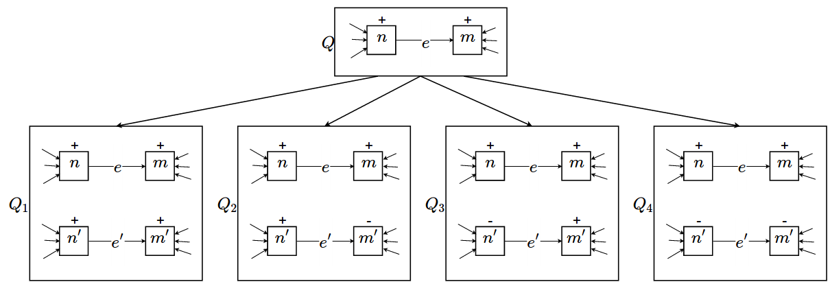
Figure 15: Refinement Add predicate to edge

Finally, the last operation adds predicates to existing nodes. Again, we restrict this operation to cases when the affected nodes are positive (the node where the predicate is added, and those connected to it).

Theorem 7 (Add predicate to positive node with positive environment in $Q$).

Given $Q\in GGQ$, $n\in V_{Q}^{+}$, with $\mathcal{N}_{Q}(n)\subseteq V_{Q}^{+}$, and $\varphi\in FORM$. We define the set $Q+\{n\wedge\varphi\}$ formed by:

$$\{Q_{\sigma}=(V_{Q^{\prime}},E_{Q^{\prime}},\alpha_{Q^{\prime}}\cup\sigma,\theta_{Q^{\prime}}\cup(n^{\prime},\theta_{n}\wedge\varphi))\ :\ \sigma\in\{+,-\}^{\mathcal{N}_{Q}(n)}\}$$

where $Q^{\prime}=Cl_{Q}^{\mathcal{N}_{Q}(n)}$, and $\{+,-\}^{\mathcal{N}_{Q}(n)}$ is the set of all possible assignations of signs to elements in $\mathcal{N}_{Q}(n)$.

Then $Q+\{n\wedge\varphi\}$ is a refinement set of $Q$ in $G$ (Fig. 16).

Proof.

The proof is similar to the previous cases. It is only necessary to take into account that, when modifying the node $n$, not only the $Q$-predicate associated with it is modified but also those from all its adjacent nodes, and the set of functions $\{+,-\}^{\mathcal{N}_{Q}(n)}$ cover all possible sign assignment for the nodes in the environment. ∎

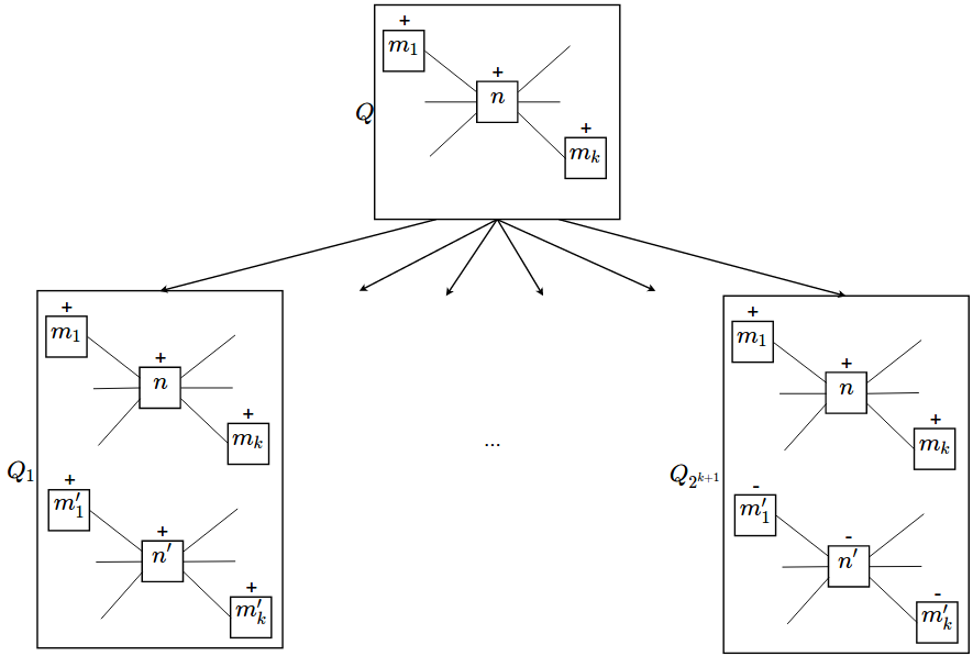
Figure 16: Refinement Add predicate to node

It should be noted that these refinements generate structures that can be simplified. Next we provide some operations to simplify a GGQ and to obtain another equivalent and simpler one.

Definition 14.

Given $Q\in GGQ$, $Q^{\prime}\subseteq Q$ is redundant in $Q$ if $Q\equiv Q-Q^{\prime}$. Where $Q-Q^{\prime}$ is the subgraph of $Q$ given by:

$$(V_{Q}\smallsetminus V_{Q^{\prime}},E_{Q}\smallsetminus(E_{Q^{\prime}}\cup\{\gamma(n):\ n\in V_{Q^{\prime}}\}),\mu_{Q})$$

Let us see a first result that allows to obtain simplified versions of a GGQ by removing positive redundant nodes:

Theorem 8.

Given $Q\in GGQ$, and $n\in V_{Q}^{+}$ such that exists $m\in V_{Q}$ verifying:

• $\alpha(n)=\alpha(m)$, $\theta_{n}\equiv\theta_{m}$.

• For each $e\in\gamma(n)$, exists $e^{\prime}\in\gamma(m)$, verifying $\alpha(e)=\alpha(e^{\prime})$, $\theta_{e}=\theta_{e^{\prime}}$ and $\gamma(e)\smallsetminus\{n\}=\gamma(e^{\prime})\smallsetminus\{m\}$.

Then, $n$ is redundant in $Q$.

Essentially, $m$ is a clone of $n$, but possibly with more edges connected. We can obtain a similar result for edges:

Theorem 9.

Given $Q\in GGQ$, and two edges, $e,e^{\prime}\in E_{Q}$, such that $n^{+}\overset{e}{\longrightarrow}m^{+}$ and $n^{+}\overset{e^{\prime}}{\longrightarrow}m^{+}$. If $\theta_{e}\rightarrow\theta_{e^{\prime}}$ then $e^{\prime}$ is redundant in $Q$.

From these two results we can give simplified versions of the previous refinement sets, grouping positive nodes and positive edges when, after initial cloning, the sign of the duplicate element has been maintained with the original, as well as in the cases where the sign has been maintained and an additional predicate has been added. Figures 17 to 19 shows representations of the refinement sets $Q+\{n\wedge\varphi\}$, $Q+\{n^{+}\overset{e\wedge\varphi}{\longrightarrow}m^{+}\}$ and $Q+\{n\wedge\varphi\}$ applying these simplifications.

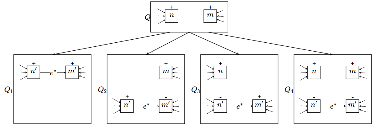
Figure 17: Refinement Add edge (simplified)

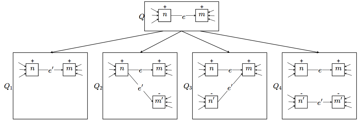
Figure 18: Refinement Add predicate to edge (simplified)

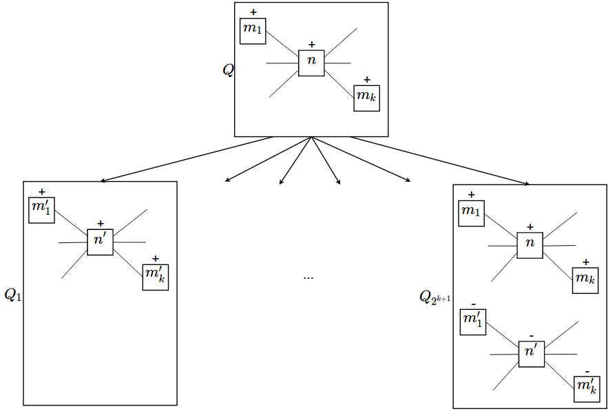
Figure 19: Refinement Add predicate to node (simplified)

For example, the following sequence of refinements constructs the pattern $P_{5}$ (Fig. 20):

$$Q_{1} =Q_{\emptyset}+\{n_{1}\}$$

$$Q_{2} =Q_{1}+\{n_{1}\land(v\in S\land\tau(v)\neq\mathtt{institution}\land\tau(v)\neq\mathtt{clan}\}$$

$$Q_{3} =Q_{2}+\{n_{2}\}$$

$$Q_{4} =Q_{3}+\{n_{2}\overset{e_{1}}{\longrightarrow}n_{1}\}$$

$$P_{5} =Q_{4}+\{n_{2}\overset{e_{1}\land(\tau(\rho)=\mathtt{DEVOTED\_TO})}{\longrightarrow}n_{1}\}$$

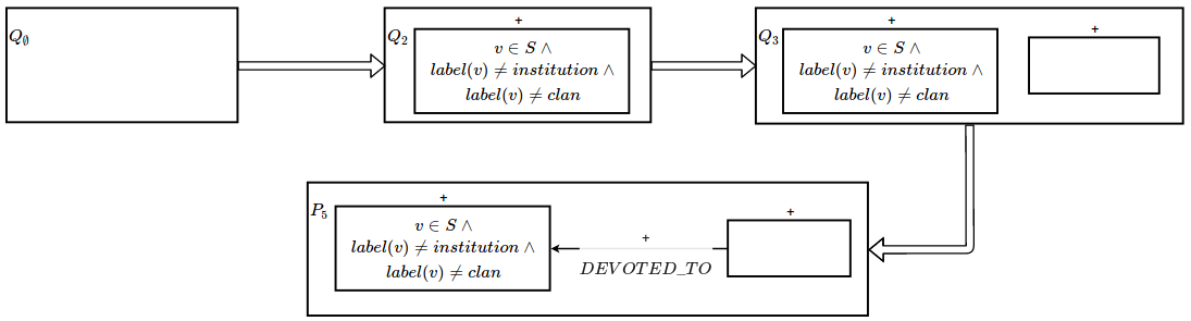
Figure 20: Sequences of refinements for $P_{5}$

From the structure of a GGQ it is not easy to obtain a complementary GGQ with it. However, there are many analysis on property graphs (or generalized graphs) where we need to work with sequences of queries verifying some properties of containment and complementarity as predicates. The refinements presented in this section come to cover this gap and to allow, for example, the construction of an embedded partition tree with the nodes labelled as follows (Fig. 21):

• The root node is labelled with $Q_{0}$ (some initial GGQ).

• If a tree node is labelled with $Q$, and $R=(Q_{1},\dots,Q_{n})$ is a refinement set of $Q$, then its child nodes are labelled with the elements of $R$.

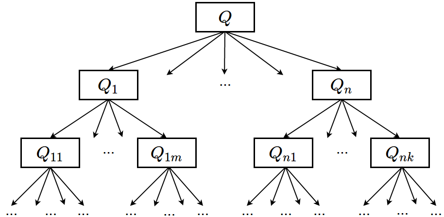
Figure 21: Refinements tree

Note that the construction of this tree completely depends on the refinement chosen in each branch, and the initial GGQ.

The refinements presented here are only one option, but not the only one. For example, we could consider refinements that, instead of adding constraints to positive elements, lighten the conditions over negative elements, and using disjunction of predicates instead of conjunction of them.

7 Conclusions and Future Work

In this work we have presented a framework to evaluate subgraphs immersed in property graphs (more generally, in generalized graphs) that can be used in discovery procedures over relational data. We want this framework to verify several requirements:

• To use the same grammar for the queries and for the structures to evaluate. Thanks to the expressive power of generalized graphs we have presented a query tool that can be expressed by using generalized graphs.

• To provide well-founded basis that would assure the queries behave consistently and robustly. These results have been obtained by studying the relationships between the topological structure of the query and the logical meaning of the query.

• In addition, we have provided a controlled way to construct GGQ by means of atomic operators that translates the topological control of the construction into a logical control of the meaning. In this sense, we have introduced a first family of refinements to achieve this goal.

Because relational data can be viewed as graphs, and queries can be viewed as pattern searchs, most query languages in databases can be viewed as (perhaps primitive) graph pattern matching tools. In this paper we have analysed some of the existing query tools as well as the feasibility to be used in automatic procedures. One of these tools, Selection Graphs, allows to evaluate records in relational databases through acyclic patterns that can be refined by using basic operations, and allowing to obtain complementary patterns in each case. They do not require an exact projection of the pattern representing the selection graph onto the subgraph to be evaluated, but rather the fulfillment of a series of predicates expressed in the pattern. We must remember that if a projection is required when carrying out the verification of a pattern, the task of evaluating the non-existence of certain elements becomes hard. Specifically, selection graphs evaluate the existence / non-existence of paths incidents into the record under evaluation (they are only capable of evaluating individual records) by verifying a conjunction of predicates associated to those paths, and it can be seen as the evaluation of existence of a tree rooted in the node that represents the record under evaluation.

Generalized Graph Query extends the concept of selection graphs allowing the evaluation of general subgraphs, beyond a single node, the use of more powerful predicates and allowing cyclical patterns. As it becomes a requirement not to use a projection for the verification of a pattern, these objectives have been achieved by extending the form of evaluation, which can be seen as the evaluation of a tree rooted in every node from the pattern (allowing the edges to be identified with paths in the graph). Consequently, it manages more complex structures. The intersections between the various trees and the constraints imposed on the nodes allow the evaluation of cyclical patterns in the GGQ, something that had not been achieved in previous proposals.

As we have mentioned, like selection graphs, GGQ can be modified and constructed from refinements, but unlike the simple case of selection graphs, refinements of GGQ are usually not binary, resulting in sets of size $2^{k}$ (where $k$ is the number of modified predicates). In general, refinements result in embedded partitions of the structures they evaluate, making them ideal tools for white-box machines learning procedures. After carrying out a first (but fully functional) proof-of-concept implementation, it has been experimentally demonstrated the practical usefulness of GGQ framework.

An explicit use of these capabilities has already been carried out in knowledge discovery procedures, specifically in the GGQ-ID3 algorithm, which makes use of Generalized Graph Query as tests in the nodes of decision trees. The relationship between GGQ and GGQ-ID3 is equivalent to that between selection graphs and the algorithm MRDTL [12]. In the experiments carried out in this context it is shown that GGQ-ID3 is able to extract interesting GGQ patterns that can be used in complex tasks.

On the other hand, more complex refinement families can be created (for example, combining the refinement add edge with adding property to an edge in a single step) to thereby reduce the number of steps to get complex GGQ and to get more powerful atomic steps. If this option is carried out properly (unifying the refinements according to the frequency of occurrence of structures in a graph, for example) faster version of algorithms making use of GGQ can be obtained. In this case the improvement in efficiency is achieved by sacrificing the possibility of covering a wider query space. A minimal and robust set of refinement operations have been offered in this work, but they are not intended to be optimal for every learning task. Consequently, GGQ represents a powerful and simple query tool of controlled complexity, suitable for automatic construction and to be used in white-box multi-relational machine learning algorithms.

In the future work that derives from the development presented here, it is worth mentioning that, since GGQ are constructed using the generalized graph structure (that allows the definition of hypergraphs in a natural way), with slightly modifications GGQ can evaluate hypergraphs with properties. Hence, the extension of Generalized Graph Query to Generlized Hypergraph Query is a natural step that is worth considering. The development of different refinement sets in correspondence to the learning task or the type of graph to query is a future line of research. In addition, the automatic generation of such sets from statistics extracted from the graph to be analysed can lead to important optimizations in GGQ automatic construction processes. Finally, it should be noted that GGQ is already being used by discovery / learning procedures, such as the multi-relational tree-building algorithm GGQ-ID3 named above, and thanks to its good properties, it is a great candidate to be used by other algorithms of this type.

References

- [1] Cypher into patterns. http://neo4j.com/docs/stable/cypher-intro-patterns.html.
- [2] Cypher introduction. http://neo4j.com/docs/stable/cypher-introduction.html.
- [3] Faisal Alkhateeb, Jean-Francois Baget, and Jérôme Euzenat. RDF with regular expressions. PhD thesis, INRIA, 2007.
- [4] Pablo Barceló, Leonid Libkin, and Juan L. Reutter. Querying graph patterns. In Proceedings of the Thirtieth ACM SIGMOD-SIGACT-SIGART Symposium on Principles of Database Systems, PODS ’11, pages 199–210, New York, NY, USA, 2011. ACM.
- [5] Mariano P. Consens and Alberto O. Mendelzon. Graphlog: A visual formalism for real life recursion. In Proceedings of the Ninth ACM SIGACT-SIGMOD-SIGART Symposium on Principles of Database Systems, PODS ’90, pages 404–416, New York, NY, USA, 1990. ACM.
- [6] Wenfei Fan. Graph pattern matching revised for social network analysis. In Proceedings of the 15th International Conference on Database Theory, ICDT ’12, pages 8–21, New York, NY, USA, 2012. ACM.
- [7] Wenfei Fan, Jianzhong Li, Shuai Ma, Nan Tang, and Yinghui Wu. Adding regular expressions to graph reachability and pattern queries. In Serge Abiteboul, Klemens Böhm, Christoph Koch, and Kian-Lee Tan, editors, ICDE, pages 39–50. IEEE Computer Society, 2011.
- [8] Wenfei Fan, Jianzhong Li, Shuai Ma, Nan Tang, Yinghui Wu, and Yunpeng Wu. Graph pattern matching: From intractable to polynomial time. Proc. VLDB Endow., 3(1-2):264–275, September 2010.
- [9] Brian Gallagher. Matching structure and semantics: A survey on graph-based pattern matching. AAAI FS, 6:45–53, 2006.
- [10] S. Gupta. Neo4j Essentials. Community experience distilled. Packt Publishing, 2015.
- [11] Arno J. Knobbe, Arno Siebes, Danil Van Der Wallen, and Syllogic B. V. Multi-relational decision tree induction. In In Proceedings of PKDD’ 99, Prague, Czech Republic, Septembre, pages 378–383. Springer, 1999.
- [12] Héctor Ariel Leiva, Shashi Gadia, and Drena Dobbs. Mrdtl: A multi-relational decision tree learning algorithm. In Proceedings of the 13th International Conference on Inductive Logic Programming (ILP 2003, pages 38–56. Springer-Verlag, 2002.
- [13] R. Milner. Communication and Concurrency. Prentice-Hall, Inc., Upper Saddle River, NJ, USA, 1989.
- [14] Neelamadhab Padhy and Rasmita Panigrahi. Multi relational data mining approaches: A data mining technique. CoRR, abs/1211.3871, 2012.
- [15] Juan L. Reutter. Graph Patterns: Structure, Query Answering and Applications in Schema Mappings and Formal Language Theory. PhD thesis, The school where the thesis was written, Laboratory for Foundations of Computer Science School of Informatics University of Edinburgh, 2013.
- [16] Toby Segaran, Colin Evans, Jamie Taylor, Segaran Toby, Evans Colin, and Taylor Jamie. Programming the Semantic Web. O’Reilly Media, Inc., 1st edition, 2009.
- [17] Oskar van Rest, Sungpack Hong, Jinha Kim, Xuming Meng, and Hassan Chafi. Pgql: a property graph query language. In Proceedings of the Fourth International Workshop on Graph Data Management Experiences and Systems, page 7. ACM, 2016.
- [18] Lei Zou, Lei Chen, and M. Tamer Özsu. Distance-join: Pattern match query in a large graph database. Proc. VLDB Endow., 2(1):886–897, August 2009.