Robust information divergences for model-form uncertainty arising from sparse data in random PDE

Abstract.

We develop a novel application of hybrid information divergences to analyze uncertainty in steady-state subsurface flow problems. These hybrid information divergences are non-intrusive, goal-oriented uncertainty quantification tools that enable robust, data-informed predictions in support of critical decision tasks such as regulatory assessment and risk management. We study the propagation of model-form or epistemic uncertainty with numerical experiments that demonstrate uncertainty quantification bounds for (i) parametric sensitivity analysis and (ii) model misspecification due to sparse data. Further, we make connections between the hybrid information divergences and certain concentration inequalities that can be leveraged for efficient computing and account for any available data through suitable statistical quantities.

Key words. uncertainty quantification, epistemic, sparse data, data-informed, information divergence, concentration inequalities, sensitivity analysis, model misspecification, random PDE, steady-state flow

AMS subject classifications. 65C50, 60H35, 94A17

1. Introduction

1.1. Context and objectives

Stochastic modeling of complex systems involves a multilayered process where various sources of uncertainty are accounted for at different stages. In a goal-oriented framework, the ultimate focus of the model is to estimate a quantity of interest (QoI) that depends on model outputs in order to make predictions in support of risk management, regulatory assessment, performance optimization, safety or reliability engineering, and other critical decision tasks ([46, 11]). Since model outputs can be sensitive to distributional assumptions made throughout this process, the analysis of uncertainty in a QoI is essential. Additionally, applications in physically relevant settings often pose challenges not present in the conceptual formulation that demand incorporating data into the modeling process. The modeling of complex systems in physically relevant settings, therefore, requires goal-oriented uncertainty quantification (UQ) tools that allow one to distinguish sources of uncertainty present in the system with a view toward making robust, data-informed predictions.

Figure 1. The modeling of steady-state subsurface flow in physically relevant settings demands goal-oriented UQ tools that allow one to distinguish different sources of uncertainty present in the system with a view toward making robust, data-informed predictions in support of decision tasks (adapted from [46]). A key challenge concerning the propagation of epistemic uncertainty from inputs to outputs is examined in detail in Figure 2.

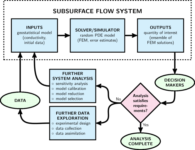
In the present work, we consider the modeling of steady-state subsurface flow, a complex system depicted in Figure 1 that has important applications in hydrology, carbon sequestration, and petroleum engineering ([2, 25, 1, 16]). The core mathematical problem involves a random partial differential equation (PDE) of elliptic type that describes the physics of steady-state flow. The stochastic coefficient in the PDE represents a conductivity field given by a geostatistical model with properties inferred from relevant data. Robust predictions for a QoI, and in particular techniques for quantifying the propagation uncertainty from the geostatistical model, are critical to inform decision tasks. However, in physically relevant settings the complexity of subsurface porosity and the sparsity of available data pose a number of challenges.

We seek to address some of these challenges using techniques from applied probability. Information divergences, the primary tool that we will employ, have been successfully applied to problems in stochastic dynamics ([11, 21, 34, 31]). Based on the Donsker–Varadhan variational principle ([20]), information divergences provide goal-oriented UQ bounds that first appeared in [11] and have since undergone various extensions and further analysis ([42, 4, 38]). However, the application of information divergences to complex real-world systems, for example, systems containing multiple scales, multiple levels of fidelity, and multiple sources and types of uncertainty, have only been shallowly explored. The multifaceted nature of the modeling task for our problem of interest requires a formulation that distinguishes multiples sources of uncertainty to which we attach varying levels of confidence while also considering computational challenges to practical implementation. Further, we wish to incorporate data into this process in a systematic manner that complements existing inference procedures and we provide new perspectives on the hybrid information divergences that enable data-informed predictions.

For our system of interest, we develop a novel application of hybrid information divergences to study the propagation of model-form uncertainty related to the inputs of the goal-oriented framework in Figure 1. Model-form or epistemic uncertainty ([35, 36, 52, 26, 37, 48, 49]) in this context expresses ignorance in the nature of the geostatistical model due to the sparsity of available data arising for example from lacking priors, incomplete information, and missing science. This uncertainty represents a modeling error that we evaluate as the weak error between a QoI obtained from a nominal and an alternative geostatistical model for the inputs. These hybrid information divergences build on traditional UQ by enabling bounds across model predictions that would otherwise be computationally expensive using standard techniques, e.g. Monte Carlo (MC) or generalized polynomial chaos (gPC) expansions.

Importantly, the hybrid nature of the information divergences employed here allows us to represent, aggregate, and distinguish various sources of uncertainty by treating distinct sources under performance measures that allow us to attach varying levels of confidence to different parts of the model. These hybrid divergences have the form of a relative entropy penalized by a risk-sensitive hybrid performance measure, similar in flavor to the Gibbs variational formula in statistical mechanics ([23]), that strikes a balance between data-dependent quantities (relative entropy) and physics-dependent quantities (risk-sensitive performance measures i.e. cumulant generating functions that depend on the output of the forward model). On the one hand, these bounds are robust in that for a fixed nominal model they bound all alternative models within a given information budget. On the other hand, these bounds are tight in that there exists an alternative model within a given information budget for which the bounds are attained as equality ([4, 32]). We mention that this information budget, when viewed as an allowable level of model-form uncertainty, is philosophically similar to the privacy level introduced in the context of Rényi divergence in a model for differential privacy ([19]). Numerical experiments are included here to demonstrate the application of this theory for (i) a straightforward UQ task in section 3 concerning parametric sensitivity analysis and (ii) a more exploratory UQ task in section 4 featuring bounds for model misspecification due to sparse data that are not captured by small parametric perturbations.

Although a mathematically rigorous hybrid modeling framework was first introduced in [11], with variations in [41], here we explore the application of hybrid goal-oriented divergences to stochastic models of complex systems involving random PDE and also provide new insights on uncertainty arising from data while providing a new perspective on the information divergences as data-informed UQ bounds. In particular, we apply hybrid information divergences to complex systems where the forward modeling involves random PDEs where the random field is inferred from real-world data and gPC cannot be used due to log-normality ([24]). We explore how the hybrid information divergences quantify model-form uncertainty while also providing a perspective linking model-form uncertainty to sparse data. This brings new insights on the use of information divergence for predictive modeling with data by studying how changes to data result in alternative models that are not small perturbations of the nominal model. Further, we explore connections with certain well-known concentration inequalities ([17]) that can be leveraged for efficient computing; this latter approach was recently introduced and applied to model problems in [32] and we extend these ideas here to models for complex systems involving random PDE where the stochastic fields are infinite dimensional and inferred from real-world data. The concentration inequalities yield non-intrusive upper and lower uncertainty quantification bounds that involve statistical quantities more easily computed than the cumulant generating functions in earlier works on information divergences.

The hybrid divergences presented here provide a UQ framework that is well suited to the particular application of interest for a number of reasons. Firstly, hybrid information divergences provide a natural way of representing and distinguishing various sources of uncertainty arising in the distinct layers of the modeling process for complex systems that complement existing inference procedures while allowing us to attach varying levels of confidence in different components of our model. Secondly, the structure of the hybrid divergences allows UQ computations to be carried out non-intrusively by interfacing with existing simulation and sampling methods for the random PDE such as the popular MC finite element method (FEM). Thirdly, the hybrid information divergences encapsulate “worst case” scenarios within a rigorous formulation similar to a robust optimization perspective ([6]) making them appropriate deliverables in the context of decision support. In the remainder of this section, we formulate the model problem and some of the main UQ challenges that motivate our approach.

1.2. Formulation of the model problem

Presently we detail the main layers comprising the subsurface flow system in Figure 1 each in turn.

1.2.1. Random PDE model

For a given probability space $(\Omega,\mathcal{F},P)$, we consider the random PDE in the unknown $u$,

(1) $$-\nabla\cdot(a(\omega,x)\nabla u(\omega,x))=f(x),\quad\text{for }x\in\Gamma\subset\textbf{R}^{d},$$

subject to $u=u_{0}$ on $\partial\Gamma$, with given data $u_{0}$, source term $f:\Gamma\to\textbf{R}$, and stochastic conductivity $a:\Omega\times\Gamma\to\textbf{R}$. Arising from Darcy’s law with continuity, 1 is a model for steady-state flow or diffusion. In subsurface hydrology, problem 1 models time-independent groundwater flow where $u$ might represent a water head (pressure) or the concentration of a containment ([2, 16]). The existence of a unique pathwise variational solution $u$ to 1 follows by assuming sufficiently regular data and boundedness of the conductivity ([9]). For simplicity of presentation we consider the steady-state system 1, however, the theory that follows can be applied to other forward models for subsurface flow and/or transport such as (reaction-)advection-dispersion equations [55, 2].

In the sequel we consider the standard, continuous piecewise-linear FEM approximation $\bar{u}(\omega)\approx u(\omega)$ of the pathwise variational solution of 1 and then sample QoIs via a MC method. This approach is favored for the application of interest since the finite element solution $z=(\bar{u}_{n})$ is a possibly high dimensional random vector due to the low-regularity of the conductivity field. A discrete projection of the conductivity field $y=(\bar{a}_{n})\approx a(\omega)$ is then used when forming the stiffness matrix in the FEM solver. Other approaches, such as the stochastic Galerkin ([44]) or stochastic collocation ([5]) methods are typically advantageous when the conductivity possesses more regularity; being non-intrusive, our approach is also applicable using these methods. Regarding the analysis of FEM errors, a priori estimates are available in [10] and computable goal-oriented estimates for problems with rough stochastic conductivities are in [33].

1.2.2. QoIs

The goal of problem 1 is to estimate a QoI,

$$\operatorname{\mathbf{E}}_{P}[g(u)]=\int_{\Omega}g(u(\omega,x))\mathrm{d}P,$$

for a given goal functional $g$ in support of a decision task. The numerical experiments in this work focus on goal functionals that yield statistics of point estimates, $g(u)=u(x)$, and indicator goal functionals, $g(u)=\textbf{1}_{A}$ that correspond to failure probabilities,

(2) $$\operatorname{\mathbf{E}}_{P}[\textbf{1}_{A}]=P(A)\,,$$

for events $A\subset\Omega$ such as $A:=\{\omega:u(\omega,x_{0})>k\}$, the event that the solution at $x_{0}\in\Gamma$ exceeds a threshold $k$. In this instance, QoIs might involve solving the steady-state system 1 for contaminant concentrations and hydraulic heads or fluxes (e.g. heads $u(x)$, fluxes $q(x):=-a(x)\nabla u(x)$) to predict QoIs or forecast future conditions ([2]). QoIs such as failure probabilities, for example, the probability of a contaminant exceeding a threshold or a contaminant plume reaching a specified zone, would then factor into larger probabilistic risk assessment, i.e. concerning contamination of groundwater, that would represent perhaps one system fault or route to failure ([55]). A QoI that is meant to provide a quantitative description of the system can be highly sensitive to distributional assumptions on the underlying geostatistical model. This poses a key challenge for the support of decision tasks and highlights the importance of understanding the propagation of modeling error due to the geostatistical model in order to quantify uncertainty in a QoI.

1.2.3. Geostatistical model

Subsurface materials are observed to be heterogeneous over each of the problem scales related to experimental measurements ([15]). In applications to physically relevant settings, fully resolving a model for $a$ requires more data than is possible to acquire. Uncertainty in the problem data is subsequently captured through a geostatistical model for $a$ that typically takes the form of a log-normal random field that possesses low regularity. Such a field is characterized by its mean, $\mu(x)=\operatorname{\mathbf{E}}[\log a(x)]$, and covariance,

$$C(x,\tilde{x})=\operatorname{Cov}[\log a(x),\log a(\tilde{x})],\qquad\text{for }x,\tilde{x}\in\Gamma.$$

These quantities describe the spatial structure in terms of statistics between different locations and are nontrivial to model for heterogeneous media. In applications, these quantities are typically further assumed to have a parametric form where the hyperparameters that describe $\mu$ and $C$ are representative of physical properties that can theoretically be measured using relevant data. Inference procedures for the hyperparameters range from classical geostatistical methods, that rely on fitting variograms using likelihoods or moments, to more advanced Bayesian methodologies ([27]). For applications in physically relevant settings, the complex physics of subsurface porosity results in sparse data that diminishes our confidence in the form of the geostatistical model. In the next section, we further motivate and formulate these challenges.

1.3. UQ challenges

The rough log-normal random fields that are typically used to capture the heterogeneity of subsurface materials produce computational challenges at the level of the solver and when analyzing model outputs (Figure 1). For example, gPC methods exhibit slow convergence due to the log-normality ([24]). As noted in [13], the correlation lengths involved in the geostatistical model are typically short with respect to the problem domain, hence stochastic Galerkin methods yield high dimensional QoIs, but still too large to guarantee a separation of scales, an obstacle to stochastic homogenization techniques. In addition, the complex physics also affects the acquisition and reliability of data.

The data used to identify the salient features of the geostatistical model are typically sparse due to costs arising from a number of confounding factors. In this context, data may come from either empirical or experimental measurements collected by domain scientists at different scales of the problem. Then, relevant data, for instance, the permeability field, needs to be assimilated and inferred from these measurements. For example, a geostatistical model for the conductivity might be based on empirical porosity and water retention measurements from a controlled laboratory experiment in combination with variogram fitting methods ([22]) or on hydraulic head measurements from in situ field tests in combination with a Bayesian inverse problem ([45]). In both cases, the geostatistical model is determined from data whose availability is limited and whose reliability should be questioned. The combination of these factors influences our confidence in the form of the geostatistical model.

Therefore, we view the geostatistical model as a source of model-form or epistemic uncertainty. Although theoretically reducible, eliminating epistemic uncertainty entirely for subsurface flow is not feasible due to the prohibitive cost of collecting sufficient data. Additionally, the physical system has other sources of randomness such as aleatoric uncertainty, or variability, in the model inputs, solver, and outputs and may have independent sources of epistemic uncertainty that arise in each of these layers. All of this randomness propagates to the QoI and influences the decision task. A less refined approach, in contrast to the one considered here, is to assume that epistemic uncertainty can be modeled by aleatoric uncertainty which is typically the case in a standard MC approximation when one assumes that a distribution for each uncertain aspect of the system exists ([46, 11]).

The main UQ challenges postulated above are summarized as follows:

• represent and distinguish various sources of uncertainty in the system;

• propagate model-form uncertainty;

• inform decision tasks through robust data-informed deliverables;

• quantify the impact of sparse data on predictions in a goal-oriented framework; and

• analyze heterogeneity of subsurface physics.

The final challenge point, related to the solver layer of Figure 1, leads to considerations that impact the random PDE model, such as UQ for multi-phase flows, and are beyond the scope of the present work. The focus of the present work is instead toward addressing the first four challenge points, that have important implications for the inputs, outputs, further analysis, and data layers of the model in Figure 1. In particular, we address the propagation of model-form uncertainty by employing hybrid representations of information divergences, introduced in the next section, that allow us to represent and distinguish various sources of randomness.

2. Hybrid information divergences and model-form uncertainty

2.1. Propagation of model-form uncertainty

A key challenge addressed in this work concerns the propagation of model-form uncertainty within the goal-oriented framework in Figure 1. We view the propagation of model-form uncertainty as a modeling error or model bias,

(3) $$\mathcal{E}(Q,P;g(\bar{u})):=\operatorname{\mathbf{E}}_{Q}[g(\bar{u})]-\operatorname{\mathbf{E}}_{P}[g(\bar{u})],$$

the weak error between a QoI evaluated under a nominal measure $P$ and an alternative measure $Q$. We do not give a method for choosing the nominal model $P$ or the alternative model $Q$, but only a method for reasoning quantitatively about the effect that different modeling choices will have on decision support. In this context we view the nominal model $P$ as a computationally tractable model or surrogate presently being used to inform decision tasks; in subsurface flow, the nominal model would be derived from the conceptual model chosen by a geoscientist that summarizes what is known about the hydrogeological system ([2, 55]). Respectively, the alternative model $Q$ can either be viewed as a fine scale model that is not computationally tractable (for instance $P$ as a coarse-grained model for $Q$) or, in view of sparse data, as another surrogate that is also plausible ($Q$ equally as plausible as the nominal model $P$). In either case, the weak error 3 suggests how different modeling choices impact model predictions of the QoI. We seek representations for $P$ and $Q$ that will allow us to track the propagation of uncertainty from model inputs to outputs as illustrated in Figure 2. We observe that although the propagation of model-form uncertainty is controlled by 3, quantifying the propagation directly using 3 will be computationally infeasible (cf. Corollary 1 below).

Figure 2. Detail of the dashed box in Figure 1 that demonstrates model-form uncertainty in the geostatistical model propagating through the random PDE solver, with distribution 5, to a QoI. The propagation is controlled by the weak error 3 between a QoI evaluated under a nominal and alternative model with distributions 4.

As the conductivity field $a$ is a source of epistemic uncertainty, the distribution of $y=(\bar{a}_{n})$ is not known and it will be of natural interest to study the propagation of this source of uncertainty in particular and to compare the effects of different solver inputs as suggested in Figure 2. To this end, we consider

(4) $$\text{nominal }y\sim\gamma\quad\text{or}\quad\text{alternative }y\sim\lambda,$$

for measures $\gamma$ and $\lambda$ on a Polish space $\mathcal{Y}$, arising from the geostatistical models proposed for $a$. For example, the nominal and alternative distribution of $y$ could be associated with small parametric perturbations or to completely different models within a parametric family. The discrete solution $z=(\bar{u}_{n})$, resulting from a given algorithm for solving the random PDE, represents a source of variability as it is modeled by a stochastic process. Theoretically, $z$ has a known distribution given by $\nu$, on a Polish space $\mathcal{Z}$, that depends on the solver and $\bar{a}$. In general, even if the distribution of $a$ is prescribed it may not be tractable to sample from $\nu$ directly. Instead, the conditional distribution of $\bar{u}$ given $y$, that is,

(5) $$z=(\bar{u}_{n})\sim\nu(\mathrm{d}z\mid y),$$

is a computable quantity that we will evaluate using a FEM solver as indicated in Figure 2. Theoretically, qualitatively different distributions for $y$ (i.e. geostatistical models with more or less regularity) could necessitate different solvers; in this case, one could also include $\nu^{\prime}$ different from $\nu$. For simplicity here we assume that the same solver with distribution $\nu(\mathrm{d}z\mid y)$ is used with respect to the nominal and alternative model. Stating our objective more formally, we consider 3 between a QoI sampled with respect to the full Bayesian network for the nominal measure $P=\gamma\otimes\nu$ and alternative measure $Q=\lambda\otimes\nu$. The preceding analysis suggests that bounds for model outputs that distinguish these different sources of uncertainty can be obtained by concentrating on a special case of the hybrid bounds proposed in [11] that rely on the conditional distribution 5.

2.2. Representing and distinguishing sources of uncertainty

To achieve the desired bounds, we represent $g(\bar{u})$ in terms of a variational form

$$g(\bar{u})=h(y,z)$$

that distinguishes between the epistemic variable $y$, related to $\bar{a}$, and aleatoric variable $z$, related to $\bar{u}$. That is, for $Q=\lambda\otimes\nu$ we define a hybrid performance measure $h$ by

(6) $$\operatorname{\mathbf{E}}_{\lambda\otimes\nu}[h]=\int_{\mathcal{Y}}\int_{\mathcal{Z}}h(y,z)\nu(\mathrm{d}z\mid y)\lambda(\mathrm{d}y)=\int_{\Omega}g(\bar{u})\mathrm{d}Q=\operatorname{\mathbf{E}}_{Q}[g(\bar{u})].$$

For simplicity in the presentation we assume that $z=(\bar{u}_{n})$ is only a source of variability and that the $u_{0}$ and $f$ in 1 are deterministic; however, observe that the representation 6 can easily be extended to characterize various uncertain aspects of the system by introducing multiple integrals that aggregate and distinguish each independent source of randomness.

A key observation is that the hybrid performance measure 6 can then be expressed as

(7) $$\operatorname{\mathbf{E}}_{\lambda\otimes\nu}[h]=\operatorname{\mathbf{E}}_{\lambda}[H^{g}]\,,$$

where the random variable $H^{g}(y)$ is the marginal performance measure given by,

(8) $$H^{g}(y)=\int_{\mathcal{Z}}h(y,z)\nu(\mathrm{d}z\mid y)\,,$$

for $y\in\mathcal{Y}$. $H^{g}$ encodes the propagation of the model-form uncertainty to the ensemble solution of the random PDE (the outputs in Figure 2). Approximation of a QoI depending on the goal functional $g$ amounts to a standard MC estimate for the sample mean of $H^{g}$ where $H^{g}$ is computed in a non-intrusive manner using any available algorithm for the solver. Next, we introduce an important information theoretic tool that will allow us to measure differences between models suggested for epistemic variables.

2.3. Relative entropy in UQ

The relative entropy, or Kullback–Leibler divergence, quantifies the discrepancy between two distributions (see for example [50, §A.5]). Given probability measures $\gamma$ and $\lambda$, such that $\lambda\ll\gamma$, the relative entropy of $\lambda$ with respect to $\gamma$ is

$$\operatorname{\mathcal{R}}(\lambda\mid\gamma)=\int\log\frac{\mathrm{d}\lambda(y)}{\mathrm{d}\gamma(y)}\lambda(\mathrm{d}y),$$

and we note that $\operatorname{\mathcal{R}}(\lambda\mid\gamma)\geq 0$ with equality if and only if $\lambda=\gamma$ almost everywhere (the Gibbs inequality). For distributions that belong to a general exponential family, closed formulas exist for the relative entropy ([28, 43]). For example, the relative entropy for $d$-dimensional multivariate Gaussian distributions $\lambda=\mathcal{N}(\mu_{i},\Sigma_{i})$ and $\gamma=\mathcal{N}(\mu_{j},\Sigma_{j})$ is given by

(9) $$\operatorname{\mathcal{R}}(\lambda\mid\gamma)=\frac{1}{2}\left(\log|\Sigma_{j}|-\log|\Sigma_{i}|+\operatorname{tr}\left(\Sigma_{j}^{-1}\Sigma_{i}\right)+(\mu_{i}-\mu_{j})^{\top}\Sigma_{j}^{-1}(\mu_{i}-\mu_{j})-d\right),$$

where $|\cdot|$ denotes the determinant.

The relative entropy is related to the observable $H^{g}$ via the Legendre transform of the cumulant generating functional $\log\operatorname{\mathbf{E}}_{\gamma}[e^{H^{g}}]$. We will use this well known fact from Large Deviations Theory to study the propagation of model-form uncertainty in Figure 2. This representation balances data- and physics-based components and in particular we use this new perspective in section 4 to provide data-informed UQ bounds. The proof of the following lemma is well known and available in [20], nevertheless we provide it for the convenience of the reader.

Lemma 1.

Let the marginal performance measure $H^{g}$ 8 be measurable and bounded and let $\gamma$ be a probability measure on $(\Omega,\mathcal{F})$. Then

$$\log\operatorname{\mathbf{E}}_{\gamma}[e^{H^{g}}]=\sup_{\lambda\ll\gamma}\left\{\operatorname{\mathbf{E}}_{\lambda}[H^{g}]-\operatorname{\mathcal{R}}(\lambda\mid\gamma)\right\}.$$

Proof.

Define $\nu$ as $\mathrm{d}\nu/\mathrm{d}\gamma=e^{H^{g}}/\operatorname{\mathbf{E}}_{\gamma}[e^{H^{g}}]$. Then

$$-\operatorname{\mathcal{R}}(\lambda\mid\gamma)+\operatorname{\mathbf{E}}_{\lambda}[H^{g}] =-\operatorname{\mathbf{E}}_{\lambda}\!\!\left[\log\frac{\mathrm{d}\lambda}{\mathrm{d}\gamma}\right]+\operatorname{\mathbf{E}}_{\lambda}[H^{g}]$$

$$=-\operatorname{\mathbf{E}}_{\lambda}\!\!\left[\log\frac{\mathrm{d}\lambda}{\mathrm{d}\nu}\right]-\operatorname{\mathbf{E}}_{\lambda}\!\!\left[\log\frac{\mathrm{d}\nu}{\mathrm{d}\gamma}\right]+\operatorname{\mathbf{E}}_{\lambda}[H^{g}]$$

$$=-\operatorname{\mathcal{R}}(\lambda\mid\nu)+\log\operatorname{\mathbf{E}}_{\gamma}[e^{H^{g}}].$$

This proves the lemma and $\nu$ is necessarily the suprimizing measure. ∎

Lemma 1 is the key ingredient in the proof of Theorem 1, concerning hybrid information divergences, that follows in the next section.

2.4. Goal-oriented hybrid divergences for modeling error

We begin by defining a hybrid risk-sensitive performance measure,

(10) $$\Lambda_{\gamma}(c,H^{g}):=\frac{1}{c}\log\int_{\mathcal{Y}}e^{c\left(\int_{\mathcal{Z}}h(y,z)\nu(\mathrm{d}z\mid y)-\operatorname{\mathbf{E}}_{\gamma}[H^{g}]\right)}\gamma(\mathrm{d}y)=\frac{1}{c}\log\operatorname{\mathbf{E}}_{\gamma}[e^{c(H^{g}-\operatorname{\mathbf{E}}_{\gamma}[H^{g}])}],$$

for a parameter $c>0$ that depends on the goal function $g$ through the marginal performance measure $H^{g}$. As suggested by the last equality in 10, $\Lambda_{\gamma}$ is a weighted cumulant generating functional (log moment generating functional) for the centered random variable $c(H^{g}-\operatorname{\mathbf{E}}_{\gamma}[H^{g}])$. The idea behind Theorem 1 below is to apply Lemma 1 to 10 to obtain a family of bounds indexed by $c$. The best bound is then found by minimizing over $c$,

(11) $$\Xi(\lambda\mid\gamma;H^{g}):=\inf_{c>0}\left\{\Lambda_{\gamma}(c,H^{g})+\frac{1}{c}\operatorname{\mathcal{R}}(\lambda\mid\gamma)\right\}\,,$$

which defines a goal-oriented hybrid information divergence. This insight was first made in [21] where information divergences were applied to stochastic dynamical systems with single sources of uncertainty; we contrast the naive implementation of the information divergences from [21] with the hybrid information divergences developed here for our problem of interest after the proof of Theorem 1. That 11 is a divergence, i.e. $\Xi(\lambda\mid\gamma;H^{g})\geq 0$ and $\Xi(\lambda\mid\gamma;H^{g})=0$ if and only if $\lambda=\gamma$ almost everywhere or $H^{g}$ is constant $\gamma$-a.s., follows analogously to the proof of Theorem 2.7 in [21]. A bound for the weak error 3 specialized to 11 is formulated as follows.

Theorem 1 (Hybrid Information Divergence).

For a probability measure $\gamma$, measurable marginal performance measure $H^{g}$, and finite $\Lambda_{\gamma}(c,H^{g})$ in a neighborhood about $c=0$, the bound

(12) $$-\Xi(\lambda\mid\gamma;-H^{g})\leq\operatorname{\mathbf{E}}_{Q}[g(\bar{u})]-\operatorname{\mathbf{E}}_{P}[g(\bar{u})]\leq\Xi(\lambda\mid\gamma;H^{g})$$

holds for any probability measure $\lambda$ such that $\operatorname{\mathcal{R}}(\lambda\mid\gamma)<\infty$ where $Q=\lambda\otimes\nu$ and $P=\gamma\otimes\nu$. Further, the goal-oriented divergence can be linearized with respect to the relative entropy,

(13) $$\Xi(\lambda\mid\gamma;\pm H^{g})=\sqrt{\operatorname{Var}_{\gamma}\left[H^{g}\right]}\sqrt{2\operatorname{\mathcal{R}}(\lambda\mid\gamma)}+O(\operatorname{\mathcal{R}}(\lambda\mid\gamma))\,.$$

Proof.

For any bounded and measurable observable $H^{g}$, replacing $H^{g}$ in Lemma 1 with $c(H^{g}-\operatorname{\mathbf{E}}_{\gamma}[H^{g}])$, for $c>0$, yields

$$\log\operatorname{\mathbf{E}}_{\gamma}[e^{c(H^{g}-\operatorname{\mathbf{E}}_{\gamma}[H^{g}])}]=\sup_{\lambda\ll\gamma}\left\{c(\operatorname{\mathbf{E}}_{\lambda}[H^{g}]-\operatorname{\mathbf{E}}_{\gamma}[H^{g}])-\operatorname{\mathcal{R}}(\lambda\mid\gamma)\right\}.$$

This variational characterization yields the bounds

(14a) $$\operatorname{\mathbf{E}}_{\lambda}[H^{g}]-\operatorname{\mathbf{E}}_{\gamma}[H^{g}]\leq\frac{1}{c}\log\operatorname{\mathbf{E}}_{\gamma}[e^{c(H^{g}-\operatorname{\mathbf{E}}_{\gamma}[H^{g}])}]+\frac{1}{c}\operatorname{\mathcal{R}}(\lambda\mid\gamma)\quad\text{and}$$

(14b) $$\operatorname{\mathbf{E}}_{\lambda}[H^{g}]-\operatorname{\mathbf{E}}_{\gamma}[H^{g}]\geq-\frac{1}{c}\log\operatorname{\mathbf{E}}_{\gamma}[e^{c(H^{g}-\operatorname{\mathbf{E}}_{\gamma}[H^{g}])}]-\frac{1}{c}\operatorname{\mathcal{R}}(\lambda\mid\gamma)$$

where the optimal bound can be found by minimizing 14a (respectively maximizing 14b) over $c>0$. This implies 12 for any measurable and bounded $H^{g}$. This bound can be extended to any measurable $H^{g}$, by considering 14a and 14b with $H^{g}_{a,b}-\operatorname{\mathbf{E}}_{\gamma}[H^{g}]$ in place of $H^{g}-\operatorname{\mathbf{E}}_{\gamma}[H^{g}]$ in the cumulant generating functional, where $H^{g}_{a,b}=[H^{g}\vee(-a)]\wedge b$ for $a,b\in\textbf{R}$, and then letting $a\to\infty$ under the monotone convergence theorem and $b\to\infty$ using the dominating function $e^{c(H^{g}-\operatorname{\mathbf{E}}_{\gamma}[H^{g}])}$, following the argument given in [21, p. 86]. The linearization 13 arises from an asymptotic expansion at $\operatorname{\mathcal{R}}(\lambda\mid\gamma)=0$, i.e. when $\lambda$ is a perturbation of $\gamma$, which relies on first proving that the optimization problems in 12 admit a unique solution $c^{*}(\rho)$. The details follow analogously from the proofs of Lemma 2.11 and Theorem 2.12 in [21]. ∎

Theorem 1, suggests an upper and lower bound for the weak error 3 between model predictions with respect to the full Bayesian network formulation for the nominal model $P$ and alternative model $Q$. 12 trades the problem of sampling the weak error 3, that involves sampling the QoI with respect to both $Q$ and $P$, for an optimization problem 11 that only requires sampling a cumulant generating functional with respect to $P$. This enables comparisons among models in contrast to the optimal uncertainty bounds in [47]. In the present work, we do not compare model outputs to experimentally observed flow variables nor do we assimilate data from experimental observations to re-calibrate the probabilistic models in the experiments. Due to the sparsity of available data, model verification is not typically employed in geostatistical modeling as all available data is used to formulate and calibrate the model ([18]).

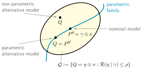
We reiterate that bounds 12 are non-intrusively computable and tight. The structure of the marginal performance measure $H^{g}$ allows the cumulant generating functional appearing in 12 to be sampled non-intrusively (i.e. without changing the code for simulating the forward model) with respect to the nominal model $\gamma$ (the proposed computationally tractable model). Recall that $H^{g}$ 8 is intimately related to the propagation of epistemic uncertainty in Figure 2 from the inputs to the solver/simulator. In contrast to classical bounds derived from the Pinsker or Chapman–Robbins inequalities ([14, 57]), 12 is tight in that equality is attainable for a given QoI by a suitable $\lambda$ within a given relative entropy distance of the nominal model, as suggested in Figure 3 (for a full discussion on tightness see [32]).

In general, the hybrid information divergence 11 allows one to express different levels of confidence in various components in a complex system and we refer to these bounds as hybrid divergences following the terminology in [11]. For complex subsurface flow systems (Figure 1), 11 possess a form aligned with our goal of evaluating model-form uncertainty as a modeling error. In contrast, the goal-oriented information divergences from [21] defined on product measures has the form

(15) $$\Xi(\lambda\otimes\nu\mid\gamma\otimes\nu;h):=\inf_{c>0}\left\{\Lambda_{\gamma\otimes\nu}(c,h)+\frac{1}{c}\operatorname{\mathcal{R}}(\lambda\otimes\nu\mid\gamma\otimes\nu)\right\}\,,$$

where $\Lambda_{\gamma\otimes\nu}$ is the standard risk-sensitive performance measure given by

(16) $$\Lambda_{\gamma\otimes\nu}(c,h)=\frac{1}{c}\log\operatorname{\mathbf{E}}_{\gamma\otimes\nu}[e^{c(h-\operatorname{\mathbf{E}}_{\gamma\otimes\nu}[h])}]\,.$$

The divergence 15 incorporates the epistemic and aleatoric variables in a balanced manner that does not conform with the asymmetrical way that we view these different sources of uncertainty. Moreover, in the present setting it may not be possible to sample $h$ directly whereas the marginal performance measure $H^{g}$ is the natural quantity to sample in the context of the MC FEM approach. To make the connection between the original divergence and hybrid divergence concrete, we observe that 15 depends on the representation for $h$ while 11 depends on $H^{g}$ (cf. 7). While both 15 and 11 yield valid bounds for the weak error 3, we have that

$$\Xi(\lambda\mid\gamma;H^{g})\leq\Xi(\lambda\otimes\nu\mid\gamma\otimes\nu;h)=\Xi(Q\mid P;g)$$

due to Jensen’s inequality applied to the exponential of 8. That is, the naive implementation of 15 contains (not surprisingly) more uncertainty than the hybrid divergence 11.

In the sequel, we write

$$\Xi_{+}:=\Xi\,,\quad\text{and}\quad\Xi_{-}(\cdot\mid\cdot;H^{g}):=-\Xi(\cdot\mid\cdot;-H^{g})$$

to have a short notation for distinguishing the upper bound from the lower bound. Next, we emphasizes that 12 applies to all alternative models within a given information budget.

Corollary 1.

Let the assumptions of Theorem 1 hold and let $\rho:=\operatorname{\mathcal{R}}(\lambda\mid\gamma)$. Then

(17) $$-\inf_{c>0}\left\{\Lambda_{\gamma}(c,-H^{g})+\frac{\rho}{c}\right\}\leq\operatorname{\mathbf{E}}_{Q}[g(\bar{u})]-\operatorname{\mathbf{E}}_{P}[g(\bar{u})]\leq\inf_{c>0}\left\{\Lambda_{\gamma}(c,H^{g})+\frac{\rho}{c}\right\}$$

for all $Q=\eta\otimes\nu$ such that $\operatorname{\mathcal{R}}(\eta\mid\gamma)\leq\rho$.

Corollary 1 suggests a bound across an infinite dimensional family of alternative models,

$$\mathcal{Q}:=\{Q=\eta\otimes\nu:\operatorname{\mathcal{R}}(\eta\mid\gamma)\leq\rho\}\,,$$

that includes both parametric and non-parametric perturbations as depicted in Figure 3. We observe that the bound 17 requires sampling the cumulant with respect to the nominal model and then optimizing over $c$ once for a given $\rho$ and QoI. In contrast, computing the weak error 3 directly for every $Q\in\mathcal{Q}$ would be computationally infeasible. Although we cannot give a general insight on how to interpret the information budget, one can get a sense of the family of alternative models that fall within a given budget, for example, how qualitatively different a model you can buy for a fixed amount of relative entropy, by computing a relative entropy landscape (cf. Figures 5c and 6b). In the context of Rényi divergence in a model of differential privacy, [19] introduces a level of privacy, $\alpha$, that is philosophically similar to $\rho$ when viewed as an allowable level of model-form uncertainty.

Figure 3. For a given information budget $\rho$, Corollary 1 suggests tight and computable upper and lower bounds for the weak error 3 between a nominal model $P$ for every alternative model $Q\in\mathcal{Q}$, an infinite dimensional family that includes both parametric and non-parametric perturbations. The information budget $\rho$ can be interpreted as an allowable level of model-form uncertainty.

Remark 1:

For any invertible transformation $T$,

$$\operatorname{\mathcal{R}}(\lambda\mid\gamma)=\operatorname{\mathcal{R}}(T(\lambda)\mid T(\gamma)),$$

from the Data Processing Inequality (see for example [28]). Thus, we can replace the distribution of the conductivity $\bar{a}$ with the distribution of $\log\bar{a}$ in any relative entropy statement without a loss of information.

2.5. Uncertainty intervals

We end this section with another perspective on 12 for data-informed prediction. For a given nominal model $P=\gamma\otimes\nu$, 12 can be rewritten as

$$\operatorname{\mathbf{E}}_{P}[g(\bar{u})]-\Xi(\lambda\mid\gamma;-H^{g})\leq\operatorname{\mathbf{E}}_{Q}[g(\bar{u})]\leq\operatorname{\mathbf{E}}_{P}[g(\bar{u})]+\Xi(\lambda\mid\gamma;H^{g}),$$

yielding an uncertainty interval for an alternative model prediction. The alternative model $Q=\lambda\otimes\nu$ falls within a region of confidence given by the nominal model prediction $\pm\Xi$, i.e. $\operatorname{\mathbf{E}}_{Q}[g(\bar{u})]\in\operatorname{\mathbf{E}}_{P}[g(\bar{u})]\pm\Xi(\lambda\mid\gamma;\pm H^{g})$, providing a guarantee on a QoI with respect to an alternative model $Q$. For failure probabilities 2 (such as the goal functionals $g_{1}$ and $g_{2}$ to appear in sections 3 and 4), the hybrid information divergences have a particularly simple form that gives a confidence interval for the $Q$-probability of failure.

Theorem 2 (Uncertainty Interval for $Q$-failure).

For a nominal model $P=\gamma\otimes\nu$, let $g(\bar{u})=\textbf{1}_{A}$ for $A\subset\Omega$ with $P(A)=p$ and let $\rho:=\operatorname{\mathcal{R}}(\lambda\mid\gamma)$. Then,

$$-\min_{c>0}\left\{\frac{1}{c}\log(pe^{-c}+1-p)+\frac{\rho}{c}\right\}\leq Q(A)\leq\min_{c>0}\left\{\frac{1}{c}\log(pe^{c}+1-p)+\frac{\rho}{c}\right\},$$

for every alternative model $Q=\eta\otimes\nu$ such that $\operatorname{\mathcal{R}}(\eta\mid\gamma)\leq\rho$.

Proof.

The risk-sensitive performance measure is

(18) $$\Lambda_{\gamma}(c,\pm H^{g})=\frac{1}{c}\log\operatorname{\mathbf{E}}_{\gamma}[e^{\pm c(H^{g}-\operatorname{\mathbf{E}}_{\gamma}[H^{g}])}]=\frac{1}{c}\log(pe^{\pm c}+1-p)\mp p$$

and thus the bounds follows immediately from 12. ∎

The remainder of this paper focuses on applications of the hybrid information divergences to UQ. First, in section 3 we apply Theorem 1 to derive bounds for parametric sensitivity analysis by considering alternative models that can be represented by small parametric perturbations of the nominal model. Then in section 4 we examine a more exploratory UQ task and derive bounds for model misspecification due to sparse data where the nominal and alternative models cannot, in general, be described by small perturbations. Finally, in section 5, we leverage the connection between certain concentration inequalities and the hybrid divergences for efficient computing.

3. The simplest UQ application: parametric sensitivity analysis

Presently we apply the tools developed in section 2 to sensitivity analysis when the model inputs are specified by a parametric geostatistical model. This setting represents the simplest UQ application of the hybrid information divergences in that we have tight control over the perturbations and hence over the alternative models under consideration (see Figure 3 where the parametric perturbations are tightly controlled). Although simple, the example nonetheless represents an important UQ task and allows us to demonstrate the tightness and robustness of the bounds derived from the hybrid information divergences. In principle, this approach can be applied to study non-parametric models, i.e. models that are infinite dimensional in the parameter space, such as a gPC representation of the conductivity in combination with a stochastic Galerkin method for the solver. However, we note that for our specific application of interest with a lognormal conductivity such an approximation is not guaranteed to converge due to Proposition 4.2 in [24].

In the section that follows, we begin by providing notation and motivation for the parametric sensitivity analysis. In section 3.2 we give Corollary 2 containing a cheaply computed bound that can be used to efficiently screen for insensitive parameter directions. Then in section 3.3, we apply Theorem 1 to obtain accurate and robust bounds for sensitivity analysis. Finally, in section 3.4 we provide details on the implementation. We emphasize that although a one-dimensional example problem is considered, the techniques demonstrated easily scale to higher dimensions.

3.1. Parametric geostatistical models and sensitivity indices

For a given probability space $(\Omega,\mathcal{F},P)$ we consider the two-point boundary value problem

(19) $$-(a^{\theta}(\omega,x)u^{\prime}(\omega,x))^{\prime}=1,\qquad\text{for }x\in[0,1],$$

subject to $u(\omega,0)=0$ and $a^{\theta}(\omega,1)u^{\prime}(\omega,1)=1$, where randomness enters only through a scalar-valued log-normal process $a^{\theta}$ that depends on a vector of hyperparameters $\theta\in\mathbf{R}^{k}$. In particular, we consider $\log a^{\theta}$ with mean $\mu$ and squared-exponential type two-point covariance function $C$ given by,

(20) $$C(r)=\begin{cases}\sigma^{2}e^{-|r/\sqrt{2}\ell|^{2}},&\text{for }r>0,\\ \tau^{2}+\sigma^{2},&\text{for }r=0,\end{cases}$$

where $r=|x-\tilde{x}|$ for $x,\tilde{x}\in[0,1]$.

For the mean and covariance above, $a^{\theta}$ is a stationary, isotropic random field where the hyperparameters of interest are $\theta=(\mu,\sigma^{2},\ell,\tau^{2})\in\mathbf{R}^{4}$. In applications, these hyperparameters have geostatistical interpretations that play a role in fitting the model for $a^{\theta}$ from data; $\mu$ is related to the overall trend, $\sigma^{2}$ is related to the sill measurement, $\ell$ is related to the spatial correlation length, and $\tau^{2}$ is related to the nugget effect or microscale variability ([27]). The sample paths of the process $a^{\theta}$ exhibit qualitatively different behavior across a range of hyperparameter values and it is therefore natural to question the sensitivity of a QoI with respect to parametric modeling assumptions on the conductivity field. With a view toward employing the hybrid information divergences in section 2, we denote the finite dimensional distributions $(\bar{a}^{\theta}_{n})\sim\gamma$ and $(\bar{a}^{\theta^{\prime}}_{n})\sim\gamma^{\prime}$ where $\theta^{\prime}=\theta+\epsilon v$ is a small perturbation for $\epsilon>0$ in the direction $v\in\mathbf{R}^{4}$ with $|v|=1$. Then we consider the joint probability measures $P^{\theta}=\gamma\otimes\nu$ and $P^{\theta^{\prime}}=\gamma^{\prime}\otimes\nu$ that correspond to the nominal and perturbed parameters of the geostatistical model where we denote the distribution of the corresponding finite element solution by $(\bar{u}_{n})\sim\nu(\mathrm{d}z\mid\cdot)$. We would like to understand the sensitivity of $\operatorname{\mathbf{E}}_{P^{\theta}}[g(\bar{u})]$ with respect to distributional assumptions on $P^{\theta}$ and in particular to quantify worst-case scenarios concerning this sensitivity with a view toward informing decision tasks.

For a given goal functional $g$, we define the sensitivity index,

(21) $$\mathcal{S}(v,\theta;g)=\theta\lim_{\epsilon\to 0}\frac{\operatorname{\mathbf{E}}_{P^{\theta+\epsilon v}}[g(\bar{u})]-\operatorname{\mathbf{E}}_{P^{\theta}}[g(\bar{u})]}{\epsilon},$$

that describes the sensitivity of a given goal functional $g$ with respect to $\theta$ in the direction $v$, provided $\mathcal{S}$ depends continuously on $\theta$. In the limit of small $\epsilon$, $\mathcal{S}$ converges to the logarithmic derivative $\partial_{\log\theta}\operatorname{\mathbf{E}}_{P^{\theta}}[g(\bar{u})]=\theta\partial_{\theta}\operatorname{\mathbf{E}}_{P^{\theta}}[g(\bar{u})]$, a scaling chosen to control for differences in the orders of magnitude of the hyperparameters.

Computing a classical gradient approximation of $\mathcal{S}$ in each parameter direction for each QoI represents a nontrivial computational cost even for the simple model problem 19. A naive finite difference approximation of the sensitivity index would require sampling with respect to both $P^{\theta}$ and $P^{\theta^{\prime}}$ where each sample involves a call to a PDE solver for each direction $v$ in $\theta^{\prime}=\theta+\epsilon v$. Moreover, such a gradient approximation introduces a bias error that must be taken into account; for a better approximation of the sensitivity, corresponding to small $\epsilon$, the variance of the approximation increases and therefore our confidence of it decreases. While reduced variance methods for gradient approximations exist ([29, 30]), our direction here is an altogether different one. In contrast, 12 in Theorem 1 yields tight non-gradient based estimates for the sensitivity 21 that only require sampling with respect to the nominal model $P^{\theta}$. Before considering these more accurate bounds in section 3.3, we first demonstrate in section 3.2 a cheaply computed bound, derived from expansion 13 in Theorem 1, that can be used to screen for insensitive parameter directions.

3.2. Fast screening for small perturbations

While it is always advantageous if the number of parameters to include in the full sensitivity analysis can be reduced, the efficiency gain is acute when simulations are computationally expensive such as involving successive calls to a PDE solver. Following from 13 in Theorem 1, we consider a linearization specialized to small perturbations that relies on the Fisher Information matrix (FIM). As the FIM and can be computed cheaply, that is, without sampling, the linearized bound can be used to efficiently screen for insensitive parameter directions. We recall that the FIM for a parametric family of distributions $P^{\theta}$ is given by

$$\mathcal{I}(\theta):=\int_{\textbf{R}^{d}}\nabla_{\theta}\log p(x;\theta)(\nabla_{\theta}\log p(x;\theta))^{\top}p(x;\theta)\mathrm{d}x,$$

where $p(x;\theta)$ is the density conditional on the value of $\theta$ (a classical definition from [58]).

Corollary 2 (Efficient Screening).

For a smooth parametric family $P^{\theta}$ and $\epsilon>0$,

$$\frac{1}{\epsilon}|\operatorname{\mathbf{E}}_{P^{\theta^{\prime}}}[g(\bar{u})]-\operatorname{\mathbf{E}}_{P^{\theta}}[g(\bar{u})]|\leq\sqrt{\operatorname{Var}_{\gamma}[H^{g}]}\sqrt{v^{\top}\mathcal{I}(\theta)v}+O(\epsilon)$$

where $\mathcal{I}(\theta)$ is the FIM associated with $P^{\theta}$. Hence

(22) $$|\mathcal{S}(v,\theta;g)|\leq\theta\sqrt{\operatorname{Var}_{\gamma}[H^{g}]}\sqrt{v^{\top}\mathcal{I}(\theta)v}.$$

The bounds suggested in Corollary 2 are for small $\epsilon$ perturbations of the nominal model in terms of the variance of the marginal performance measure $H^{g}$ and the FIM. Recall that $H^{g}$ is related to the distribution of the QoI given the distribution of input parameters. Reminiscent of the variance-bias trade-off of other information information-based criterion for assessing model selection in statistics (for example Akaike Information Criterion and Bayesian Information Criterion [8]), importantly 22 is a goal-oriented quantity that incorporates the output of the forward model $H^{g}$.

Corollary 2 follows from the general non-infinitesimal linearization 13 by noticing that the relative entropy has the expansion

$$\operatorname{\mathcal{R}}(P^{\theta+\epsilon v}\mid P^{\theta})=\frac{\epsilon^{2}}{2}v^{\top}\mathcal{I}(\theta)v+O(\epsilon^{3})$$

when considering small perturbations to a smooth parametric family of probability measures; the complete proof follows from results in [21]. A similar linearization has been used in chemical kinetics to screen for insensitive parameter directions in the situation where the number of parameters is large ([3, 56]). For both a multivariate normal distribution and log-normal distribution characterized by mean $\mu(\theta)$ and covariance $\Sigma(\theta)$, the $i,j$ component of FIM can be expressed as

(23) $$v_{i}^{\top}\mathcal{I}(\theta)v_{j}=\frac{\partial\mu^{\top}}{\partial\theta_{i}}\Sigma\frac{\partial\mu}{\partial\theta_{j}}+\frac{1}{2}\operatorname{tr}\left(\Sigma^{-1}\frac{\partial\Sigma}{\partial\theta_{i}}\Sigma^{-1}\frac{\partial\Sigma}{\partial\theta_{j}}\right),$$

(see for example [39]). An analysis of the singular value decomposition of the FIM can then reveal arbitrary parameter directions that are relatively insensitive to perturbations.

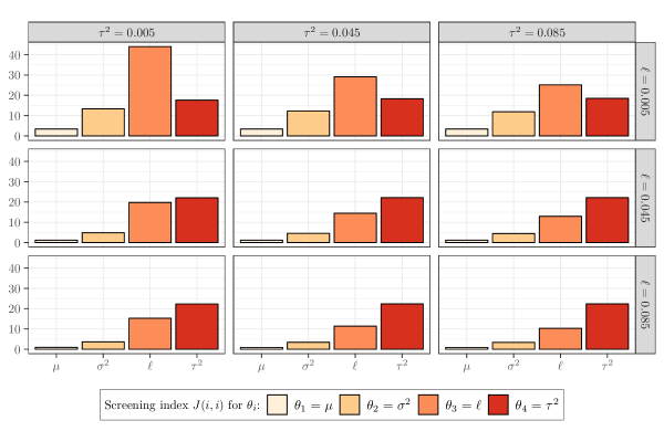
Recall that $\mathcal{S}$, defined in 21, is the sensitivity index based on the logarithmic derivative to control for differences in magnitude between the parameters. At present we assume that choice of solver is independent of the choice of parameters; in this case, the variance term of the marginal performance measure in 22 is fixed and the sensitivity of parameters can be screened based on the appropriately scaled FIM appearing in 22. In general, the solver and hence $\nu$ might depend on the parameters as these affect the regularity of the random field. In Figure 4, the screening index,

(24) $$J(i,i)=\theta_{i}\sqrt{v_{i}^{\top}\mathcal{I}(\theta)v_{i}},$$

is calculated for each $i=1,\dots,4$, that is for each of the principal parameter directions $\{\mu,\sigma^{2},\ell,\tau^{2}\}$ corresponding to the diagonals of the FIM. These indices are compared across a range of nominal models for a fixed goal functional. Figure 4 demonstrates the relative insensitivity of perturbations in $\mu$ and $\sigma^{2}$ over the range of nominal models where $\ell$ and $\tau^{2}$ vary for $\mu=0.8$ and $\sigma^{2}=4$. $J$ is computed without sampling using expression 23 and identifies that the directions $\mu$ and $\sigma^{2}$ might be excluded from the full sensitivity analysis for the given goal functional since the screening index is small relative to the value for other directions.

Figure 4. The screening index $J$ in 24 for the logarithmic-derivative based parametric sensitivity depends on the FIM and can be computed cheaply (without sampling) thus providing an efficient method for screening parameters. In this instance, $J$ indicates the directions $\mu$ and $\sigma^{2}$ are relatively insensitive compared to perturbations in $\ell$ and $\tau^{2}$ over nine different nominal models for a fixed QoI corresponding to a failure probability.

3.3. Robust bounds and worst-case scenarios

Next, we demonstrate bounds based on 12 in Theorem 1 that are more accurate than the linearized bounds at the cost of being more computationally expensive. To investigate the performance for parametric sensitivity analysis, we fix a nominal model $P^{\theta}$, with hyperparameters $\theta=(\mu=0.8,\sigma^{2}=4,\ell=0.005,\tau^{2}=0.045)$, and consider the sensitivity with respect to alternative models $P^{\theta+\epsilon v}$ corresponding to small perturbations in the $\ell$ and $\tau^{2}$ which we denote by $\epsilon(\ell)$ and $\epsilon(\tau^{2})$ (see also Figure 5c). We also fix the goal functionals

(25a) $$g_{1}(\bar{u})=\textbf{1}_{\{\bar{u}(1)>1.2\}}\,,$$

(25b) $$g_{2}(\bar{u})=\textbf{1}_{\{0.25<\bar{u}(1)<0.75\}}\,,\quad\text{and}$$

(25c) $$g_{3}(\bar{u})=\min(u(1),3)\,.$$

25a and 25b are indicator functions (QoI corresponding to failure probabilities cf. Theorem 2) and 25c is a point estimate with an enforced upper bound.

In Figures 5a and 5b, a scaled hybrid information divergence 11

(26) $$\frac{\theta}{\epsilon}\,\Xi_{\pm}(\gamma^{\prime}\mid\gamma;H^{g_{i}}),$$

is compared to the reference quantity,

(27) $$\hat{\Delta}(\epsilon,M;g_{i})=\frac{\theta}{\epsilon}\left(E_{\gamma^{\prime}}^{M}[g_{i}]-E_{\gamma}^{M}[g_{i}]\right),$$

a finite difference approximation of the sensitivity $\mathcal{S}$ where

(28) $$E_{\gamma}^{M}(f)=\frac{1}{M}\sum_{j=1}^{M}f(\omega_{j})$$

denotes the sample average based on $M$ independent and identically distributed samples of $f$ drawn with respect to $\gamma$. Each observation appearing in Figures 5a and 5b is based on the mean of ${10}^{2}$ runs of $M=${10}^{3}$$ samples and the confidence intervals denote two standard deviations from the corresponding sample mean.

(a)

(b)

(c)

Figure 5. In (a) and (b), the bounds 26 provide a tight estimate of the logarithmic-derivative based parametric sensitivity index 27 for bounded goal functionals 25a, 25b and 25c. The shaded regions in Figure 5a and Figure 5b denote confidence intervals of two standard deviations from the corresponding sample mean 28 based on $10^{2}$ runs of $M=10^{3}$ samples. Comparing (a) to (b) we observe that the bounds in (b) are captured by the corresponding bounds in (a); the relative entropy landscape in (c) reveals an explanation, namely, that the information budget established by $\epsilon(\ell)$, i.e. small $\epsilon$ perturbations in $\ell$, contains corresponding perturbations $\epsilon(\tau^{2})$. Thus, we note the bounds 26 in (a) are robust, providing a worst-case scenario envelope for all perturbations within an information budget (cf. Corollary 1).

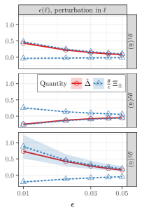
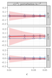
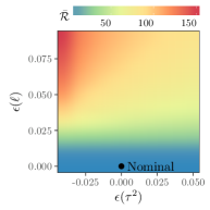
We observe in Figures 5a and 5b that for each QoI (facet corresponding to rows), the bounds 26 provide an accurate estimate of the sensitivity for $\epsilon(\ell)$ and $\epsilon(\tau^{2})$. In particular, the plots are suggestive of the tightness of the bounds derived from the hybrid information divergence. Further, a comparison of Figure 5a to Figure 5b, indicates that the bounds 26 are robust. For this particular nominal model, the relative entropy landscape in Figure 5c shows that $\epsilon(\tau^{2})$ always fall within the information budget established by $\epsilon(\ell)$, that is, the level sets relating to $\epsilon(\ell)$ contain the corresponding $\epsilon(\tau^{2})$. Thus, the bounds 26 in Figure 5a are guaranteed to contain the bounds in Figure 5b by Corollary 1 and can be interpreted as giving the worst-case scenario for each QoI, providing a natural way to rigorously incorporate worst-case scenarios into the decision support framework in Figure 1.

3.4. A posteriori computability

We emphasize that the components appearing in the argument of the optimization problem in 11, and in particular in the right-hand side of 26, are a posteriori computable quantities that represent significant computational savings over gradient approximations. Moreover, 26 incorporate worst-case scenarios that might not be efficiently observed using traditional estimates of the sensitivity. In the previous numerical experiment, we approximate 26 by

$$\Xi_{\pm}(\gamma^{\prime}\mid\gamma;H^{g})\approx\pm\xi(c^{*},\pm H^{g})$$

where $c^{*}=\operatorname{arg\,min}_{c>0}\xi(c,H^{g})$ and

(29) $$\xi(c,H^{g}):=\hat{\Lambda}_{\gamma}(c,H^{g})+\frac{1}{c}\bar{\operatorname{\mathcal{R}}}(\gamma^{\prime}\mid\gamma)$$

for suitable approximations $\hat{\Lambda}_{\gamma}$ and $\bar{\operatorname{\mathcal{R}}}$ of the risk-sensitive performance measure and relative entropy, respectively. The optimal $c^{*}$ as a function of $\rho:=\operatorname{\mathcal{R}}(\lambda\mid\gamma)$ has the representation

(30) $$c^{*}(\rho)=\frac{\sqrt{2\rho}}{\sqrt{\operatorname{Var}_{\gamma}[H^{g}]}}+O(\rho),$$

which follows from equation (2.28) of [21]. For perturbations resulting in small $\rho$ 30 can be used; otherwise, we find the optimal $c^{*}$ by a one-dimensional Newton-Raphson method, a step that must be repeated for each QoI for every alternative model under consideration.

The $\hat{\Lambda}_{\gamma}$ appearing in 29 can be sampled using a standard MC approximation,

$$\hat{\Lambda}_{\gamma}(c,H^{g})=\frac{1}{c}\log E_{\gamma}^{M}(\exp\{c(H^{g}-\widehat{H^{g}})\})\approx\Lambda_{\gamma}(c,H^{g}),$$

for $\widehat{H^{g}}:=E_{\gamma}^{M}(H^{g})\approx\operatorname{\mathbf{E}}_{\gamma}[H^{g}]$ where $E_{\gamma}^{M}$ denotes the sample average 28. This quantity needs to be computed only once for each QoI, according to the nominal model $\gamma$, and can then be used as in 17 to test any number of alternative models within the established information budget as in Corollary 1. In contrast, the relative entropy appearing in 29 needs to be computed for every alternative model under consideration. However, the relative entropy can be computed without sampling using the analytic formula 9 together with Remark 1 to replace the distribution of the conductivity with the corresponding Gaussian. In the preceding experiments the approximation $\bar{\operatorname{\mathcal{R}}}(\gamma^{\prime}\mid\gamma)\approx\operatorname{\mathcal{R}}(\gamma^{\prime}\mid\gamma)$ is obtained by taking the Gaussians to have the same dimension as the finite element discretization.

Remark 2:

Forming an estimator involving the hybrid information divergence $\Xi$ as in 26 requires sampling a cumulant generating functional ($\hat{\Lambda}_{\gamma}$). Although sampled with respect to the nominal model, if the variance of the marginal performance measure is large then this variance could potentially be amplified by $\hat{\Lambda}_{\gamma}$; in Figure 5a, the estimator of $\Xi_{+}$ for goal functional $g_{3}$ 25c is observed to have higher variance than the indicator functionals 25a and 25b. In section 5, we demonstrate concentration inequality bounds for $\Lambda_{\gamma}$ that results in reduced variance predictions the information divergences $\Xi_{\pm}$.

Remark 3:

The formula 9 depends on the discrete projection $(\bar{a}_{n})\approx a$. In some instances $\Sigma$ may be close to singular, hampering the computation of the precision matrix $\Sigma^{-1}$ or the $\log$-determinant. In the numerical experiments presented here, such issues were easily addressed using a Cholesky-like covariance decomposition and facts about Toeplitz matrices. Geostatistical models based on Markov random fields ([53]), as opposed to parametric covariance models, is an approach that sidesteps this difficulty and we note the techniques outlined here also apply to conductivities given by Markov random fields (see [32]).

In the next section, we examine non-parametric perturbations to a geostatistical model. In particular, Theorem 1 yields tight and robust UQ bounds in the context of model misspecification due to sparse data.

4. Data-informed error bounds for non-parametric perturbations

In the present section, we consider model-form uncertainty in connection with misspecification of the geostatistical model due to lacking or incomplete data. As emphasized in the introduction, data for our applications of interest are sparse and small perturbations to data result in geostatistical models that are non-parametric perturbations of the nominal model (see Figure 3). By allowing us to compare the effect that distributional assumptions on model inputs have on model outputs, the hybrid information divergence provides a link between data and decision tasks. In this vein, we explore how the hybrid information divergences complement an existing inference procedure by providing robust, data-informed bounds that give a sense of worst-case scenarios under modeling errors. Next, we review the data set and the inference procedure used in our experiments.

4.1. Conductivity data and model problem

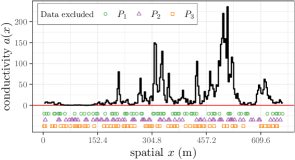
We utilize permeability data for a Brent sequence ($365.76\text{\,}\mathrm{m}$ by $670.56\text{\,}\mathrm{m}$ by $51.816\text{\,}\mathrm{m}$) from SPE10 model 2 in [12]. Due to its importance in the North Sea petroleum industry, the Brent sequence is well studied from a geological perspective ([51]). The sequence has two distinct phases; the upper layers of the sequence comprise a Tarbert formation and the bottom layers comprise an Upper Ness formation. The log-permeability of these two formations both vary by several orders of magnitude and exhibit strikingly different spatial correlations. In our numerical experiments, we will fit various geostatistical models based on data from a one-dimensional slice of the upper-most level of the Tarbert formation displayed in Figure 6a.

(a)

(b)

Figure 6. In (a), a one-dimensional slice of the Tarbert formation data (from SPE10 model 2 in [12]) used in numerical experiments in section 4 varies by orders of magnitude over the problem scale. In (b), three frequency distributions for the relative entropy are depicted for non-small perturbations of three different nominal models corresponding to $P_{1}$, $P_{2}$ and $P_{3}$ in (a). We observe that relative entropy distributions with respect to the family of alternative models 33 are multi-modal and depend in a nontrivial fashion on the nominal model (cf. the relative entropy landscape in Figure 5c where the small parametric perturbations result in a relatively flat landscape in the $\epsilon(\tau^{2})$ direction with a smooth ascent in $\epsilon(\ell)$).

For the experiments that follow, we fix both a parametric form for the geostatistical model and an inference procedure. We then consider different geostatistical models fit from incomplete samples of the full data set. Specifically, we assume that the available log-data are Gaussian and then fit the parameters of the geostatistical model using the maximum likelihood method. For a given parametric model, this method gives parameter values that are found to maximize the likelihood of making an observation of a particular data point given the parameter value; this process is entirely automated by a number of software packages and the present experiments use ‘RandomFields’ ([54]) available in R. For convenience we shall again use the covariance 20 from section 3. Although we posit a parametric form, geostatistical models resulting from fits relying on incomplete observations of the full data set are not in general small parametric perturbations of one another. Even small changes to these discrete degrees of freedom may result in global changes to parameters and hyperparameters, in contrast to the localized sensitivity analysis in section 3.

We again consider the one-dimensional model problem 19, where the conductivity fields $(\bar{a}_{n})$ are generated on a regular uniform mesh of $n$ equally spaced cells and this projection is used in forming the stiffness matrix for the FEM computation as well as the covariance matrices required for the relative entropy calculations (i.e. $n=d$). The FEM solution $(\bar{u}_{2n})$ is then computed using standard, piecewise linear elements on a coarse mesh with diameter $2n$.

In the remainder of the present section, we describe two numerical experiments that use the hybrid information divergence 12 to obtain data-informed bounds. The first experiment in section 4.2 provides a sense of the modeling error due to misspecification stemming from incomplete data over a range of changes to the discrete degrees of freedom. In the second experiment in section 4.3, we fix a nominal model based on a portion of the full data set and examine the distribution of the relative entropy to identify an information budget such that the hybrid information divergences give robust bounds that include worst-case scenarios.

4.2. Hybrid information divergences for model misspecification

In Figures 7 and 8, we demonstrate the sensitivity of the modeling error 3 with respect to changes in the geostatistical model resulting from the inclusion or exclusion of a small number of data points. This sensitivity is with respect to discrete changes to the degrees of freedom used to fit the parametric model and is not understood in the same sense as 21. The weak errors in Figures 7 and 8 are between a nominal model, based on a portion of the available data set, and alternative models that correspond to including or excluding a fixed number of points from the data used to construct the nominal model. The data-informed bounds derived from the hybrid information divergence give tight and robust predictions for this weak error.

Figure 7. For the failure probability goal functionals 32a and 32b, the data-informed bounds $\Xi_{\pm}$ 31 give a tight and robust prediction of the weak error $\mathcal{E}$ 3 over a range of changes to the discrete degrees of freedom. In (a) and (b) above, box plots are given for ${10}^{2}$ observations, each of $M=${10}^{3}$$, samples where trend lines through the mean are added to indicate how the bounds form an envelope around model predictions.

Figure 8. The data-informed bounds $\Xi_{\pm}$ 31 provide a tight and robust estimate of the weak error $\mathcal{E}$ 3 for an unbounded $g_{3}$ 32c, however $\Xi_{+}$ have high variance (cf. Remark 2). We emphasize that the predictions here and in Figure 7 are robust in that $\Xi_{\pm}$ bound the weak error for all alternative models that fall within a given information budget thus including a sense of worst-case scenarios. Above, box plots are given for ${10}^{2}$ observations, each of $M=${10}^{3}$$, samples where trend lines through the mean are added to indicate how the bounds form an envelope around model predictions.

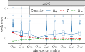
In particular, we begin by fixing a data set for the nominal model $\gamma$ by sampling, uniformly at random, $50$ percent of the full data set depicted in Figure 6a. We then fit a squared exponential covariance model 20 using the maximum likelihood method. We also fit a collection of alternative models $\{\lambda_{10},\dots,\lambda_{100}\}$ where $\lambda_{q}$ is related to a geostatistical model that is fit using $q$ percent of the full data set where a small number of points are added or deleted from the subset of data used for neighboring alternative models. For example, the data set used to construct $\lambda_{60}$ is formed by sampling $10$ percent of the data points from the full data set not included in $\lambda_{50}$ and then adding them to the partial set used for $\lambda_{50}$. In keeping with the notation used in previous sections, we then denote the nominal product measure $P=\gamma\otimes\nu$ and the alternatives $Q_{q}=\lambda_{q}\otimes\nu$. Thus, the weak error displayed in Figures 7 and 8 correspond to alternative models related to a perturbation of the observed data set used to fit the models, that is, to a perturbation of discrete degrees of freedom.

For this collection of nominal and alternative geostatistical models, the bounds

(31) $$\Xi_{\pm}(\lambda_{q}\mid\gamma;H^{g})\approx\pm\xi(c^{*},\pm H^{g})$$

are computed using an expression similar to 29 in the spirit of section 3.4. Box plots for ${10}^{2}$ observations of each bound and weak error, each based on $M=${10}^{3}$$ samples, are displayed in Figures 7 and 8 along with a trend line corresponding to the mean of the observations. The bounds and the weak errors are examined for the goal functionals,

(32a) $$g_{1}(\bar{u})=\textbf{1}_{\{\bar{u}(x_{1})>m\}}\,,$$

(32b) $$g_{2}(\bar{u})=\textbf{1}_{\{m+s>\bar{u}(x_{1})>m-s\}}\,,\quad\text{and}$$

(32c) $$g_{3}(\bar{u})=\bar{u}(x_{1})/m\,,$$

where $m$ is the sample average of $\bar{u}(x_{1})$ at the right-hand endpoint of the domain and $s$ is the corresponding standard deviation. We note that for 32a and 32b the weak error is bounded in $[-1,1]$ whereas for 32c it is unbounded and we therefore anticipate any estimate related to 32c to naturally have higher variance.

In Figure 7, related to 32a and 32b, we observe that there is a fairly wide spread in the values for the weak errors corresponding to different alternative models. In this instance, the data-informed bounds 31 form a tight envelope around this spread. Even in the case of 32c, Figure 8 illustrates that 31 gives a reliable estimate of the weak error. However, we observe that the estimator for $\Xi_{+}$ has high variance in this instance due to sampling strategy used for the risk-sensitive performance measure $\hat{\Lambda}_{\gamma}$. As noted in as in Remark 2, an alternative method will be discussed in section 5.

4.3. Finding worst-case scenarios related to incomplete data

Presently we examine worst-case scenarios due to changes in the discrete degrees of freedom. The distribution of the relative entropy with respect to a training set is used to determine an information budget that yields robust, data-informed bounds encapsulating worst-case scenarios.

Figure 9. Choosing an alternative model $Q_{\max}$ related to the maximum relative entropy observed in a training set yields robust, data-informed bounds $\Xi_{\pm}$ that include a sense of worst-case scenarios related to the impact of incomplete data on the modeling process for the nominal models $P_{1}$, $P_{2}$, and $P_{3}$ in Figure 6. The matrix of plots above contains box plots of ${10}^{2}$ observations, each of $M=${10}^{3}$$ samples, where trend lines through the means have been added to indicate how the bounds form an envelope around model predictions.

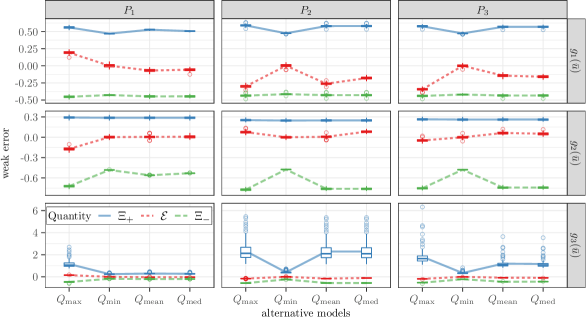
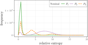
We consider three different nominal models, $P_{1}=\gamma_{1}\otimes\nu$, $P_{2}=\gamma_{2}\otimes\nu$, and $P_{3}=\gamma_{3}\otimes\nu$, that are related to fitting a parametric geostatistical model $\gamma_{i}$ to $70$ percent of the full data set sampled uniformly. In Figure 6a, the full data set is displayed in addition to the corresponding “gaps” in the three different nominal models. As in previous sections, these models are fit to a squared exponential covariance model 20 using the maximum likelihood method. For each nominal model, we build the training set

(33) $$\mathcal{Q}_{i}=\{Q^{+}=\lambda^{+}\otimes\nu\}\,,\quad i=1,2,3\,,$$

a collection of alternative models based on $\lambda^{+}$ that are fit to enlargements of the nominal model data (i.e. to $80$ percent of the full data set) where points are added by sampling those excluded from the nominal model set uniformly. The corresponding frequency distribution of the relative entropy for each $P_{i}$ with respect to $|\mathcal{Q}_{i}|=${10}^{5}$$ alternative models is displayed in Figure 6b. The distributions, which exhibit multi-modality, demonstrate the non-trivial dependence of the relative entropy on the nominal model under consideration. These frequency distributions play a similar role to the relative entropy landscape in Figure 5c since in this case there is no natural ordering among the alternative models (cf. Figure 5c where the small epsilon perturbation provides a basis for ordering the models). The tightness of the hybrid information divergence suggests that the modeling error 3 may cluster according to the peaks in the relative entropy distribution. Further, the information budget established by the maximum observed relative entropy can be used to bound all the alternative models in $\mathcal{Q}_{i}$ according to Corollary 1.

From each $\mathcal{Q}_{i}$, we select four alternative models $Q_{\max}=\lambda_{\max}\otimes\nu$, $Q_{\min}=\lambda_{\min}\otimes\nu$, $Q_{\mathrm{mean}}=\lambda_{\mathrm{mean}}\otimes\nu$, and $Q_{\mathrm{med}}=\lambda_{\mathrm{med}}\otimes\nu$ that correspond to the maximum, minimum, mean, and median relative entropy with respect to $P_{i}$, respectively, see also Figure 6b. In Figure 9, we observe that once again that the bounds $\Xi_{\pm}$ yield robust predictions for the modeling error between the nominal and each of the alternative models. As expected, we observe that the weak error corresponding to $Q_{\max}$ appear to be worst-case scenarios and that this error is reliably contained in the envelope defined by $\Xi_{\pm}$. In the present setting, these goal-oriented bounds $\Xi_{\pm}$ represent data-informed quantities that encapsulate worst-case scenarios for the errors in misspecifying the geostatistical model due to epistemic uncertainty.

5. Efficient computation of hybrid information divergences

The variance of the hybrid information divergence $\Xi$ depends on the variance of the risk-sensitive hybrid performance measure $\Lambda_{\gamma}(c,H^{g})$ defined in 10. As $\Lambda_{\gamma}$ has the form of a cumulant generating functional of the marginal performance measure $H^{g}$ in 8, the variance of $\Lambda_{\gamma}$ behaves like the variance of an exponential function of the random variable $H^{g}$. If $\Xi$ exhibits large variance, as observed for the upper bound $\Xi_{+}$ for the goal function $g_{3}$ in Figures 5a, 8 and 9, then attempting to reduce the overall variance by running additional simulations for $H^{g}$ may be infeasible if the solver for the forward model is computationally expensive. Presently, we outline a different strategy that involves estimating $\Lambda_{\gamma}$ by concentration inequalities from Large Deviations Theory ([7]). This approach was recently introduced and applied to model problems in [32] and we extend these ideas to complex systems involving random PDE where the stochastic fields are infinite dimensional and inferred from real-world data. The concentration inequality estimates that we explore rely on statistics of $H^{g}$, such as mean and variance, and provide a bound on $\Lambda_{\gamma}$, that can be used as a surrogate in $\Xi$, accounting for any available data. Thus, not only are these concentration inequality estimates computationally non-intrusive but they also rely on quantities that one is already likely to compute in the normal course of a simulation.

5.1. Variance of the standard estimator for $\Xi$

The variance of the standard MC estimator for $\Xi_{+}$ is given by

$$\operatorname{Var}_{\gamma}\left[\Xi_{+}(\lambda\mid\gamma;H^{g})\right]=\frac{\operatorname{Var}_{\gamma}[e^{c^{*}H^{g}}]}{(c^{*})^{2}M(\operatorname{\mathbf{E}}_{\gamma}[e^{c^{*}H^{g}}])^{2}},$$

a quantity that depends exponentially on both $c^{*}$ and $H^{g}$. We recall that the optimal $c^{*}$ is linked to the information budget $\rho=\operatorname{\mathcal{R}}(\lambda\mid\gamma)$ by (30). For alternative models that are close in relative entropy to the nominal model, such as small parametric perturbations, then 30 provides a good approximation of the optimal $c^{*}$ up to first order in $\rho$. However, for alternative models that are a large relative entropy distance from the nominal model, we see from 30 that the optimal $c^{*}$ grows at least linearly in $\rho$.

Attempting to sample an estimator with large variance poses a difficulty for the present application of interest as sampling involves calls to a random PDE solver. In such settings, it is therefore of interest to find an alternative strategy to sampling $\Lambda_{\gamma}$. As suggested by the right-hand side of 10, $\Lambda_{\gamma}$ may have a known description as a cumulant generating functional for particular $H^{g}$. In other instances, $\gamma$ might have a form amenable to the numerical integration of $\operatorname{\mathbf{E}}_{\gamma}[e^{c(H^{g}-\operatorname{\mathbf{E}}_{\gamma}[H^{g}])}]$, for example via thermodynamic integration techniques ([40]).

In the remainder of this section, we indicate an alternative approach, recently introduced in [32], that relies on concentration inequalities from large deviations theory to bound $\Lambda_{\gamma}$. The concentration inequalities, at least in their simplest form, require bounded observables $H^{g}$ but rely on quantities that we are already likely to be sampling in our simulation such as the expected value and the variance. Although in the form of concentration inequalities discussed below the observable must be bounded, we show that such bounds produce fairly reliable results even when the observable is merely finite and an artificial bound is imposed (see Remark 4). We refer to [32] for a complete discussion on UQ methods based on concentration inequalities for both bounded and unbounded observables in several model problems.

5.2. Concentration inequalities for risk-sensitive performance measures

We recall the following bound on the moment generating function of a random variable in terms of its first two moments (see e.g. [17]).

Lemma 2 (Bennett).

Supposed $X\leq b$ is a real-valued random variable with $m=\operatorname{\mathbf{E}}[X]$ and $\operatorname{\mathbf{E}}[(X-m)^{2}]\leq s^{2}$ for some $s>0$. Then, for any $c\geq 0$,

$$\operatorname{\mathbf{E}}[e^{cX}]\leq e^{cm}\left(\frac{(b-m)^{2}}{(b-m)^{2}+s^{2}}e^{-\frac{cs^{2}}{b-m}}+\frac{s^{2}}{(b-m)^{2}+s^{2}}e^{c(b-m)}\right).$$

Thus we formulate a bound for $\Lambda_{\gamma}(c,H^{g})$ where the estimator of this quantity does not involve sampling an exponentially large quantity, i.e. the moment generating functional.

Theorem 3 (Concentration).

For a bounded observable $H^{g}\leq\bar{b}$ and $c\geq 0$,

$$\Lambda_{\gamma}(c,H^{g})\leq\frac{1}{c}\log\left(\frac{(\bar{b}-\widehat{H^{g}})^{2}}{(\bar{b}-\widehat{H^{g}})^{2}+s_{g}^{2}}e^{-cs_{g}^{2}/(\bar{b}-\widehat{H^{g}})}+\frac{s_{g}^{2}}{(\bar{b}-\widehat{H^{g}})^{2}+s_{g}^{2}}e^{c(\bar{b}-\widehat{H^{g}})}\right),$$

where $\widehat{H^{g}}=\operatorname{\mathbf{E}}_{\gamma}[H^{g}]$ and $s_{g}^{2}=\operatorname{Var}_{\gamma}[H^{g}]$.

Proof.

This follows immediately from Lemma 2 by considering the centered $X=H^{g}-\widehat{H^{g}}$ with $b=\bar{b}-\widehat{H^{g}}$, $m=\operatorname{\mathbf{E}}[H^{g}-\widehat{H^{g}}]=0$, and $s_{g}^{2}=\operatorname{\mathbf{E}}[X^{2}]=\operatorname{Var}_{\gamma}[H^{g}]$. ∎

We note from Theorem 2, that for failure probabilities the risk-sensitive performance measure has the form 18 thus the bound appearing in Theorem 3 holds with equality. An immediate extension to Lemma 2 bounds the moment generating function in terms of its mean and support and can be used when $H^{g}$ has both an upper and lower bound.

Lemma 3 (Bennett-$(a,b)$).

Suppose $X\in[a,b]$, for fixed $a<b$, is a real-valued random variable with $m=\operatorname{\mathbf{E}}[X]$. Then for any $c\in\textbf{R}$,

$$\operatorname{\mathbf{E}}[e^{cX}]\leq\frac{m-a}{b-a}e^{cb}+\frac{b-m}{b-a}e^{ca}.$$

We end by demonstrating these alternative bounds for the experiment in section 3.

5.3. Implementation for a parametric model

In the spirit of 29, we let

(34) $$\zeta(c,H^{g}):=\bar{\Lambda}_{\gamma}(c,H^{g})+\frac{1}{c}\bar{\operatorname{\mathcal{R}}}(\gamma^{\prime}\mid\gamma),$$

and obtain

(35) $$B_{+}(H^{g})\approx\zeta(c^{*},H^{g})\qquad\text{and}\qquad C_{+}(H^{g})\approx\zeta(c^{*},H^{g}),$$

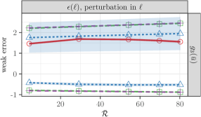
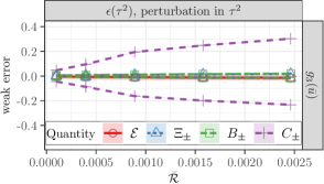
for an optimal $c^{*}$ where $\bar{\Lambda}_{\gamma}(c,H^{g})$ in 34 is approximated using Theorem 3 and Lemma 3, respectively. These surrogates for the cumulant generating functional account for any available data through suitable statistical quantities of the marginal performance measure $H^{g}$ in 8 that is related to the propagation of model-form uncertainty from the geostatistical model to the forward model in Figure 1. Corresponding lower bounds, $B_{-}(H^{g})$ and $C_{-}(H^{g})$, are derived in a similar manner. In Figure 10, we demonstrate all of the bounds for the goal functional $g_{3}$ 32c, noting that the bounds $B_{\pm}$ and $C_{\pm}$ have much smaller variance than the estimator for $\Xi_{\pm}$ and in each case form an envelope around the sensitivity for the QoI that remains tight and robust. In Figure 10, the shaded regions denoting confidence intervals for the concentration inequalities $B_{\pm}$ and $C_{\pm}$ are negligible compared to the shaded region for the estimator of $\Xi_{\pm}$. The smaller variance of the concentration inequalities comes at the cost of some tightness in the estimates for $\mathcal{E}$.

(a)

(b)

Figure 10. The bounds $\Xi_{\pm}$, $B_{\pm}$, and $C_{\pm}$ are compared above for predictions of the weak error $\mathcal{E}$ between small parametric perturbations of $\ell$ (a) and $\tau^{2}$ (b) for the parametric geostatistical model with mean $\mu$ and covariance 20 (cf. Figures 5a and 5b). The bounds $B_{\pm}$ and $C_{\pm}$ in 35 based on the Bennett and Bennett-$(a,b)$ concentration inequalities in Lemmas 2 and 3 provide a computationally efficient alternative to sampling the cumulant generating functional for the marginal performance measure directly when the goal functional has high variance as is the case for 32c. Notice in (a) that the shaded regions denoting confidence intervals for the concentration inequalities $B_{\pm}$ and $C_{\pm}$ are negligible compared to shaded region for the estimator of $\Xi_{\pm}$. The smaller variance of the concentration inequalities comes at the cost of some tightness in the estimates for $\mathcal{E}$; in this case $\Xi\leq B_{\pm}\leq C_{\pm}$. In particular, we observe in (b) that $C_{\pm}$ over predicts the weak error $\mathcal{E}$.

Remark 4:

Although the concentration inequalities as quoted here are indicated only for a bounded QoI, we note that there exist other formulations for unbounded QoIs such as for sub-Gaussian random variables ([32]). In practice Theorem 3 is a useful computational tool for a finite QoI; we observe the tight bounds demonstrated in Figure 10 are for $g_{3}(\bar{u})=\min(\bar{u}(1),3)$ where the cut-off was arbitrarily chosen using a training set of ${10}^{3}$ observations of $\bar{u}(1)$.

6. Conclusions

The present work develops UQ tools for a random PDE model of steady-state subsurface flow in Figure 1 with potential impacts in hydrology, carbon sequestration, and petroleum engineering. These tools are realized through the novel application of hybrid information divergences that balance observable and data dependent quantities. The hybrid nature of the divergences allows us to represent and distinguish various sources of uncertainty entering into the model by attaching different levels of confidence to parts of the model. Ultimately, this allows us to address a key challenge concerning the propagation of model-form or epistemic uncertainty from the geostatistical model via the pathway in Figure 2.

We derive tight and robust estimates for modeling errors or biases from the hybrid information divergences and apply these to important UQ tasks including parametric sensitivity analysis and model misspecification arising from sparse data. In particular, we demonstrate the use of these bounds for making data-informed predictions such as quantifying the impact of incomplete data as in section 4. The robustness, when interpreted as including worst-case scenarios within a given information budget (i.e. within a family of acceptable alternative models, see Figure 3), suggests that these bounds are an appropriate deliverable in the context of the decision support framework in Figure 1. We emphasize that the bounds derived here are also goal-oriented and non-intrusive in nature, that is, can be used in conjunction with any algorithm or solver for the random PDE problem in Figure 1. Finally, we also make connections between the hybrid information divergences and certain concentration inequalities from Large Deviations Theory that can be leveraged for efficient computing and account for any available data through suitable statistical quantities.

Appendix A Source code

Source code and links to observational data are available at
https://github.com/ejhall/robust-uq-divergences.

References

- [1] J. r. E. Aarnes, K.-A. Lie, V. Kippe, and S. Krogstad, Multiscale methods for subsurface flow, in Multiscale Modeling and Simulation in Science, B. Engquist, P. Löstedt, and O. Runborg, eds., vol. 66, Springer, Berlin, 2009, pp. 3–48, https://doi.org/10.1007/978-3-540-88857-4_1.
- [2] M. P. Anderson, W. W. Woessner, and R. J. Hunt, Applied Groundwater Modeling: Simulation of Flow and Advective Transport, Academic Press, 2015, https://doi.org/10.1016/B978-0-08-091638-5.00013-4.
- [3] G. Arampatzis, M. A. Katsoulakis, and Y. Pantazis, Accelerated sensitivity analysis in high-dimensional stochastic reaction networks, PLoS ONE, 10 (2015), e0130825, https://doi.org/10.1371/journal.pone.0130825.
- [4] R. Atar, K. Chowdhary, and P. Dupuis, Robust bounds on risk-sensitive functionals via rényi divergence, SIAM/ASA J. Uncertain. Quantif., 3 (2015), pp. 18–33, https://doi.org/10.1137/130939730.
- [5] I. Babuška, F. Nobile, and R. Tempone, A stochastic collocation method for elliptic partial differential equations with random input data, SIAM J. Numer. Anal., 45 (2007), pp. 1005–1034, https://doi.org/10.1137/050645142.
- [6] A. Ben-Tal, L. El Ghaoui, and A. Nemirovski, Robust Optimization, Princeton Series in Applied Mathematics, Princeton University Press, October 2009, https://doi.org/10.1515/9781400831050.
- [7] S. Boucheron, G. Lugosi, and P. Massart, Concentration Inequalities: A Nonasymptotic Theory of Independence, Oxford University Press, 2013, https://doi.org/10.1093/acprof:oso/9780199535255.001.0001.
- [8] K. P. Burnham and D. R. Anderson, Model Selection and Multimodel Inference, Springer-Verlag, New York, second ed., 2002, https://doi.org/10.1007/b97636.
- [9] J. Charrier, Strong and weak error estimates for elliptic partial differential equations with random coefficients, SIAM J. Numer. Anal., 50 (2012), pp. 216–246, https://doi.org/10.1137/100800531.
- [10] J. Charrier, R. Scheichl, and A. L. Teckentrup, Finite element error analysis of elliptic PDEs with random coefficients and its application to multilevel Monte Carlo methods, SIAM J. Numer. Anal., 51 (2013), pp. 322–352, https://doi.org/10.1137/110853054.
- [11] K. Chowdhary and P. Dupuis, Distinguishing and integrating aleatoric and epistemic variation in uncertainty quantification, ESAIM Math. Model. Numer. Anal., 47 (2013), pp. 635–662, https://doi.org/10.1051/m2an/2012038.
- [12] M. Christie, M. Blunt, et al., Tenth SPE comparative solution project: A comparison of upscaling techniques, in SPE Reservoir Simulation Symposium, Society of Petroleum Engineers, 2001, https://doi.org/10.2118/72469-PA.
- [13] K. A. Cliffe, M. B. Giles, R. Scheichl, and A. L. Teckentrup, Multilevel Monte Carlo methods and applications to elliptic PDEs with random coefficients, Comput. Vis. Sci., 14 (2011), pp. 3–15, https://doi.org/10.1007/s00791-011-0160-x.
- [14] T. M. Cover and J. A. Thomas, Elements of Information Theory, Wiley-Interscience, Hoboken, NJ, second ed., 2006, https://doi.org/10.1002/047174882X.
- [15] G. Dagan, Statistical theory of groundwater flow and transport: Pore to laboratory, laboratory to formation, and formation to regional scale, Water Resources Research, 22 (1986), pp. 120S–134S, https://doi.org/10.1029/WR022i09Sp0120S.
- [16] G. Dagan, Flow and Transport in Porous Formations, Springer-Verlag, Berlin, 1989, https://doi.org/10.1007/978-3-642-75015-1.
- [17] A. Dembo and O. Zeitouni, Large Deviations Techniques and Applications, vol. 38 of Stochastic Modelling and Applied Probability, Springer-Verlag, Berlin, 2010, https://doi.org/10.1007/978-3-642-03311-7.
- [18] J. E. Doherty and R. J. Hunt, Approaches to highly parameterized inversion: A guide to using PEST for model-parameter and predictive-uncertainty analysis, tech. report, US Geological Survey, 2010, http://pubs.usgs.gov/sir/2010/5211.
- [19] J. C. Duchi, M. I. Jordan, and M. J. Wainwright, Local privacy and statistical minimax rates, in 2013 IEEE 54th Annual Symposium on Foundations of Computer Science, Oct 2013, pp. 429–438, https://doi.org/10.1109/FOCS.2013.53.
- [20] P. Dupuis and R. S. Ellis, A Weak Convergence Approach to the Theory of Large Deviations, John Wiley & Sons, New York, 1997, https://doi.org/10.1002/9781118165904.
- [21] P. Dupuis, M. A. Katsoulakis, Y. Pantazis, and P. Plecháč, Path-space information bounds for uncertainty quantification and sensitivity analysis of stochastic dynamics, SIAM/ASA J. Uncertain. Quantif., 4 (2016), pp. 80–111, https://doi.org/10.1137/15M1025645.
- [22] W. Durner, Hydraulic conductivity estimation for soils with heterogeneous pore structure, Water Resour. Res., 30 (1994), pp. 211–223, https://doi.org/10.1029/93WR02676.
- [23] R. S. Ellis, Entropy, Large Deviations, and Statistical Mechanics, Springer-Verlag, Berlin, 2006, https://doi.org/10.1007/3-540-29060-5, http://dx.doi.org/10.1007/3-540-29060-5.
- [24] O. G. Ernst, A. Mugler, H.-J. Starkloff, and E. Ullmann, On the convergence of generalized polynomial chaos expansions, ESAIM Math. Model. Numer. Anal., 46 (2012), pp. 317–339, https://doi.org/10.1051/m2an/2011045.
- [25] R. E. Ewing, ed., The Mathematics of Reservoir Simulation, vol. 1 of Frontiers in Applied Mathematics, SIAM, Philadelphia, PA, 1983, https://doi.org/10.1137/1.9781611971071.
- [26] S. Ferson and L. R. Ginzburg, Different methods are needed to propagate ignorance and variability, Reliab. Eng. Syst. Safe., 54 (1996), pp. 133–144, https://doi.org/http://dx.doi.org/10.1016/S0951-8320(96)00071-3.
- [27] A. E. Gelfand, P. J. Diggle, M. Fuentes, and P. Guttorp, eds., Handbook of Spatial Statistics, CRC Press, Boca Raton, FL, 2010, https://doi.org/10.1201/9781420072884.
- [28] M. Gil, F. Alajaji, and T. Linder, Rényi divergence measures for commonly used univariate continuous distributions, Inform. Sci., 249 (2013), pp. 124–131, https://doi.org/10.1016/j.ins.2013.06.018.
- [29] P. Glasserman, Monte Carlo Methods in Financial Engineering, vol. 53, Springer, New York, 2003, https://doi.org/10.1007/978-0-387-21617-1.
- [30] P. Glasserman and D. D. Yao, Some guidelines and guarantees for common random numbers, Management Science, 38 (1992), pp. 884–908, https://doi.org/10.1287/mnsc.38.6.884.
- [31] K. Gourgoulias, M. A. Katsoulakis, and L. Rey-Bellet, Information metrics for long-time errors in splitting schemes for stochastic dynamics and parallel kinetic monte carlo, SIAM J. Sci. Comput., 38 (2016), pp. A3808–A3832, https://doi.org/10.1137/15M1047271.
- [32] K. Gourgoulias, M. A. Katsoulakis, L. Rey-Bellet, and J. Wang, How biased is your model? Concentration inequalities, information and model bias. Sumbitted (arXiv:1706.10260), Jun 2017, https://arxiv.org/abs/1706.10260.
- [33] E. J. Hall, H. Hoel, M. Sandberg, A. Szepessy, and R. Tempone, Computable error estimates for finite element approximations of elliptic partial differential equations with rough stochastic data, SIAM J. Sci. Comput., 38 (2016), pp. A3773–A3807, https://doi.org/10.1137/15M1044266.
- [34] V. Harmandaris, E. Kalligiannaki, M. Katsoulakis, and P. Plecháč, Path-space variational inference for non-equilibrium coarse-grained systems, J. Comput. Phys., 314 (2016), pp. 355 – 383, https://doi.org/http://dx.doi.org/10.1016/j.jcp.2016.03.021.
- [35] J. C. Helton, Treatment of uncertainty in performance assessments for complex systems, Risk Anal., 14 (1994), pp. 483–511, https://doi.org/10.1111/j.1539-6924.1994.tb00266.x.
- [36] F. O. Hoffman and J. S. Hammonds, Propagation of uncertainty in risk assessments: The need to distinguish between uncertainty due to lack of knowledge and uncertainty due to variability, Risk Anal., 14 (1994), pp. 707–712, https://doi.org/10.1111/j.1539-6924.1994.tb00281.x.
- [37] S. C. Hora, Aleatory and epistemic uncertainty in probability elicitation with an example from hazardous waste management, Reliab. Eng. Syst. Safe., 54 (1996), pp. 217–223, https://doi.org/10.1016/S0951-8320(96)00077-4.
- [38] M. A. Katsoulakis, L. Rey-Bellet, and J. Wang, Scalable information inequalities for uncertainty quantification, J. Comput. Phys., 336 (2017), pp. 513 – 545, https://doi.org/10.1016/j.jcp.2017.02.020.
- [39] M. Komorowski, M. J. Costa, D. A. Rand, and M. P. Stumpf, Sensitivity, robustness, and identifiability in stochastic chemical kinetics models, Proc. Natl. Acad. Sci. USA, 108 (2011), pp. 8645–8650, https://doi.org/10.1073/pnas.1015814108.
- [40] T. Lelièvre, M. Rousset, and G. Stoltz, Free Energy Computations, Imperial College Press, London, 2010, https://doi.org/10.1142/9781848162488.
- [41] J. Li, X. Qi, and D. Xiu, On upper and lower bounds for quantity of interest in problems subject to epistemic uncertainty, SIAM J. Sci. Comput., 36 (2014), pp. A364–A376, https://doi.org/10.1137/120892969.
- [42] J. Li and D. Xiu, Computation of failure probability subject to epistemic uncertainty, SIAM J. Sci. Comput., 34 (2012), pp. A2946–A2964, https://doi.org/10.1137/120864155.
- [43] F. Liese and I. Vajda, Convex Statistical Distances, Teubner, Leipzig, 2007.
- [44] H. G. Matthies and A. Keese, Galerkin methods for linear and nonlinear elliptic stochastic partial differential equations, Comput. Methods Appl. Mech. Engrg., 194 (2005), pp. 1295–1331, https://doi.org/10.1016/j.cma.2004.05.027.
- [45] D. McLaughlin and L. R. Townley, A reassessment of the groundwater inverse problem, Water Resour. Res., 32 (1996), pp. 1131–1161, https://doi.org/10.1029/96WR00160.
- [46] W. L. Oberkampf, J. C. Helton, C. A. Joslyn, S. F. Wojtkiewicz, and S. Ferson, Challenge problems: Uncertainty in system response given uncertain parameters, Reliab. Eng. Syst. Safe., 85 (2004), pp. 11–19, https://doi.org/10.1016/j.ress.2004.03.002.
- [47] H. Owhadi, C. Scovel, T. J. Sullivan, M. McKerns, and M. Ortiz, Optimal uncertainty quantification, SIAM Review, 55 (2013), pp. 271–345, https://doi.org/10.1137/10080782X, https://doi.org/10.1137/10080782X, https://arxiv.org/abs/https://doi.org/10.1137/10080782X.
- [48] G. W. Parry, The characterization of uncertainty in probabilistic risk assessments of complex systems, Reliab. Eng. Syst. Safe., 54 (1996), pp. 119–126, https://doi.org/10.1016/S0951-8320(96)00069-5.
- [49] M. E. Paté-Cornell, Uncertainties in risk analysis: Six levels of treatment, Reliab. Eng. Syst. Safe., 54 (1996), pp. 9–111, https://doi.org/10.1016/S0951-8320(96)00067-1.
- [50] C. E. Rasmussen and C. K. I. Williams, Gaussian Processes for Machine Learning, MIT Press, Cambridge, MA, 2006, http://www.gaussianprocess.org/gpml/.
- [51] P. Richards, An introduction to the Brent Group: A literature review, in Geology of the Brent Group, A. Morton, R. Haszeldine, M. Giles, and S. Brown, eds., no. 61 in Special Publications, Geological Society of London, London, 1992, pp. 15–26, https://doi.org/10.1144/GSL.SP.1992.061.01.03.
- [52] W. D. Rowe, Understanding uncertainty, Risk Anal., 14 (1994), pp. 743–750, https://doi.org/10.1111/j.1539-6924.1994.tb00284.x.
- [53] H. Rue and L. Held, Gaussian Markov Random Fields, vol. 104 of Monographs on Statistics and Applied Probability, Chapman and Hall/CRC, Boca Raton, FL, 2005, https://doi.org/10.1201/9780203492024.
- [54] M. Schlather, A. Malinowski, M. Oesting, D. Boecker, K. Strokorb, S. Engelke, J. Martini, F. Ballani, O. Moreva, J. Auel, P. Menck, S. Gross, U. Ober, C. Berreth, K. Burmeister, J. Manitz, P. Ribeiro, R. Singleton, B. Pfaff, and R Core Team, Randomfields: Simulation and Analysis of Random Fields, 2017, https://cran.r-project.org/web/packages/RandomFields/index.html (accessed 2017-04-18). R package version 3.1.50.
- [55] D. M. Tartakovsky, Assessment and management of risk in subsurface hydrology: A review and perspective, Advances in Water Resources, 51 (2013), pp. 247–260, https://doi.org/10.1016/j.advwatres.2012.04.007.
- [56] A. Tsourtis, Y. Pantazis, M. A. Katsoulakis, and V. Harmandaris, Parametric sensitivity analysis for stochastic molecular systems using information theoretic metrics, J. Chem. Phys., 143 (2015), 014116, https://doi.org/10.1063/1.4922924.
- [57] A. B. Tsybakov, Introduction to Nonparametric Estimation, Springer Series in Statistics, Springer, New York, 2009, https://doi.org/10.1007/978-0-387-79052-7.
- [58] L. Wasserman, All of Statistics, Springer-Verlag, New York, 2004, https://doi.org/10.1007/978-0-387-21736-9.