Spin relaxation in disordered graphene:
Interplay between puddles and defect-induced magnetism

Abstract

We study the spin relaxation in graphene due to magnetic moments induced by defects. We propose and employ in our studies a microscopic model that describes magnetic impurity scattering processes mediated by charge puddles. This model incorporates the spin texture related to the defect-induced state. We calibrate our model parameters using experimentally-inferred values. The results we obtain for the spin relaxation times are in very good agreement with experimental findings. Our study leads to a comprehensive explanation for the short spin relaxation times reported in the experimental literature. We also propose a new interpretation for the puzzling experimental observation of enhanced spin relaxation times in hydrogenated graphene samples in terms of a combined effect due to disorder configurations that lead to an increased coupling to the magnetic moments and the tunability of the defect-induced $\pi$-like magnetism in graphene.

I Introduction

The spin properties of graphene Han et al. (2014); Roche and Valenzuela (2014); Pesin and MacDonald (2012); Soriano et al. (2015) are one of the many fascinating aspects of this material. The combination of carbon’s low atomic number and the planar structure of graphene’s lattice entails a very low intrinsic spin-orbit coupling, in the range of 1 $\mu$eV Han et al. (2014); Roche and Valenzuela (2014); Pesin and MacDonald (2012), and negligible hyperfine interactions. As a consequence, pioneering theoretical studies predicted that electrons could travel for long distances and long times in graphene without spin flipping Han et al. (2014); Roche and Valenzuela (2014); Pesin and MacDonald (2012). This property would make graphene a very interesting candidate for passive spintronics devices Han et al. (2014); Fabian et al. (2007); Žutić et al. (2004). However, since the first successful experimental demonstration of injection of a spin-polarized current in graphene Tombros et al. (2007), the measured spin relaxation times have been found to be orders of magnitude smaller than the theoretical predictions Han et al. (2014); Roche and Valenzuela (2014); Soriano et al. (2015). The small relaxation times observed in Ref. Tombros et al., 2007 were confirmed by other experiments with different setups Wojtaszek et al. (2013); Maassen et al. (2013); Omar et al. (2015); Balakrishnan et al. (2013); Han and Kawakami (2011); McCreary et al. (2012); Drogeler et al. (2016). A large theoretical effort has been devoted to unravel this puzzle Ertler et al. (2009); Ochoa et al. (2012); Fedorov et al. (2013); Tuan et al. (2014); Bundesmann et al. (2015); Huang et al. (2016); Kochan et al. (2014); Soriano et al. (2015); Wilhelm et al. (2015); Vierimaa et al. (2017); Van Tuan et al. (2016); Cummings and Roche (2016); Thomsen et al. (2015); Van Tuan and Roche (2016) and different mechanisms have been proposed for the enhanced spin relaxation, such as charge puddles Ertler et al. (2009); Van Tuan et al. (2016); Vierimaa et al. (2017), impurity-induced enhancement of spin orbit interaction Fedorov et al. (2013); Bundesmann et al. (2015); Tuan et al. (2014); Huang et al. (2016) and magnetic impurities Kochan et al. (2014); Soriano et al. (2015); Wilhelm et al. (2015); Vierimaa et al. (2017).

Light adatoms such as hydrogen and lattice defects (vacancies) have been proposed to give rise to $\pi-$like magnetism in graphene Yazyev and Helm (2007); Yazyev (2010). The origin of this kind of magnetism relies on the bipartite character of the lattice Yazyev (2010); Miranda et al. (2016) and on electron-electron interactions Lieb (1989). Whenever an imbalance between sublattices $A$ and $B$ occurs $N=|N_{A}-N_{B}|\neq 0$ zero modes appear Pereira et al. (2008); Inui et al. (1994), and upon the presence of electron-electron interactions the ground state of the system is magnetic with total spin $S=N/2$ Yazyev (2010); Lieb (1989). For the case of a single impurity, it has been shown theoretically that the magnetism is associated with the wave function of the zero mode, which extends over many lattice sites Yazyev (2010); Chang and Haas (2011); Nanda et al. (2012); Palacios et al. (2008); Kochan et al. (2014); Miranda et al. (2016). This magnetism is unusual since, ordinarily, magnetism is related to atoms with $d$ and $f$ unfilled shells and is very localized around such atoms. $\pi-$like induced magnetism due to hydrogen adatoms Gonzalez-Herrero et al. (2016) or vacancies Zhang et al. (2016) were reported recently in scanning tunneling microscopy experiments and the magnetic texture confirmed Gonzalez-Herrero et al. (2016).

Kochan and collaborators Kochan et al. (2014) proposed that magnetic impurities in graphene act as hot spots, flipping the spins of the electrons as they are scattered by these impurities. Small spin relaxation times have been measured in hydrogenated Wojtaszek et al. (2013); Balakrishnan et al. (2013); McCreary et al. (2012) samples and in graphene with vacancies McCreary et al. (2012). Although other mechanisms such as spin-orbit coupling are predicted to arise in hydrogenated graphene Castro Neto and Guinea (2009); Gmitra et al. (2013); Balakrishnan et al. (2013) and compete with the magnetic-induced spin flipping for fast spin relaxation, several studies point to the latter as the dominant mechanism in these systems Soriano et al. (2015); Bundesmann et al. (2015); Wilhelm et al. (2015).

It is difficult to capture the spatial texture of the impurity-induced magnetism in graphene with an effective impurity Hamiltonian. Previous studies made use of ab initio calculations to evaluate the microscopic structure of the system and extract the parameters of an effective impurity tight-binding Hamiltonian Gmitra et al. (2013); Kochan et al. (2014); Soriano et al. (2015); Thomsen et al. (2015). The pioneering approach developed by Kochan and collaborators Kochan et al. (2014) indicate that the largest contribution to spin-flip processes comes from the exchange term at the hydrogen site, justifying neglecting the contribution coming from farther sites. Although this simplification allows for an elegant analytical solution of the problem, it is not clear what are the effects of disregarding the extended character of the induced magnetism. The authors of Ref. Kochan et al., 2014 needed to perform an ad hoc convolution to treat the effect of electron-hole puddles when fitting their theory to the experimental data Kochan et al. (2014).

A very recent study Vierimaa et al. (2017) has shown that close to the Dirac point the energy dependence of the spin relaxation time has a strong reliance on the range of the magnetic impurities. This result points to the relevance of considering the extended nature of the magnetism induced by vacancies or hydrogen adatoms in graphene. Recently, two studies Soriano et al. (2015); Vierimaa et al. (2017) have proposed different models to treat spin-flip process due to magnetic impurities; however, the spatial range and modulation of the magnetic profile in these models was chosen arbitrarily.

In this paper we address the issue of spin relaxation in graphene due to magnetic moments induced by defects. We derive a comprehensive microscopic formalism that accounts for the interplay between local chemical potential fluctuations, which give rise to charge puddles, and magnetic impurities, and hence incorporates the spin texture related to the defect-induced state. In our model, the local chemical potential fluctuations not only modify the density of states close to the charge neutrality point, but also play a key role in the spin flip scattering mechanism. Our study leads to a novel, alternative explanation for the short spin relaxation times reported in experimental literature and sheds some light on the dominant mechanism of spin relaxation in hydrogenated graphene.

The paper is organized as follows: In Sec. II we introduce the tight-binding Hamiltonians we use to model vacancies and adatoms in graphene in the presence of disorder-induced charge puddles. Further, we present a microscopic derivation of the Anderson single impurity model and the spin relaxation times within this setting. In Sec. III we show the results of our simulations and analyze how the spin relaxation time $\tau_{s}$ depends on the model parameters. The technical details of the numerical procedure are discussed in the Appendix. We conclude in Sec. IV with a discussion of different scenarios to interpret the experimental results within realistic parameter choices.

II Theoretical approach

We study spin relaxation due to two kinds of defects that have been shown to induce magnetism in graphene, namely, vacancies and hydrogen adatoms. A single tight-binding model is usually employed to address both types of defects Yazyev and Helm (2007); Soriano et al. (2011, 2015). Here we treat the two cases separately, analyzing their similarities and differences.

Taking into account electron-electron interaction and long-range disorder, we map the model defect tight-binding Hamiltonian onto the single impurity Anderson model.

II.1 Mapping onto the Anderson Hamiltonian

To represent a vacancy, we adopt the standard $\pi$-band nearest-neighbor tight-binding Hamiltonian to describe the low-energy electronic properties of a graphene sheet,

$$H^{\rm vac}=-t\sum_{\langle i,j\rangle}|i\rangle\langle j|+t\sum_{\langle{\rm v},i\rangle}|{\rm v}\rangle\langle i|+\mbox{H.c.},$$ (1)

where $\langle\cdots\rangle$ restricts the sum over nearest-neighbor atomic sites and $t=2.8$ eV is the hopping matrix element between nearest neighbors. Notice that the second term on the right-hand side of Eq. (1) removes the defective (v site) from the honeycomb lattice.

Ab initio calculations have suggested that the effect of a hydrogen adatom bonded on top of a carbon site can be modeled as Wehling et al. (2009); Robinson et al. (2008); Gmitra et al. (2013)

$$H^{\rm ad}= -t\sum_{\langle i,j\rangle}\left(|i\rangle\langle j|+|j\rangle\langle i|\right)$$

$$+\epsilon_{H}|\rm ad\rangle\langle{\rm ad}|+T_{\rm ad-C}\left(|{\rm v}\rangle\langle\rm ad|+|{\rm ad}\rangle\langle\rm v|\right),$$ (2)

where $\epsilon_{H}$ denotes the adatom on-site energy and $T_{\rm ad-C}$ is the hopping between the adatom and the ${\rm v}$-th carbon site to which the adatom binds. There are different estimates for these parameters Wehling et al. (2009); Robinson et al. (2008); Gmitra et al. (2013). We take $\epsilon_{H}=0.16$ eV and $T_{\rm ad-C}=7.5$ eV, which provide the best fit to the ab initio-calculated band structures Gmitra et al. (2013).

The models represented by Eqs. (1) and (II.1) give rise to midgap states pinned at (or close to) the Dirac point and localized around the defective site Pereira et al. (2008); Nanda et al. (2012); Palacios et al. (2008); Chang and Haas (2011); Yazyev (2010); Gmitra et al. (2013); Wehling et al. (2009); Inui et al. (1994). More explicitly, the eigenvalue problem associate to these model systems can be cast as

$$H^{\rm def}|\nu\rangle=\varepsilon_{\nu}|\nu\rangle,$$ (3)

where the superscript “def” stands for “vac” (vacancy) or “ad” (adatom), with

$$|\nu\rangle=\left\{\begin{array}[]{ll}\{|\phi\rangle\},&\quad\mbox{for}\quad\varepsilon_{\nu}\neq\varepsilon_{\rm m},\\ |0\rangle,&\quad\mbox{for}\quad\varepsilon_{\nu}=\varepsilon_{\rm m}\,.\end{array}\right.$$ (4)

The energy of the midgap state $\epsilon_{\rm m}=0$ for the vacancy Pereira et al. (2008) and $\epsilon_{\rm m}\approx 10$ meV for the adatom Gmitra et al. (2013). Notice that the states $\left\{|\phi\rangle\right\}$ and $|0\rangle$ form a complete basis, where the former are extended states and the latter is a ’quasilocalized’ one Pereira et al. (2008).

We use this complete eigenbasis to define the projection operators,

$$P=\sum_{\phi\neq 0}|\phi\rangle\langle\phi|\quad\mbox{and}\quad Q=|0\rangle\langle 0|,$$ (5)

where $P+Q=1$ by construction. Since the $|0\rangle$ and $|\phi\rangle$ states are orthonormal, the coupling terms are zero, $H^{\rm def}_{PQ}=H^{\rm def}_{QP}=0$. As a consequence, in this scenario there is no spin-flip scattering of the band states by the impurity state. This picture changes if long-range disorder is included in the model, as it has been studied to explain the Kondo effect in defective graphene Miranda et al. (2014) and Fano resonances in Lieb-like optical lattices Flach et al. (2014).

Long-range disorder is ubiquitous in graphene samples. Its main sources are puddles, i.e., inhomogeneous real-space fluctuations of the chemical potential that arise mainly due to charge transfer between graphene and its substrate or trapped impurities reminiscent from the sample preparation process Martin et al. (2008); Xue et al. (2011); Zhang et al. (2009); Mucciolo and Lewenkopf (2010). To account for such an effect we add to $H^{{\rm def}}$ the onsite terms

$$V_{\rm dis}=\sum_{i}|i\rangle V_{i}\langle i|,$$ (6)

where $V_{i}$ is given by Adam et al. (2011); Mucciolo and Lewenkopf (2010)

$$V_{i}\equiv V_{\rm dis}(\bm{r}_{i})=\sum_{j=1}^{N_{\rm G}}W_{j}\,e^{-\dfrac{(\bm{r}_{i}-\bm{R}_{j})^{2}}{2\xi^{2}}}.$$ (7)

$V_{i}$ corresponds to the local potential at the site $i$ due to $N_{{\rm G}}$ long-range Gaussian potentials randomly placed at positions $\bm{R}_{j}$. The parameter $\xi$ denotes the disorder potential range and $W_{j}$ follows a Gaussian distribution with

$$\left\langle W_{i}\right\rangle=0\quad\mbox{and}\quad\left\langle W_{i}W_{j}\right\rangle=(\delta W)^{2}\delta_{ij},$$ (8)

where $\delta W$ defines the disorder strength.

The typical disordered charge puddle patterns observed experimentally Martin et al. (2008); Xue et al. (2011) are reproduced by the model defined above by taking $\xi=10$ nm, $\delta W=56$ meV, and $N_{\rm G}/N_{\rm tot}\gtrsim 0.04\%$ for silicon dioxide (SiO₂) substrates and $\xi=30$ nm, $\delta W=5.5$ meV, and $N_{\rm G}/N_{\rm tot}\gtrsim 0.004\%$ for hexagonal boron nitride (hBN) ones Burgos et al. (2015); Van Tuan et al. (2016), where $N_{\rm tot}$ denotes the number of carbon atoms in the sample.

Employing the projectors algebra for the full Hamiltonian incremented by the long-range term potential in Eq. (6), we find

$$H=H^{\rm def}+V_{\rm dis}=H_{PP}+H_{PQ}+H_{QP}+H_{QQ},$$ (9)

The terms in Eq. (9) split into three types: a localized “impurity” contribution,

$$H_{QQ}=QHQ=(\varepsilon_{\rm m}+\varepsilon_{0}^{\prime})|0\rangle\langle 0|\equiv\varepsilon_{r}|0\rangle\langle 0|,$$ (10)

where $\varepsilon_{0}^{\prime}=\langle 0|V_{\rm dis}|0\rangle$ gives the energy shift of the midgap state due to puddle disorder; a coupling contribution,

$$H_{PQ}=\sum_{\phi\neq 0}|\phi\rangle\langle\phi|V_{\rm dis}|0\rangle\langle 0|$$ (11)

and a “band” contribution,

$$H_{PP}=\sum_{\phi\neq 0}|\phi\rangle\varepsilon_{\phi}\langle\phi|+\sum_{\phi\neq 0}\sum_{\phi^{\prime}\neq 0}|\phi\rangle\langle\phi|V_{\rm dis}|\phi^{\prime}\rangle\langle\phi^{\prime}|.$$ (12)

In general, $\langle\phi|V_{\rm dis}|\phi^{\prime}\rangle\neq 0$, implying that $H_{PP}$ is not diagonal in the $\{|\phi\rangle\}$ basis. To map our model onto the single-impurity Anderson model (SIAM), we introduce a new $\{|\beta\rangle\}$ basis where the ’band’ term of the SIAM is diagonal. The $\beta$ states are obtained by diagonalizing $H_{PP}$ in Eq. (12), namely,

$$H_{P^{\prime}P^{\prime}}|\beta\rangle=\varepsilon_{\beta}|\beta\rangle,$$ (13)

where $|\beta\rangle$ and $|\phi\rangle$ are related via $|\beta\rangle=\sum_{\phi}|\phi\rangle\langle\phi|\beta\rangle$ and the projector $P^{\prime}$ for the ${|\beta\rangle}$ subspace reads

$$P^{\prime}=\sum_{\beta}|\beta\rangle\langle\beta|.$$ (14)

In this basis the coupling term becomes

$$H_{P^{\prime}Q}=\sum_{\beta}|\beta\rangle\langle\beta|V_{\rm dis}|0\rangle\langle 0|\equiv\sum_{\beta}|\beta\rangle t_{\beta 0}\langle 0|,$$ (15)

where the hopping coefficients $t_{\beta 0}\equiv\langle\beta|V_{\rm dis}|0\rangle$ fluctuate with $|\beta\rangle$ and disorder realization.

Ab initio calculations suggest more involved tight-binding models for vacancies and adatoms Nanda et al. (2012); Padmanabhan and Nanda (2016), that take into account local lattice deformations. We do not investigate such models here, but the approach we have put forward can be easily generalized to incorporate lattice reconstruction effects. We do not expect this additional source of disorder to qualitatively change the results we obtain with our simple model.

Equations (10), (13), (15) combined give the single-particle contribution to our SIAM model. The remaining term to complete the mapping is the interaction contribution, embodied by the charging energy $U$. A recent work Miranda et al. (2016) showed how to calculate the charging energy of a vacancy-induced state within the tight-binding formalism and studied $U$ as a function of the system size. There has been a long debate in the literature Palacios et al. (2008); Palacios and Ynduráin (2012); Nanda et al. (2012); Padmanabhan and Nanda (2016) on whether defect-induced $\pi-$like magnetism in graphene due to vacancies is relevant for realistic samples sizes. The theoretical results presented in Refs. Miranda et al., 2016; Padmanabhan and Nanda, 2016 and recent STM experiments on hydrogenated graphene Gonzalez-Herrero et al. (2016) and on graphene with vacancies Zhang et al. (2016) give strong support to the magnetic scenario. However, there is still some discrepancy between the theoretical estimates for $U$ Miranda et al. (2016) and the values inferred from experiments Gonzalez-Herrero et al. (2016); Zhang et al. (2016). The origin of this discrepancy is still not clear. For instance, it has been speculated that screening effects Samaddar et al. (2016) due the environment to which graphene is submitted should be taken into account for the theoretical modeling to yield estimates closer to the experiment.

For these reasons, in this work we choose to leave $U$ as a free parameter and study its influence on $\tau_{s}$ estimates. We stress that the typical values used here are consistent with the experimental scenario Gonzalez-Herrero et al. (2016); Zhang et al. (2016).

II.2 Schrieffer-Wolff transformation

We write our model in second quantization as

$$H_{\rm{SIAM}}= \sum_{\beta,\sigma}\varepsilon_{\beta}\,c_{\beta\sigma}^{\dagger}c_{\beta\sigma}+\sum_{\beta}\left(t_{\beta 0}\,c_{\beta\sigma}^{\dagger}c_{0\sigma}+{\rm H.c.}\right)$$

$$+\sum_{\sigma}\varepsilon_{r}\,c_{0\sigma}^{\dagger}c_{0\sigma}+Un_{0\uparrow}n_{0\downarrow},$$ (16)

where $\sigma=\uparrow,\downarrow$ denotes the spin degree of freedom. The linear density of states and the bipartite character of the graphene lattice are incorporated in the model by the extended states $|\beta\rangle$. The SIAM allows for both charge and spin fluctuations Anderson (1961); Hewson (1993) since the impurity state can assume the empty, single, or double occupation configurations. Since we are interested in impurity-induced spin-flip scattering processes, we focus on the magnetic singly-occupied regime.

We use a Schrieffer and Wolff transformation Schrieffer and Wolff (1966) to keep only the magnetic subspace of the model. By doing so we treat the hopping between the impurity and the band states as a “perturbation” and write the SIAM Hamiltonian as

$$H_{\rm SIAM}=H_{0}+H_{1},$$ (17)

where

$$H_{0}=\sum_{\beta\neq 0,\sigma}\varepsilon_{\beta}\,c_{\beta\sigma}^{\dagger}c_{\beta\sigma}+\sum_{\sigma}\varepsilon_{r}\,c_{0\sigma}^{\dagger}c_{0\sigma}+Un_{0\uparrow}n_{0\downarrow}.$$ (18)

and

$$H_{1}=\sum_{\beta\neq 0,\sigma}\left(t_{\beta 0}\,c_{\beta\sigma}^{\dagger}c_{0\sigma}+{\rm H.c.}\right).$$ (19)

The hopping term can be eliminated up to first order in the coupling by the similarity transformation Schrieffer and Wolff (1966)

$$\widetilde{H}_{\rm SIAM}=e^{S}\,H_{{\rm SIAM}}\,e^{-S},$$ (20)

where $S$ is such that $\left[H_{0},S\right]=H_{1}$. This conditions is satisfied for Schrieffer and Wolff (1966)

$$S=\!\sum_{\beta\neq 0,\sigma}\!\!t_{\beta 0}\left[\frac{n_{0,-\sigma}}{\epsilon_{\beta}-\epsilon_{0}-U}+\frac{1-n_{0,-\sigma}}{\epsilon_{\beta}-\epsilon_{0}}\right]\!c_{\beta\sigma}^{\dagger}c_{0\sigma}-{\rm H.c}.$$ (21)

Schrieffer and Wolff restricted their analysis of the resulting Hamiltonian to the case where a magnetic moment is most probable to develop in a metallic substrate, i.e, $\epsilon_{0}+U>0$ and $\epsilon_{0}<0$ Schrieffer and Wolff (1966). For graphene, the scenario is much richer and magnetism can develop also for $\epsilon_{0}>0$ Uchoa et al. (2008).

The low energy effective Hamiltonian now reads,

$$\widetilde{H}_{\rm SIAM}=\widetilde{H}_{0}+H_{{\rm xc}},$$ (22)

where $\widetilde{H}_{0}$ accounts for single-particle terms that result from the canonical transformation in Eq. (20) and which can be incorporated into the Hamiltonian $H_{0}$ with a suitable energy renormalization Schrieffer and Wolff (1966); Phillips (2012). The term $H_{{\rm xc}}$ is the one we are interested since it is responsible for the spin-flip scattering. It can be written as Schrieffer and Wolff (1966)

$$H_{{\rm xc}}=-\sum_{\beta\neq 0\atop\beta^{\prime}\neq 0}J_{\beta\beta^{\prime}}\sum_{\sigma,\sigma^{\prime}}c_{\beta\sigma}^{\dagger}{\bm{S}}_{\sigma\sigma^{\prime}}c_{\beta^{\prime}\sigma^{\prime}}\cdot\sum_{\sigma^{\prime\prime},\sigma^{\prime\prime\prime}}\!c_{0\sigma^{\prime\prime}}^{\dagger}{\bm{S}}_{\sigma^{\prime\prime}\sigma^{\prime\prime\prime}}c_{0\sigma^{\prime\prime\prime}}.$$ (23)

Here, ${\bm{S}}={\bm{\sigma}}/2$, where the Cartesian components of ${\bm{\sigma}}$ are Pauli matrices, and the exchange coupling reads Schrieffer and Wolff (1966)

$$J_{\beta\beta^{\prime}}=t_{\beta 0}t_{\beta^{\prime}0}^{\ast} \left[\frac{1}{\varepsilon_{\beta}-\varepsilon_{r}-U}-\frac{1}{\varepsilon_{\beta}-\varepsilon_{r}}\right.$$

$$\left.+\frac{1}{\varepsilon_{\beta^{\prime}}-\varepsilon_{r}-U}-\frac{1}{\varepsilon_{\beta^{\prime}}-\varepsilon_{r}}\right].$$ (24)

The Hamiltonian in Eq. (23) is the well-known s-d or Kondo Hamiltonian Kondo (1964); Hewson (1993).

II.3 Spin relaxation times

With the spin-flip term $H_{\rm xc}$ in hands, we are now in a position to obtain the spin relaxation time. By using Fermi’s golden rule to define the transition probability rate to go from a state $\beta$ and spin $\sigma$ to a state $\beta^{\prime}$ and spin $\sigma^{\prime}$ due to the magnetic-induced state $|0\rangle$, we get

$$\mathcal{W}_{\beta,\beta^{\prime}}^{\sigma,\sigma^{\prime};m}=\frac{2\pi}{\hbar}\left|T_{\beta,\beta^{\prime}}^{\sigma,\sigma^{\prime};m}\right|^{2}\delta(\varepsilon_{\beta}^{m}-\varepsilon_{\beta^{\prime}}^{m}),$$ (25)

where the transition probabilities read

$$T_{\beta,\beta^{\prime}}^{\sigma,\sigma^{\prime};m}=\langle\beta^{\prime},\sigma^{\prime}|H_{\rm xc}^{m}|\beta,\sigma\rangle.$$ (26)

The superindex $m$ has been added in Eqs. (25) and (26) to denote that these terms are specific to a given disorder realization $m$.

Taking $H_{\rm xc}$ from Eq. (23) and inserting into Eq. (26) one gets

$$T_{\beta,\beta^{\prime}}^{\sigma,\sigma^{\prime};m} = \sum_{\beta^{\prime\prime}\neq 0}\sum_{\beta^{\prime\prime\prime}\neq 0}J^{m}_{\beta^{\prime\prime},\beta^{\prime\prime\prime}}{\bm{S}}_{0}$$ (27)

$$\cdot\sum_{\sigma_{1},\sigma_{2}}\langle\beta^{\prime},\sigma^{\prime}|c_{\beta_{\prime\prime,\sigma_{1}}}^{\dagger}{\bm{S}}_{\sigma_{1}\sigma_{2}}c_{\beta_{\prime\prime\prime,\sigma_{2}}}|\beta,\sigma\rangle$$

$$= J^{m}_{\beta,\beta^{\prime}}{\bm{S}}_{0}\cdot{\bm{S}}_{\sigma\sigma^{\prime}},$$

where the operator ${\bm{S}}_{0}\equiv\sum_{\sigma^{\prime\prime}\sigma^{\prime\prime\prime}}c_{0,\sigma^{\prime\prime}}^{\dagger}{\bm{S}}_{\sigma^{\prime\prime}\sigma^{\prime\prime\prime}}c_{0,\sigma^{\prime\prime\prime}}$ accounts for the spin operator acting on the impurity spin.

Within this formalism, the relaxation rate for a given state $|\beta\rangle$ is defined as

$$\frac{1}{\tau^{m}_{\sigma,\sigma^{\prime}};\beta}=\sum_{\beta^{\prime}\neq 0}\mathcal{W}_{\beta,\beta^{\prime}}^{\sigma,\sigma^{\prime};m},$$ (28)

and by inserting Eqs. (26) and (27) into Eq. (28), we obtain

$$\frac{1}{\tau^{m}_{\sigma,\sigma^{\prime}};\beta}=\frac{2\pi}{\hbar}|{\bm{S}}_{0}\cdot{\bm{S}}_{\sigma\sigma^{\prime}}|^{2}\sum_{\beta^{\prime}\neq 0}|J^{m}_{\beta,\beta^{\prime}}|^{2}\delta(\varepsilon^{{}m}_{\beta}-\varepsilon^{{}m}_{\beta^{\prime}}).$$ (29)

Since the total spin of the system is conserved, the spin prefactor in Eq. (29) can be straightforwardly computed:

$$|{\bm{S}}_{0}\cdot{\bm{S}}_{\uparrow\uparrow}|^{2}=|{\bm{S}}_{0}\cdot{\bm{S}}_{\downarrow\downarrow}|^{2}=|{\bm{S}}_{0z}|^{2}=1/4,$$ (30)

$$|{\bm{S}}_{0}\cdot{\bm{S}}_{\uparrow\downarrow}|^{2}=|{\bm{S}}_{0x}-i{\bm{S}_{0y}}|^{2}=1/2,$$ (31)

and

$$|{\bm{S}}_{0}\cdot{\bm{S}}_{\downarrow\uparrow}|^{2}=|{\bm{S}}_{0x}+i{\bm{S}_{0x}}|^{2}=1/2.$$ (32)

Spin flipping is associated to the terms $1/\tau_{\downarrow\uparrow}$ and $1/\tau_{\uparrow\downarrow}$ and the spin relaxation rate reads $1/\tau_{s}=1/\tau_{\downarrow\uparrow}+1/\tau_{\uparrow\downarrow}$. The spin-conserving term leads to the momentum relaxation rate $1/\tau_{p}=1/\tau_{\uparrow\uparrow}+1/\tau_{\downarrow\downarrow}$. In view of Eqs. (29)–(32), the spin flipping rates reads

$$\frac{1}{\tau^{m}_{s;\beta}}=\frac{2\pi}{\hbar}\sum_{\beta^{\prime}\neq 0}|J^{m}_{\beta,\beta^{\prime}}|^{2}\delta(\varepsilon^{m}_{\beta}-\varepsilon^{m}_{\beta^{\prime}}).$$ (33)

Since we are only interested in the spin relaxation rate at a given energy $\varepsilon=\varepsilon_{F}$, we can define

$$\frac{1}{\tau^{m}_{s}\left(\varepsilon\right)} = \frac{\sum_{\beta^{\prime}\neq 0}\frac{1}{\tau^{m}_{s;\beta^{\prime}}}\delta(\varepsilon-\varepsilon^{m}_{\beta^{\prime}})}{\sum_{\beta^{\prime}\neq 0}\delta(\varepsilon-\varepsilon^{m}_{\beta^{\prime}})}$$ (34)

$$= \frac{1}{\varrho(\varepsilon)}\sum_{\beta^{\prime}\neq 0}\frac{1}{\tau^{m}_{s;\beta^{\prime}}}\delta(\varepsilon-\varepsilon^{m}_{\beta^{\prime}}),$$

where $\varrho(\varepsilon)$ is the density of states of the disordered graphene ($\beta$-space states) at the reference energy $\varepsilon$. Averaging over disorder realizations yields

$$\frac{1}{\tau_{s}\left(\varepsilon\right)}=\left\langle\frac{1}{\tau^{m}_{s}\left(\varepsilon\right)}\right\rangle=\frac{1}{\cal N}\sum_{m^{\prime}}\frac{1}{\tau^{m}_{s}\left(\varepsilon\right)},$$ (35)

where ${\cal N}$ is the number of disorder realizations.

III Results

To model bulk effects, we consider disordered graphene rectangular superlattices with periodic boundary conditions. The supercells have dimensions of $N\times M\gg 1$, where $M$ is the number of sites along the zigzag crystallographic direction and $N$ is the number of zigzag chains in the cell. We consider only ${\bm{k}}=0$ states, since for large enough supercells any point is representative of the first Brillouin zone Zunger and Englman (1978). The defect (vacancy or adatom) is placed in the central lattice site.

The use of periodic boundary conditions implies in a “selective” dilution of defects in a single sublattice. It has been found Pereira et al. (2008) that the creation of vacancies with an unbalanced sublattice concentration affects the peak at $\varepsilon=0$, causes a broadening of the Van Hove singularities and a gap opening, with the latter scaling as $\sim x^{1/2}$, where $x$ is the vacancy concentration. This finding is in line with the large gaps (of the order of 1eV) obtained by ab initio band structure calculations of hydrogenated graphene Soriano et al. (2015); Gmitra et al. (2013); Kochan et al. (2014); Thomsen et al. (2015). Due to the computation cost, the supercells used in those calculations are small ($\sim 100$ sites), with corresponding dilution concentrations of $x\sim 1\%$, hence, generating large gap energies. These sizable gaps are neither observed in spin relaxation measurements in graphene with vacancies nor in hydrogenated graphene Wojtaszek et al. (2013); McCreary et al. (2012); Balakrishnan et al. (2013), where the typical defect concentrations are $0.01-0.2\%$Wojtaszek et al. (2013); McCreary et al. (2012); Nair et al. (2012).

To overcome this problem, we consider systems with $N_{\rm tot}=256\times 256$ sites, corresponding to a defect concentration of $\sim 15$ ppm, in line with previous theoretical studies Thomsen et al. (2015); Soriano et al. (2015). This concentration is about one order of magnitude smaller than the estimated concentration in experiments where defects are deliberately introduced in graphene Wojtaszek et al. (2013); McCreary et al. (2012); Nair et al. (2012). We choose to use a smaller concentration because we expect the defects concentrations to be considerably lower in samples where defects are not deliberately created. We further justify our choice by recalling that there is a degree of uncertainty in the estimation of the defects concentrations Just et al. (2014); Nair et al. (2012), and that in real experiments the defects tend to distribute over the two sublattices and to form other structures, such as divacancies, that induce defect states around $\varepsilon=0$ (see, for instance, Ref. Pereira et al., 2008). Our supercell size choice leads to an energy gap $\sim 10$ meV which is in very good agreement with the one observed in a recent experiment (see, Fig. 2 in Ref. Kochan et al., 2014).

The system sizes we use also ensure that interaction effects between different impurities are negligible and the system is in the paramagnetic limit of isolated magnetic defects, as found experimentally Nair et al. (2012) and pointed out theoretically Soriano et al. (2011); Palacios et al. (2008); Yazyev and Helm (2007). The results presented in this section correspond to averages over $10^{3}$ realizations of puddle disorder.

III.1 Vacancies

Figure 1 shows the spin relaxation times $\tau_{s}$ due to vacancy-induced magnetism as a function of the Fermi energy $\varepsilon$ for graphene on SiO₂ and on hBN. We find that the mean values are strongly influenced by extreme values (outliers). We check this statement by computing $\tau_{s}$ using also the median, which is a central-tendency measure that is robust against outliers.

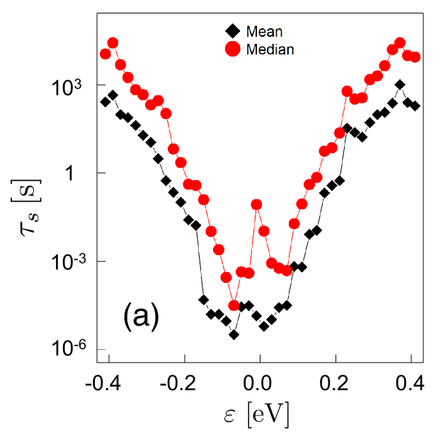
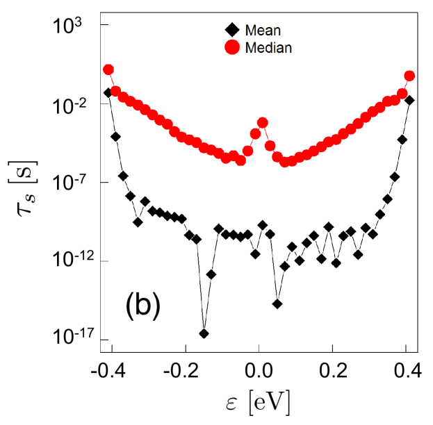
Figure 1: Spin relaxation time as a function of the Fermi energy for hBN (a) and SiO₂ (b) substrates. Black diamonds are mean-generated values while red circles are median-generated.

Figure 1 also shows that $\tau_{s}$ (obtained by the mean value) is relatively low at energies close to the charge neutrality point or low doping and increases by orders of magnitude at large doping values. This behavior is similar for both the mean and median curves, showing that it is not dictated by outliers.

In order to shed some light onto the origin of the behavior seen for $\tau_{s}$ in Fig. 1, we study the coupling matrix elements $t_{\beta 0}$, which is a key element for the calculation of $J_{\beta\beta^{\prime}}$. Figure 2 shows $|t_{\beta 0}|$ for a representative single-disorder realization. The coupling matrix elements $|t_{\beta 0}|$ show strong fluctuations and an exponential average decrease for large $|\varepsilon|$. The coupling magnitudes for hBN, Fig. 2a, are smaller than that for SiO₂, Fig. 2b, which is in agreement with the behavior of $\tau_{s}$ in Fig. 1.

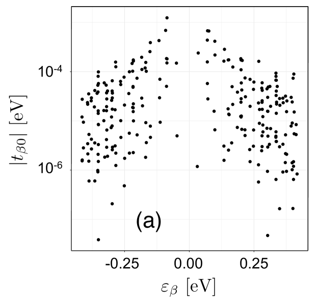
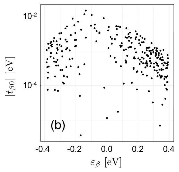
Figure 2: Energy dependence of $|t_{\beta 0}|$ for a single disorder realization of the local potential fluctuations due to hBN (a) and SiO₂ (b) substrates. The magnitude $|t_{\beta 0}|$ is characterized by large fluctuations and an average exponential decay with increasing $|\varepsilon|$.

We note that magnetic textures observed in STM experiments Gonzalez-Herrero et al. (2016); Zhang et al. (2016); Mao et al. (2016) in defective graphene extend up to a radius of about 2 nm around the defect and, hence, are much more localized than the defect-induced state $|0\rangle$ we obtain in our model. This observation motivates us to introduce a cutoff radius $R$ to the localized wave function and study $\tau_{s}$ as a function of $R$.

In Fig. 3 we plot the results obtained when $R\approx 1$ Å, i.e., when the wave function is roughly restricted to the nearest neighbors of the defect and $R\approx 2$ nm, which is the radius determined in experiments Gonzalez-Herrero et al. (2016); Zhang et al. (2016); Mao et al. (2016). Remarkably, Fig. 3 shows that the exponential energy dependence of the hoppings $|t_{\beta 0}|$ vanishes and only a random pattern is left.

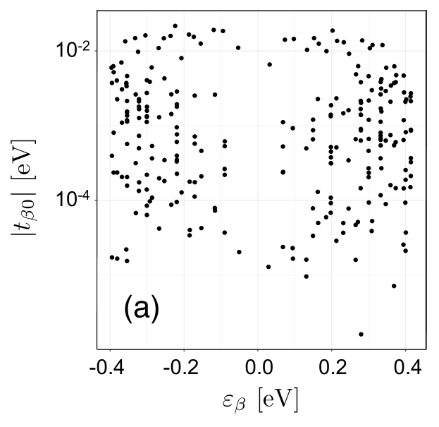
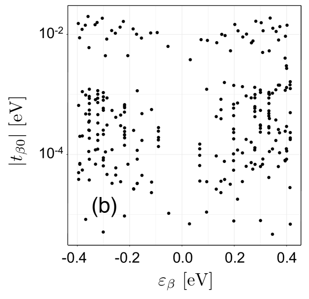
Figure 3: Energy dependence of $|t_{\beta 0}|$ for a single disorder realization of hBN considering the impurity state confined within a radius (a) $R=1$ Å and (b) $R=2$ nm around the defective site. Correlations are quenched and only a random pattern is seen. The same change is obtained for the SiO₂ case (not shown).

The influence of the extension of the quasilocalized state $|0\rangle_{R}$ on $\tau_{s}$ is shown in Fig. 4 for $R=1$ Å  and $R=2$ nm for graphene on SiO₂. The values of $\tau_{s}$ at low doping ($\varepsilon$ close to the Dirac point) is similar to those of the extended midgap state $|0\rangle$, Fig. 1. In contrast, the exponential dependence of $\tau_{s}$ observed for larger values of $|\varepsilon|$ in the $|0\rangle$ case is strongly suppressed when considering $|0\rangle_{R}$-states. This is in line with the above discussion of the coupling matrix $t_{\beta 0}$. We note that the dependence on $R$ is also weak. A comparison between the curves for the mean and median shows that some outliers still push the mean estimates down compared to the median estimates and leads to larger fluctuations. These results are in very good agreement with experimental measurements Balakrishnan et al. (2013); Wojtaszek et al. (2013); McCreary et al. (2012).

For hBN, our simulations (not shown here), when using $\delta W=5.5$ meV, give $\tau_{s}$ values larger (by a factor 10 to 100 times) than those reported in the literature Balakrishnan et al. (2013); McCreary et al. (2012); Wojtaszek et al. (2013); Drogeler et al. (2016). This observation suggests that the effect of outliers is less influent for cleaner samples. However, experiments show that the disorder strength $\delta W$ can increase as one approaches the charge neutrality point Samaddar et al. (2016) and hence a more detailed experimental characterization of the puddles strength is necessary before ruling out the spin relaxation due to magnetic impurities in hBN.

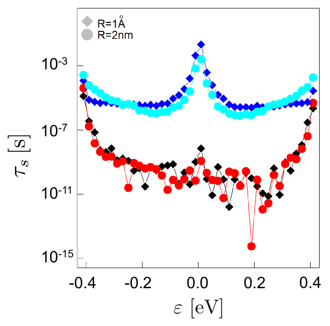
Figure 4: Relaxation times $\tau_{s}$ for graphene on SiO₂ obtained by considering a radial cutoff in the impurity wave functions $|0\rangle_{R}$, for $R=1$ Å (diamonds) and $R=2$ nm (circles). Black- and red-colored symbols denote mean-generated values while blue- and cyan-colored symbols denote median-generated.

The peak structure, such as the median $\tau_{s}$ values for $\varepsilon\approx 0$ in Fig. 4, has been reported in previous theoretical studies Kochan et al. (2014); Soriano et al. (2015); Thomsen et al. (2015). In Refs. Kochan et al., 2014; Soriano et al., 2015, this peak is attributed to an enhanced spin-flip resonant scattering process due the presence of two resonance states, singlet and triplet, with opposite energies close to $\varepsilon=0$, combined with graphene’s vanishing density of states as $\varepsilon\rightarrow 0$. Since our model deals with the magnetic regime of the Anderson model, we interpret such behavior as simply due to the lack of conduction electron states around $\varepsilon=0$. Also, we show that long-ranged disorder does not quench the peak, unless the outliers are present in the system, as seen by comparing the median and mean value estimates for $\tau_{s}$ in Fig. 4.

In Fig. 5, we study the influence of the midgap states energies in the calculation of $\tau_{s}$. As we discussed earlier, in graphene a localized magnetic impurity remains magnetic even when $\varepsilon_{r}>0$ Uchoa et al. (2008) and the presence of such magnetic states have a great impact on the $\tau_{s}$ estimates being responsible for the approximately particle-hole symmetric behavior of $\tau_{s}$ seen in Fig. 5 for the unrestricted curve. The simulations imposing $\varepsilon_{r}<0$ show a huge particle-hole asymmetry, namely, the values of $\tau_{s}$ for $\varepsilon>0$ are orders of magnitude larger than those calculated in the unrestricted case. Such findings show that an unbalance between $\varepsilon_{r}>0$ and $\varepsilon_{r}<0$ states can be the origin of the asymmetric gate voltage dependence of $\tau_{s}$ observed in a recent experiment Drogeler et al. (2016). Such electron-hole asymmetry in spin relaxation rates has also been reported for fluorinated graphene Bundesmann et al. (2015) where the resonance energy lies at $-0.2$ eV, in agreement with our discussion.

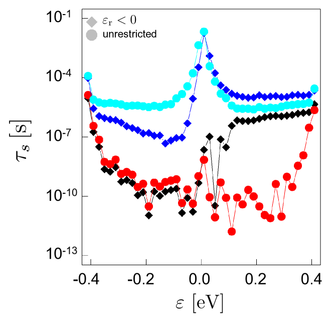
Figure 5: Comparison between $\tau_{s}$ for $\epsilon_{\rm r}<0$ only and the unrestricted ($\epsilon_{\rm r}\lessgtr 0$) case. Black- and red-colored symbols denote mean-generated values while blue- and cyan-colored symbols denote median-generated.

In the simulations shown so far, we have used $U=0.01$eV, a value inferred from experiments Ref. Gonzalez-Herrero et al., 2016; Zhang et al., 2016. However, it is expected that changes in the impurity environment lead to a different screening of the impurity Luican-Mayer et al. (2014), and hence different $U$ values. In Fig. 6 we study the mean value $\tau_{s}$ dependence on $U$. Since Fig. 5 indicates that $\tau_{s}$ is weakly dependent on $R$, we use $|0\rangle_{R}$ with $R=1$ Å.

Figure 6 shows that for $0.01<U<0.1$ eV changing $U$ roughly leads to a rigid shift of the $\tau_{s}$ curves. This range of $U$ values is consistent with what is reported by STM experiments for hydrogenated graphene Gonzalez-Herrero et al. (2016) and graphene with vacancies Zhang et al. (2016). Interestingly, increasing $U$ implies in faster spin relaxation times, showing that screening is an important ingredient in the computation of the spin relaxation, a feature that has not been explored in previous studies Kochan et al. (2014); Soriano et al. (2015); Thomsen et al. (2015); Vierimaa et al. (2017). We also find that the dependence of $\tau_{s}$ on $U$ becomes negligible for $U\gtrsim 1$ eV,

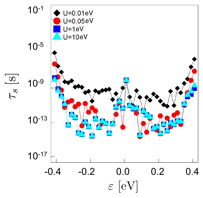
Figure 6: The dependence of $\tau_{s}$ on the charging energy $U$. Mean value estimates obtained for the $|0\rangle_{R}$ impurity state for $R=1$ Å in graphene on a SiO₂ substrate. Data presented for $U=0.01$ eV (diamonds), $U=0.05$ eV (circles), $U=1$ eV (squares), and $U=10$ eV (triangles).

III.2 Adatom

In this section we analyze the spin relaxation occurring due to the magnetism induced by hydrogen adatoms in graphene. In Fig. 7, we plot $\tau_{s}$ as a function of energy for different impurity states $|0\rangle_{R}$, with $R=0$, 1Å, and 2 nm for SiO₂.

The configuration with $R=0$ corresponds to the case where the magnetism is restricted to the hydrogen adatom site. This case has no counterpart in the vacancy-induced magnetism discussed in the previous section. Figure 7a shows that, apart from fluctuations, the mean $\tau_{s}(\varepsilon)$ is approximately the same for the $R=0$, $R=1$ Å, and $R=2$ nm magnetic configurations. On the other hand, a significant departure between the $R=0$ and the remaining configurations is observed in the median $\tau_{s}(\varepsilon)$ curves, see Fig. 7b. For $\varepsilon$ away from the Dirac point the $\tau_{s}(\varepsilon)$ median values for the $|0\rangle_{R=0}$ state are roughly an order of magnitude larger than the $R=1$ Å and $R=2$ nm configurations.

Our results indicate that $\tau_{s}$ is very insensitive to the extent $R$ of the impurity state, which explains why models with different kinds of impurity-states find $\tau_{s}(\varepsilon)$ spin relaxation times in the same range Kochan et al. (2014); Soriano et al. (2015); Thomsen et al. (2015); Vierimaa et al. (2017). Whereas the median $\tau_{s}(\varepsilon)$ in Fig. 7 shows a strong dependence on $R$, the experimentally observed $\tau_{s}(\varepsilon)$ Balakrishnan et al. (2013); Wojtaszek et al. (2013); McCreary et al. (2012) and the $\tau_{s}(\varepsilon)$ obtained by different theoretical models Kochan et al. (2014); Soriano et al. (2015); Thomsen et al. (2015); Vierimaa et al. (2017) is the one dictated by the mean and ruled by the “outliers”, which have same magnitude regardless of the impurity-induced states $R$ for the cases where $R<2$ nm, the one reported experimentally Zhang et al. (2016). Our findings justifies the use of models with very localized impurity states, as in Ref. Kochan et al., 2014 for the $\tau_{s}$ calculation, although the use of such models might become inadequate for the case where the influence of outliers is not relevant.

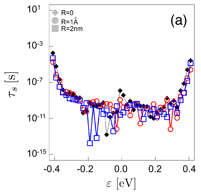
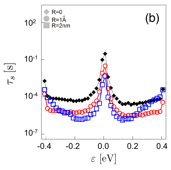
Figure 7: The $\tau_{s}$ dependence on energy of different impurity-induced states for the adatom model: (a) mean and (b) median $\tau_{s}$ values for SiO₂ substrates. The impurity states $|0\rangle_{R}$ considered are $R=0$, $R=1$Å, and $R=2$ nm.

IV Discussion and Conclusions

In this work we studied the problem of spin relaxation due to defect-induced magnetism in graphene. In our approach we developed a microscopic modeling that allows the incorporation of the effect of charge puddles and its interplay with the defect-induced magnetic texture. We showed that the puddles play a key role in the spin relaxation, as it allows for the coupling between the conduction electrons and the impurity-induced state which is responsible for the spin flipping scattering process.

Our microscopic derivation consolidates and improves the previous theoretical approaches Soriano et al. (2015); Kochan et al. (2014); Thomsen et al. (2015); Vierimaa et al. (2017), since the systematic study of the model parameters unraveled how the spin relaxation is influenced by different aspects, such as the quality of the substrate, represented by the disorder parameters, the extent of the magnetic texture, the resonances position, and the charging energy $U$. We stress that the parameters we use in our model are in good agreement with the values reported in the experimental literature.

Figure 8 summarizes our findings, both for vacancy and adatom-induced spin relaxation in graphene. Using experimentally-inferred parameter models, we obtained $\tau_{s}$ as a function of the Fermi energy $\varepsilon$ in the presence of the impurity state $|0\rangle_{R}$, with $R=1$ Å, and found that both spin-relaxation mechanisms show a remarkable agreement. These results are also in agreement with the experiment reported in Ref. McCreary et al., 2012, which observed a similar spin relaxation behavior for graphene with adatoms or vacancies.

These results strongly support the picture that spin relaxation in hydrogenated graphene is dominated by induced magnetism, and not by induced spin-orbit coupling, contradicting the argument presented in Ref. Balakrishnan et al., 2013. This is in agreement with a recent experiment Raes et al. (2016) that found no evidence of a spin-lifetime anisotropy, thus ruling out the spin-orbit coupling as a source of ultrafast spin relaxation. Our findings also falsify the conjecture Thomsen et al. (2015) that discrepancies in $\tau_{s}(\varepsilon)$ calculated by different groups could be due to the defect model choice, namely, adatom Kochan et al. (2014); Thomsen et al. (2015) or vacancy Soriano et al. (2015).

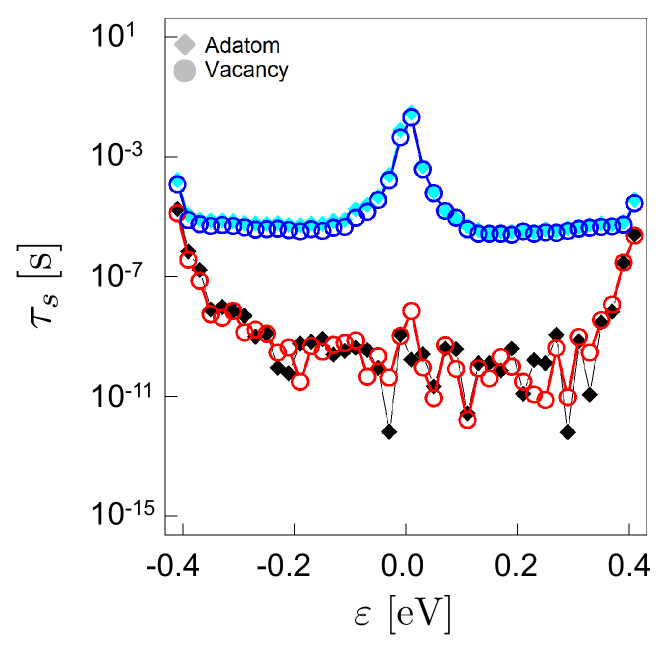
Figure 8: Spin relaxation time $\tau_{s}$ as a function of the Fermi energy: comparison between the vacancy and the adatom models for graphene on SiO₂ and $|0\rangle_{R}$, with $R=1$ Å.

Our study also sheds light onto other controversial issues. One of the main puzzles associated to spin relaxation related to magnetic-induced defects in graphene is whether the spin relaxation is dominated by the Elliot-Yaffet (EY) or the Dyakonov-Perel (DP) mechanism Soriano et al. (2015). Enhancement of $\tau_{s}(\varepsilon)$ after intentional introduction of defects in graphene has been reported in Refs. Wojtaszek et al., 2013; McCreary et al., 2012, suggesting the DP mechanism is responsible for the relaxation process. However, the DP mechanism should be related to random, induced magnetic fields due the impurities. In this regard, experimental results diverge and a conflicting scenario about the random magnetic-induced field interpretation has been questioned Wojtaszek et al. (2013); McCreary et al. (2012).

Here, we propose a new alternative explanation for such a controversy. As has been proposed theoretically Yazyev (2010) and recently confirmed by STM experiments Gonzalez-Herrero et al. (2016), the $\pi$-like magnetism induced by defects in graphene relies on an unbalance between the number of sites in graphene’s sublattices. As a consequence, such magnetism can be turned on/off by placing defects in graphene in a unbalanced/balanced manner Gonzalez-Herrero et al. (2016) among the sublattices.

As we have shown in our study, the main cause of the spin relaxation is the $\pi$-like magnetism and is essentially independent from the source of this magnetism, as can be observed in Fig. 8 for the case of vacancies and hydrogen adatoms. We note that other adatom or molecular species have been proposed to cause a similar $\pi$-like magnetism in graphene, such as methyl Zollner et al. (2016) and fluor Nanda et al. (2012). The fact that different sources may lead to a similar mechanism makes more plausible that $\pi$-like magnetism is present in different experimental scenarios, even when the defects are not intentionally created.

As has been shown in a recent quantum-interference experiment Lara-Avila et al. (2015), localized spinfull scatterers are present in graphene on SiC and are responsible for a fast spin relaxation in such system. Magnetic-induced spin relaxation has also been observed in quantum interference experiments in graphene on SiO₂ Lundeberg et al. (2013). Although a detailed characterization of the source of such magnetic scatterers is still lacking, such similar findings in different scenarios reinforce our arguments.

We speculate that one or some of the species that can induce $\pi-$like magnetism in graphene are present in the samples of Refs. Wojtaszek et al., 2013; McCreary et al., 2012 before the hydrogenation process and some outliers dominate $\tau_{s}(\varepsilon)$ prior to the defect exposition. After the hydrogenation, the magnetic texture due to some of these outliers can be turned off due to the placement of a hydrogen or vacancy in the opposite sublattice with respect to the one that contained the magnetic outlier impurity already in the system. As a result, two spinless scatterers are added, which can reduce the diffusion in the system but cannot flip the conduction electrons spin they scatter. Hence, $\tau_{s}(\varepsilon)$ increases (due to the outlier turn off) and the diffusion coefficient $D$ decreases (due the extra scattering centers after hydrogenation), in agreement with the behavior reported in Ref. Wojtaszek et al., 2013.

This kind of effect seems to be a unique feature of the unusual defect induced $\pi$-like magnetism in graphene, as shown in a recent study Omar et al. (2015) of a graphene spin valve device with cobalt porphyrin (CoPP) molecules. These molecules possess a magnetic moment, which is extrinsic to graphene. In these systems, no enhancement of $\tau_{s}(\varepsilon)$ is observed after the introduction of the magnetic molecules. In fact, the findings in Ref. Omar et al., 2015 enforce the conjecture that outlying magnetic $\pi$-like scatterers rule the spin relaxation process since the effect of the introduction of CoPP on $\tau_{s}(\varepsilon)$ is reported to only be significant in the better quality samples, and unnoticible for the low-quality ones, which are the ones with a higher chance for having $\pi-$like spin scatterers be dominating the relaxation process.

A detailed study of the conditions that lead to the appearance of outliers ruling $\tau_{s}(\varepsilon)$ is necessary to clarify such conjectures and will be addressed in a future work.

Since we show that the energy position of the resonances introduced by defects are essential for the magnitude and symmetry of the $\tau_{s}(\varepsilon)$ curves, our results also allow us to interpret the asymmetric gate-voltage dependence of $\tau_{s}(\varepsilon)$ seen in Ref. Drogeler et al. (2016) as an unbalance between resonances with opposite signs. As different species with different on-site energies $\varepsilon_{0}$ can lead to $\pi$-like magnetism Gmitra et al. (2013); Zollner et al. (2016); Miranda et al. (2016); Nair et al. (2012) and the shift in $\varepsilon_{0}$ is smaller for systems with lower disorder [see Eq. (10)], the asymmetry seen in ultraclean graphene hBN systems can be due to the predominance of resonances of a given sign.

Finally, our findings suggest an interesting opportunity to control $\tau_{s}(\varepsilon)$ and hence build spintronic devices via a functionalization process of graphene with adatoms as the one recently reported for the precise manipulation of hydrogen adatoms on graphene via a STM apparatus Gonzalez-Herrero et al. (2016). By changing the substrate, the defect species giving rise to the induced magnetism, and the relative position among the defects in the graphene lattice, a plethora of possibilities become available for building devices with different spin properties.

Appendix A Numerical details

In this Appendix we provide a detailed description of the numerical analysis used in this work. We focus on two aspects: (i) approximate diagonalization scheme and (ii) histogram binning.

Approximate diagonalization scheme: The computation of $\tau_{s}$, as outlined in Sec. II, requires two steps: First, the diagonalization of $H^{\rm def}$, which gives the $\left\{|\phi\rangle\right\}$ and $|0\rangle$ basis states. Second, a basis change from the $\left\{|\phi\rangle\right\}$ to the $\left\{|\beta\rangle\right\}$ subspace. The latter step requires one to build and diagonalize $H_{PP}$, which is a dense matrix. As a consequence, considering that disorder averaging is necessary, the approach becomes prohibitive already for relative small lattice sizes around $10^{3}$ sites.

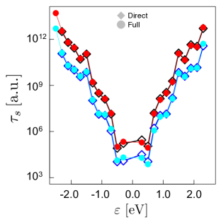
Figure 9: Comparison between the direct (diamonds) and full (circles) diagonalization approaches for a lattice with $N_{\rm tot}=40\times 40$ for $\delta W=0.002t$, corresponding to a hBN substrate. Estimates are obtained using the median (black and red) and mean (blue and cyan).

To access large system sizes, we introduce a subtle change in the approach summarized above. We bypass the basis transformation $\left\{|\phi\rangle\right\}\rightarrow\left\{|\beta\rangle\right\}$ and directly diagonalize $H^{\rm def}+V_{{\rm dis}}$, which involves dealing only with sparse matrices. As a result, for every disorder realization we compute a set of orthogonal extended states $\{|\tilde{\beta}\rangle\}$ and a quasilocalized state $|\tilde{0}\rangle$. We replace the $|\tilde{0}\rangle$ state by $|0\rangle$, the midgap state defined in Eq. (4), and take $\epsilon_{\beta}\rightarrow\epsilon_{\tilde{\beta}}$ and $t_{\beta 0}\rightarrow t_{\tilde{\beta}0}$. Figure 9 shows that the full and the direct diagonalization schemes are in very good agreement, since $\epsilon_{\beta}\approx\epsilon_{\tilde{\beta}}$ and $t_{\beta 0}\approx t_{\tilde{\beta}0}$.

Notice that the approximation scheme also requires two diagonalization steps. However, the diagonalization of $H^{\rm def}$ to obtain $|0\rangle$ is done only once and the diagonalization of $H^{\rm def}+V_{\rm dis}$ involves only sparse matrices, which leads to a huge memory saving and allows for an efficient use of the Lanczos algorithm to obtain the eigenstates $|\tilde{\beta}\rangle$ in a small energy window around $\varepsilon=0$, in accordance with experimental values.

Histogram approach to calculate $\tau_{s}$: The Fermi golden rule, Eq. (25), enforces elastic scattering by a Dirac delta function in energy. In any practical calculation, the latter needs to be smoothen. Our strategy is to use a “histogram approach”: For each disorder realization we construct a histogram of the energies $\varepsilon_{\beta}$. We label the midpoint of each bin of the histogram as $\varepsilon_{i}$. Within each histogram bin we evaluate the spin relaxation time per eigenstate, according to Eq. (33). Averaging $\tau^{m}_{s;\beta}$ inside each interval leads to the $\tau_{s}^{m}(\varepsilon)$, where the energies are given by the set of the histogram midpoints.

The bin size choice is such that it is not large enough to overcome the gap and small enough to reproduce the low energy density of states of graphene. In this paper we take bin widths of $20$ meV.

References

- Han et al. (2014) W. Han, R. K. Kawakami, M. Gmitra, and J. Fabian, Nat. Nano 9, 794 (2014).
- Roche and Valenzuela (2014) S. Roche and S. O. Valenzuela, J. Phys. D: Appl. Phys. 47, 094011 (2014).
- Pesin and MacDonald (2012) D. Pesin and A. H. MacDonald, Nat. Mater. 11, 409 (2012).
- Soriano et al. (2015) D. Soriano, D. V. Tuan, S. M.-M. Dubois, M. Gmitra, A. W. Cummings, D. Kochan, F. Ortmann, J.-C. Charlier, J. Fabian, and S. Roche, 2D Mater. 2, 022002 (2015).
- Fabian et al. (2007) J. Fabian, C. Ertler, A. Matos-abiague, and I. Žutić, Acta Phys. Slovaca 57, 565 (2007).
- Žutić et al. (2004) I. Žutić, J. Fabian, and S. Das Sarma, Rev. Mod. Phys. 76, 323 (2004).
- Tombros et al. (2007) N. Tombros, C. Jozsa, M. Popinciuc, H. T. Jonkman, and B. J. van Wees, Nature 448, 571 (2007).
- Wojtaszek et al. (2013) M. Wojtaszek, I. J. Vera-Marun, T. Maassen, and B. J. van Wees, Phys. Rev. B 87, 081402 (2013).
- Maassen et al. (2013) T. Maassen, J. J. van den Berg, E. H. Huisman, H. Dijkstra, F. Fromm, T. Seyller, and B. J. van Wees, Phys. Rev. Lett. 110, 067209 (2013).
- Omar et al. (2015) S. Omar, M. Gurram, I. J. Vera-Marun, X. Zhang, E. H. Huisman, A. Kaverzin, B. L. Feringa, and B. J. van Wees, Phys. Rev. B 92, 115442 (2015).
- Balakrishnan et al. (2013) J. Balakrishnan, G. Kok Wai Koon, M. Jaiswal, A. Castro Neto, and B. Ozyilmaz, Nat Phys 9, 284 (2013).
- Han and Kawakami (2011) W. Han and R. K. Kawakami, Phys. Rev. Lett. 107, 047207 (2011).
- McCreary et al. (2012) K. M. McCreary, A. G. Swartz, W. Han, J. Fabian, and R. K. Kawakami, Phys. Rev. Lett. 109, 186604 (2012).
- Drogeler et al. (2016) M. Drogeler, C. Franzen, F. Volmer, T. Pohlmann, L. Banszerus, M. Wolter, K. Watanabe, T. Taniguchi, C. Stampfer, and B. Beschoten, Nano Lett. 16, 3533 (2016).
- Ertler et al. (2009) C. Ertler, S. Konschuh, M. Gmitra, and J. Fabian, Phys. Rev. B 80, 041405 (2009).
- Ochoa et al. (2012) H. Ochoa, A. H. Castro Neto, and F. Guinea, Phys. Rev. Lett. 108, 206808 (2012).
- Fedorov et al. (2013) D. V. Fedorov, M. Gradhand, S. Ostanin, I. V. Maznichenko, A. Ernst, J. Fabian, and I. Mertig, Phys. Rev. Lett. 110, 156602 (2013).
- Tuan et al. (2014) D. V. Tuan, F. Ortmann, D. Soriano, S. O. Valenzuela, and S. Roche, Nat. Phys. 10, 857 (2014).
- Bundesmann et al. (2015) J. Bundesmann, D. Kochan, F. Tkatschenko, J. Fabian, and K. Richter, Phys. Rev. B 92, 081403 (2015).
- Huang et al. (2016) C. Huang, Y. D. Chong, and M. A. Cazalilla, Phys. Rev. B 94, 085414 (2016).
- Kochan et al. (2014) D. Kochan, M. Gmitra, and J. Fabian, Phys. Rev. Lett. 112, 116602 (2014).
- Wilhelm et al. (2015) J. Wilhelm, M. Walz, and F. Evers, Phys. Rev. B 92, 014405 (2015).
- Vierimaa et al. (2017) V. Vierimaa, Z. Fan, and A. Harju, Phys. Rev. B 95, 041401 (2017).
- Van Tuan et al. (2016) D. Van Tuan, F. Ortmann, A. W. Cummings, D. Soriano, and S. Roche, Sci. Rep. 6, 21046 (2016).
- Cummings and Roche (2016) A. W. Cummings and S. Roche, Phys. Rev. Lett. 116, 086602 (2016).
- Thomsen et al. (2015) M. R. Thomsen, M. M. Ervasti, A. Harju, and T. G. Pedersen, Phys. Rev. B 92, 195408 (2015).
- Van Tuan and Roche (2016) D. Van Tuan and S. Roche, Phys. Rev. Lett. 116, 106601 (2016).
- Yazyev and Helm (2007) O. V. Yazyev and L. Helm, Phys. Rev. B 75, 125408 (2007).
- Yazyev (2010) O. V. Yazyev, Rep. Prog. Phys. 73, 056501 (2010).
- Miranda et al. (2016) V. G. Miranda, L. G. G. V. Dias da Silva, and C. H. Lewenkopf, Phys. Rev. B 94, 075114 (2016).
- Lieb (1989) E. H. Lieb, Phys. Rev. Lett. 62, 1201 (1989).
- Pereira et al. (2008) V. M. Pereira, J. M. B. Lopes dos Santos, and A. H. Castro Neto, Phys. Rev. B 77, 115109 (2008).
- Inui et al. (1994) M. Inui, S. A. Trugman, and E. Abrahams, Phys. Rev. B 49, 3190 (1994).
- Chang and Haas (2011) Y. C. Chang and S. Haas, Phys. Rev. B 83, 085406 (2011).
- Nanda et al. (2012) B. R. K. Nanda, M. Sherafati, Z. S. Popović, and S. Satpathy, New J. Phys. 14, 83004 (2012).
- Palacios et al. (2008) J. J. Palacios, J. Fernández-Rossier, and L. Brey, Phys. Rev. B 77, 195428 (2008).
- Gonzalez-Herrero et al. (2016) H. Gonzalez-Herrero, J. M. Gomez-Rodriguez, P. Mallet, M. Moaied, J. J. Palacios, C. Salgado, M. M. Ugeda, J.-Y. Veuillen, F. Yndurain, and I. Brihuega, Science 352, 437 (2016).
- Zhang et al. (2016) Y. Zhang, S.-Y. Li, H. Huang, W.-T. Li, J.-B. Qiao, W.-X. Wang, L.-J. Yin, K.-K. Bai, W. Duan, and L. He, Phys. Rev. Lett. 117, 166801 (2016).
- Castro Neto and Guinea (2009) A. H. Castro Neto and F. Guinea, Phys. Rev. Lett. 103, 026804 (2009).
- Gmitra et al. (2013) M. Gmitra, D. Kochan, and J. Fabian, Phys. Rev. Lett. 110, 246602 (2013).
- Soriano et al. (2011) D. Soriano, N. Leconte, P. Ordejón, J.-C. Charlier, J.-J. Palacios, and S. Roche, Phys. Rev. Lett. 107, 016602 (2011).
- Wehling et al. (2009) T. O. Wehling, M. I. Katsnelson, and A. I. Lichtenstein, Phys. Rev. B 80, 085428 (2009).
- Robinson et al. (2008) J. P. Robinson, H. Schomerus, L. Oroszlány, and V. I. Fal’ko, Phys. Rev. Lett. 101, 196803 (2008).
- Miranda et al. (2014) V. G. Miranda, L. G. G. V. Dias da Silva, and C. H. Lewenkopf, Phys. Rev. B 90, 201101 (2014).
- Flach et al. (2014) S. Flach, D. Leykam, J. D. Bodyfelt, P. Matthies, and A. S. Desyatnikov, EPL (Europhysics Letters) 105, 30001 (2014).
- Martin et al. (2008) J. Martin, N. Akerman, G. Ulbricht, T. Lohmann, J. H. Smet, K. von Klitzing, and A. Yacoby, Nat. Phys. 4, 144 (2008).
- Xue et al. (2011) J. Xue, J. Sanchez-Yamagishi, D. Bulmash, P. Jacquod, A. Deshpande, K. Watanabe, T. Taniguchi, and B. J. Jarillo-Herrero, Pablo LeRoy, Nat. Mater. 10, 282 (2011).
- Zhang et al. (2009) Y. Zhang, V. W. Brar, C. Girit, A. Zettl, and M. F. Crommie, Nat. Phys. 5, 722 (2009).
- Mucciolo and Lewenkopf (2010) E. R. Mucciolo and C. H. Lewenkopf, J. Phys.: Condens. Matter 22, 273201 (2010).
- Adam et al. (2011) S. Adam, S. Jung, N. N. Klimov, N. B. Zhitenev, J. A. Stroscio, and M. D. Stiles, Phys. Rev. B 84, 235421 (2011).
- Burgos et al. (2015) R. Burgos, J. Warnes, L. R. F. Lima, and C. Lewenkopf, Phys. Rev. B 91, 115403 (2015).
- Padmanabhan and Nanda (2016) H. Padmanabhan and B. R. K. Nanda, Phys. Rev. B 93, 165403 (2016).
- Palacios and Ynduráin (2012) J. J. Palacios and F. Ynduráin, Phys. Rev. B 85, 245443 (2012).
- Samaddar et al. (2016) S. Samaddar, I. Yudhistira, S. Adam, H. Courtois, and C. B. Winkelmann, Phys. Rev. Lett. 116, 126804 (2016).
- Anderson (1961) P. W. Anderson, Phys. Rev. 124, 41 (1961).
- Hewson (1993) A. C. Hewson, The Kondo Problem to Heavy Fermions, 1st ed. (Cambridge University Press, Cambridge, 1993).
- Schrieffer and Wolff (1966) J. R. Schrieffer and P. A. Wolff, Phys. Rev. 149, 491 (1966).
- Note (1) Strictly speaking this is not a perturbative approach since high-order terms contribute to the corrections due to . The approach aims to isolate these interaction terms by applying the canonical transformation and eliminating to first order.
- Uchoa et al. (2008) B. Uchoa, V. N. Kotov, N. M. R. Peres, and A. H. Castro Neto, Phys. Rev. Lett. 101, 026805 (2008).
- Phillips (2012) P. Phillips, Advanced Solid State Physics, 2nd ed. (Cambridge University Press, Cambridge, 2012).
- Kondo (1964) J. Kondo, Progress of Theoretical Physics 32, 37 (1964).
- Zunger and Englman (1978) A. Zunger and R. Englman, Phys. Rev. B 17, 642 (1978).
- Nair et al. (2012) R. R. Nair, M. Sepioni, I.-L. Tsai, O. Lehtinen, J. Keinonen, A. V. Krasheninnikov, T. Thomson, A. K. Geim, and I. V. Grigorieva, Nat. Phys. 8, 199 (2012).
- Just et al. (2014) S. Just, S. Zimmermann, V. Kataev, B. Büchner, M. Pratzer, and M. Morgenstern, Phys. Rev. B 90, 125449 (2014).
- Mao et al. (2016) J. Mao, Y. Jiang, D. Moldovan, G. Li, K. Watanabe, T. Tanigushi, M. R. Masir, F. M. Peeters, and E. Y. Andrei, Nat. Phys. 22, 1745 (2016).
- Note (2) For the sites outside a radius around the defect position, we set the value of the -state amplitudes to zero. The amplitudes of the remaining sites are reweighed such that .
- Luican-Mayer et al. (2014) A. Luican-Mayer, M. Kharitonov, G. Li, C.-P. Lu, I. Skachko, A.-M. B. Gonçalves, K. Watanabe, T. Taniguchi, and E. Y. Andrei, Phys. Rev. Lett. 112, 036804 (2014).
- Raes et al. (2016) B. Raes, J. E. Scheerder, M. V. Costache, F. Bonell, J. F. Sierra, J. Cuppens, J. Van de Vondel, and S. O. Valenzuela, Nat. Commun. 7, 11444 (2016).
- Zollner et al. (2016) K. Zollner, T. Frank, S. Irmer, M. Gmitra, D. Kochan, and J. Fabian, Phys. Rev. B 93, 045423 (2016).
- Lara-Avila et al. (2015) S. Lara-Avila, S. Kubatkin, O. Kashuba, J. A. Folk, S. Lüscher, R. Yakimova, T. J. B. M. Janssen, A. Tzalenchuk, and V. Fal’ko, Phys. Rev. Lett. 115, 106602 (2015).
- Lundeberg et al. (2013) M. B. Lundeberg, R. Yang, J. Renard, and J. A. Folk, Phys. Rev. Lett. 110, 156601 (2013).
- Note (3) In the direct diagonalization, we model vacancies by adding an on-site energy . The result is equivalent to that obtained using Eq. (1\@@italiccorr) and the full diagonalization scheme, but is more practical for a Lanczos diagonanization.