Statistical characterization of discrete conservative systems:
The web map

Abstract

We numerically study the two-dimensional, area preserving, web map. When the map is governed by ergodic behavior, it is, as expected, correctly described by Boltzmann-Gibbs statistics, based on the additive entropic functional $S_{BG}[p(x)]=-k\int dx\,p(x)\ln p(x)$. In contrast, possible ergodicity breakdown and transitory sticky dynamical behavior drag the map into the realm of generalized $q$-statistics, based on the nonadditive entropic functional $S_{q}[p(x)]=k\frac{1-\int dx\,[p(x)]^{q}}{q-1}$ ($q\in{\cal R};S_{1}=S_{BG}$). We statistically describe the system (probability distribution of the sum of successive iterates, sensitivity to the initial condition, and entropy production per unit time) for typical values of the parameter that controls the ergodicity of the map. For small (large) values of the external parameter $K$, we observe $q$-Gaussian distributions with $q=1.935\dots$ (Gaussian distributions), like for the standard map. In contrast, for intermediate values of $K$, we observe a different scenario, due to the fractal structure of the trajectories embedded in the chaotic sea. Long-standing non-Gaussian distributions are characterized in terms of the kurtosis and the box-counting dimension of chaotic sea.

I Introduction

As well–known, invariant closed curves of area–preserving maps present complete barriers to orbits evolving inside resonance islands in the two–dimensional phase space. Outside these regions, there exist families of smaller islands and invariant Cantor sets, to which chaotic orbits are observed to “stick” for very long times. Thus, at the boundaries of these islands, an “edge of chaos” develops with vanishing or very small Lyapunov exponents, where trajectories yield quasi-stationary states (QSS) that are often very long–lived. Such phenomena have been thoroughly studied to date in terms of a number of dynamical mechanisms responsible for chaotic transport in area–preserving maps and low–dimensional Hamiltonian systems MacKay ; Wiggins .

In such a weakly chaotic regime, chaotic orbits ergodically wander through a subset of the energy surface without ever covering it completely, and “islands of stability” are associated with stable periodic orbits that are caused by invariant curves encircling stable periodic points that exclude the surrounding chaotic trajectory. There are also many island chains that correspond to orbits of different period and a hierarchy of stable points with island chains surrounding island chains ad infinitum. This hierarchical organization causes the surrounding chaotic orbit to have structure at all scales.

A distinctive feature of all fractals is the dependence of the apparent size on the scale of resolution. In this line of approach, Umberger and Farmer characterize chaotic orbits in a two dimensional conservative system as fat fractals that have positive Lebesgue measure but their apparent size depends on the scale of resolution Umberger85 ; Farmer85 . Of course, an orbit is composed of a countable set of points and has no area, but when we refer to the “area of an orbit” we actually mean the Lebesgue measure of the closure of the orbit. Consequently, we can characterize chaotic orbits of a map as fractals if the apparent area occupied by the orbit depends on the resolution used to measure it. However, it is convenient to distinguish the “fat” fractals from “thin” (not fat) fractals of zero Lebesgue measure, such as the strange attractors that appear in dissipative dynamics Cantorlike . In fact, the existence of disjoint invariant regions with a different degree of stochasticity on the same constant energy surface has been investigated by Pettini and Vulpiani in nonlinear hamiltonian systems, and their results do suggest fractal dimensions of the subspaces spanned by the trajectories Pettini84 .

On the other hand, Benettin et al. have investigated the dimensionality of one finite-time trajectory near the unstable manifold of a family of two-dimensional perturbed integrable area preserving maps. They conclude that a finite-time trajectory will necessarily exhibit an apparent fractal dimension, which will be the effective one to all practical purposes: in order to find an effective dimension $d_{f}=2$, one has to look at sufficiently small scales that decrease exponentially fast with the inverse of the parameter of the map Benettin86 .

In this work, we shall consider a particular two-dimensional area-preserving map whose sticky behavior appears to play a significative role in the dynamics, namely, the web map Zaslavskii, (2005). The previous considerations make the complexity of this map susceptible to be studied in the context of generalized $q$-statistics Tsallis ; Tsallis2010 . According to this approach, based on the nonadditive entropy $S_{q}$, whose formulation was inspired in the geometry of multifractals, the probability density functions (pdfs) that optimize $S_{q}$ — under appropriate constraints — are $q^{\prime}$-Gaussian distributions that represent metastable states or QSS of the dynamics. Generalized $q$-statistics manages to characterize meta-stable or stationary states by a triplet of $q$-values, i.e., the $q$-triplet $(q_{sens},q_{rel},q_{stat})$, where sens stands for sensitivity, rel stands for relaxation and stat stands for stationary, whose values collapse to unity when ergodicity is attained (i.e., $q_{sens}=q_{rel}=q_{stat}=1$). In fact, in the case of ergodicity, the Boltzmann-Gibbs entropy is the proper one ($q_{sens}=1$), and Gaussian distributions are observed ($q_{stat}=1$).

In this scenario, we will analyze the dependence of the apparent size on the scale of resolution — the capacity dimension — of the subspace spanned by a set of finite-time trajectories embedded inside the chaotic sea of the web map. This is to reveal, for some paradigmatic values of the parameter of the map, the relation between a fractal dimension of the subspaces spanned by the trajectories embedded inside the chaotic map and their respective pdfs. We will also analyze other parameters that characterize the nonextensivity of the map.

The paper is organized as follows. In Section II we present the area–preserving web map, describing the role of the parameter of the map in the process of ergodicity breakdown and the appearance of QSS. In Section III we analyze the probability distribution of the sum of the iterates of the map, and we exhibit that the fractal dimension of the trajectories embedded inside the apparently chaotic sea — even in the limit of an infinite number of iterations — appears to be a sufficient condition for the convergence to non-Gaussian distributions. In Section IV we analyze non-extensive indices related to the sensitivity to the initial conditions and the entropy production per unit time. Our main conclusions are drawn in Section Conclusions.

II Ergodicity breakdown

The web map is defined as:

$$\begin{array}[]{l}u_{i+1}=v_{i}\\ v_{i+1}=-u_{i}-K\sin(v_{i})\end{array}$$ (1)

where both $u_{n}$ and $v_{n}$ are taken as modulo $2\pi$, and $K$ is the parameter that controls the ergodicity of the map. When $K=0$, the system is integrable and all orbits are $T=4$-periodic. Increasing $K$, invariant orbits that correspond to periodic motion disappear, and stable elliptic periodic points, unstable hyperbolic periodic points and chaotic orbits, appear in their wake. Tuning up the value of $K$, the phase portraits exhibit a clear evolution from a predominance of stability islands all over the phase space (e.g., $K=0.1$) to the flood of a whole chaotic sea that occupies the whole square (e.g.. $K=5.0$). The phase portraits of intermediate cases (e.g., $K=3$, $K=3.5$, $K=3.7$, $K=3.8$, $K=4.5$…) show the stability islands and the chaotic sea coexisting on the full phase space of the map.

For fixed values of $K$, and using Benettin algorithm Benettin, (1980), we calculate the Largest Lyapunov Exponent (LLE) for each initial condition separately — or, alternatively, the Smaller Alignment Index (SALI)— to characterize the orbits and the possible existence of QSS Skokos . In fact, the finite-time contributions coming from the initial conditions of stability islands differ considerably from the ones coming from the strongly chaotic sea. Fig. 1 shows, for a representative value of the map parameter that induces the coexistence of stability islands and chaotic sea, i.e., $K=3.5$, the large but finite-time LLEs that have been obtained for a huge random set of initial conditions all over the phase space. The cumulative distribution of the relative number of initial conditions, as a function of the finite-time LLE threshold, presents an abrupt increase and suggests that we must take into account only two sets of trajectories in the statistics: the strongly chaotic trajectories embedded in a chaotic sea whose LLE $\gg 0$, and the weakly chaotic trajectories whose LLE $\simeq 0$. If we compare this scenario with that one found in the standard map Tirnakli, (2016), an analogous statistical behavior would be expected and, consequently, the coexistence of two different regimes would induce a linear superposition of their respective Gaussian and $q$-Gaussian probability distribution functions. But it is not so, as we will show in Section III.

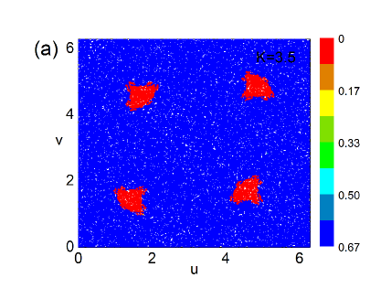
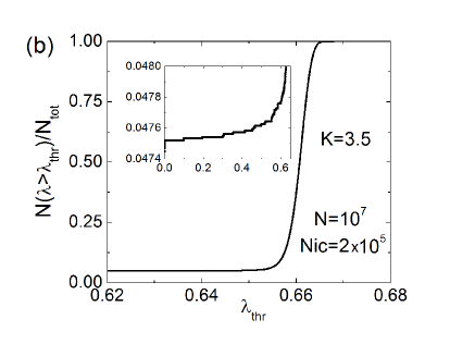
Figure 1: (Color online) (a) Finite-time largest Lyapunov exponent (LLE) of $2\times 10^{5}$ randomly chosen initial conditions of the $K=3.5$ web map, for $10^{7}$ iterations. The Lyapunov spectrum presents largely positive LLE where the phase space is dominated by a chaotic sea, and nearly vanishing LLE in four regions where stability islands dominate the dynamical behavior. (b) Cumulative distribution of the relative number of initial conditions, as a function of a finite-time LLE threshold, $\lambda_{thr}$.

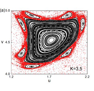
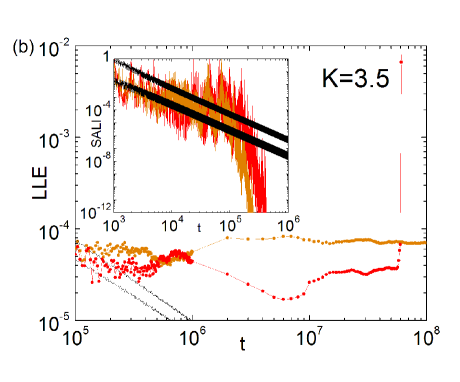
Figure 2: (Color online) (a) A zoom of the phase space of the web map for $K=3.5$, that shows sticky behavior (red trajectories) around quasiperiodic islands (black trajectories). (b) Finite-time LLE and SALI evolution of two quasiperiodic orbits (black), and two strongly chaotic orbits with sticky behavior: one of them (red) escapes after $6\times 10^{7}$ iterations, and the other one (orange) does not escape before $10^{8}$ iterations.

On the other hand, it seems that for some values of the external parameter of the web map — and, in particular, for $K=3.5$ — the sticky effect of strongly chaotic trajectories appears to be statistically much more significant than in the standard map. Fig. 2 exemplifies trajectories with extremely small finite-time LLE that suddenly escape from sticky regions to larger finite-time LLE at larger times. The inverse phenomenon also occurs, as trajectories initially embedded in a strongly chaotic sea (LLE $\gg 0$) can be trapped around the islands (LLE $\sim 0$), after an arbitrarily large time evolution.

Let us now show how ergodicity breakdown and the described transitory sticky dynamical behavior drag the map into the realm of a generalized statistics.

III Stationary and quasistationary distributions

It is well known, through the central limit theorem, that in case of trajectories which are essentially ergodic and mixing, Gaussians are ultimately observed as the probability density distributions of the sums of the iterates of the map. In such cases, the LLE is bounded away from zero. On the contrary, in the case of vanishing LLE, it has been observed that the re-scaled sums are not Gaussians but can instead appear to approach $q$-Gaussian limit distributions. This is in fact the case of the standard map Tirnakli, (2016); Ruiz, (2017) and, for some $K$ values, it is also the case of the web map. But we have also found a third unexpected scenario, for a kind of trajectories embedded inside the chaotic sea — whose LLE is consequently bounded away from zero —, that specially distinguishes the statistical behavior of the web map from that of the standard map. Let us now describe in detail these three distinct scenarios.

In the spirit of the Central Limit Theorem, let us define the variable

$$y=\sum_{i=1}^{N}\left(u_{i}-\langle\,u\,\rangle\right)$$ (2)

where $\langle\,\cdots\rangle$ implies averaging over a large number of iterations $N$ and a large number of randomly chosen initial conditions $M$, i.e., $\langle u\rangle=\frac{1}{M}\frac{1}{N}\sum_{j=1}^{M}\sum_{i=1}^{N}u_{i}^{(j)}$. It was previously shown, for arbitrary values of the parameter $K$ of the standard map Tirnakli, (2016); Ruiz, (2017), that the probability distribution of these sums (Eq. (2)) can be modeled as

$$P_{q}(y;\mu_{q},\sigma_{q})=A_{q}\sqrt{B_{q}}\left[1-(1-q)B_{q}(y-\mu_{q})^{2}\right]^{\frac{1}{1-q}},$$ (3)

that represents the probability density for the initial conditions inside the vanishing Lyapunov region ($q\neq 1$), where $\mu_{q}$ is the $q$-mean value, $\sigma_{q}$ is the $q$-variance, $A_{q}$ is the normalization factor and $B_{q}$ is a parameter which characterizes the width of the distribution prato-tsallis-1999 :

$$A_{q}=\left\{\begin{array}[]{lc}\displaystyle\frac{\Gamma\left[\frac{5-3q}{2(1-q)}\right]}{\Gamma\left[\frac{2-q}{1-q}\right]}\sqrt{\frac{1-q}{\pi}},&q<1\\ \displaystyle\frac{1}{\sqrt{\pi}},&q=1\\ \displaystyle\frac{\Gamma\left[\frac{1}{q-1}\right]}{\Gamma\left[\frac{3-q}{2(q-1)}\right]}\sqrt{\frac{q-1}{\pi}},&1<q<3\end{array}\right.$$ (4)

$$B_{q}=[(3-q)\sigma_{q}^{2}]^{-1}.$$ (5)

The $q$-mean value and $q$-variance are defined by (see prato-tsallis-1999 for the continuous version):

$$\mu_{q}=\frac{\sum_{i=1}^{N}y_{i}[P_{q}(y_{i})]^{q}}{\sum_{i=1}^{N}[P_{q}(y_{i})]^{q}},$$ (6)

$$\sigma_{q}^{2}=\frac{\sum_{i=1}^{N}y_{i}^{2}[P_{q}(y_{i})]^{q}}{\sum_{i=1}^{N}[P_{q}(y_{i})]^{q}},$$ (7)

though we have considered these variables as fitting parameters.

The $q\to 1$ limit recovers the Gaussian distribution $P_{1}(y;\mu_{1},\sigma_{1})=\frac{1}{\sigma_{1}\sqrt{2\pi}}\exp\left[-\frac{1}{2}\left(\frac{y-\mu_{1}}{\sigma_{1}}\right)^{2}\right]$ and, in fact, Fig. 3 shows that, when the trajectories of the web map are essentially ergodic and mixing (LLE is bounded away from zero and a chaotic sea involves the whole phase portrait, e.g., $K=5$), the limit probability distribution of Eq. (2) neatly approaches a Gaussian even for a relatively small number of iterations $N$.

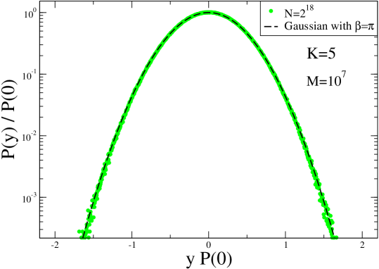
Figure 3: (Color online) The probability distribution function of the sum of the iterates of $K=5$ web map (green dots) neatly fits a Gaussian (dashed line), $P(y)=P(0)e^{-\beta y^{2}}$ where $\beta=3.14$. $N$ and $M$ are the number of iterates and initial conditions, respectively.

On the contrary, when the phase space portrait of the web map is dominated by the stability islands, the probability distribution of Eq. (2) converges to a $q$-Gaussian with $q\simeq 1.935$, as shown in Fig. 4. This convergence has also been observed for values of the map parameter sufficiently close to $K=0$. The persistence of the value $q_{stat}=1.935$ for both the standard and the web maps, when space portrait maps are dominated by stability islands, constitutes an intriguing result.

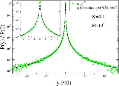
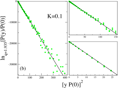
Figure 4: (Color online) (a) $K=0.1$ probability distribution function $P(y)$ (green dots) demonstrates to fit a $q$-Gaussian (dashed line), i.e., $P(y)=P(0)e_{q}^{-\beta y^{2}}$, where $q=1.935$ and $\beta=92$. $N=2^{23}$ and $M=10^{7}$ are the number of iterates and initial conditions, respectively. (b) $q$-logarithmic representation of the same distribution is given for the tail, intermediate and central regions.

On the other hand, intermediate values of $K$, where both chaotic sea and stability islands coexist, appear to confirm that the probability distribution all over the whole phase space of the map is well-fitted by a superposition of a $(q=1.395)$-Gaussian and another distribution. But this case is much more intricate than that of the standard map, and hereinafter we will restrict our analysis to the distributions of trajectories embedded inside the chaotic sea, where we have obtained some astonishing results.

Actually, an unexpected result is that, for particular map parameter values, the probability distribution of the finite trajectories embedded inside the chaotic sea appear to be well far away from a Gaussian even for extremely long iteration times. For relatively large number of iterations ($N\sim 2^{22}$), the probability distribution appears to be well fitted by a $q$-Gaussian but, for even larger iterations, the central part appears to evolve in an extremely slowly rhythm towards a Gaussian, as shown in Fig. 5, but non-Gaussian tails do persist.

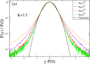
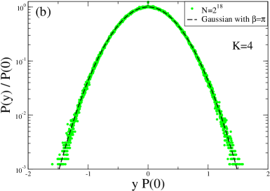
Figure 5: (Color online) (a) Probability distribution function for the iterates of $K=3.5$ web map for various $N$ values. The number of iterations is $M=10^{7}$ all taken from the chaotic sea. (b) The same for $K=4$.

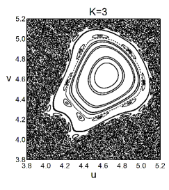
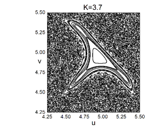
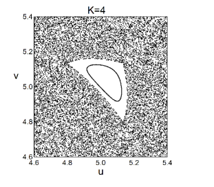
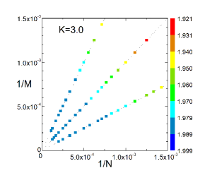
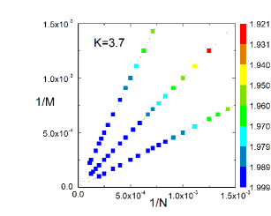
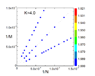
Figure 6: (Color online) Above: Details of the phase portraits of the web map, for three representative values of the map parameter, $K$. Below: Color maps of the box counting dimension of $M$ finite time trajectories embedded inside their respective chaotic sea. $N$ is the number of iterations; the $M$ initial conditions have been randomly chosen all over the band $[2.7,3.8]\times[0,2\pi]$.

We have observed that the values of $K$ where we detect such a behavior appear to be related to the existence in the phase space of a hierarchical organization of island chains of stability that make the surrounding chaotic orbit to have structure at all scales, as we previously pointed out. Consequently, the chaotic trajectories can be characterized as (fat) fractals, and their fractal dimension appears to be $d_{f}<2$. Fig. 6 shows, for some representative map parameter values, the color maps of the box-counting dimension of finite sets (i.e. $M<\infty$) and finite-time trajectories (i.e. $N<\infty$) embedded inside the chaotic sea, together with a detail of their respective phase portraits. The box-counting fractal dimension has been calculated through a Matlab implementation of the Hou algorithm Souza2011 ; Hou76 that optimizes memory storage and significantly reduces time requirements with respect to other box-counting calculation procedures.

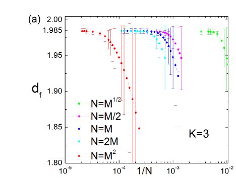
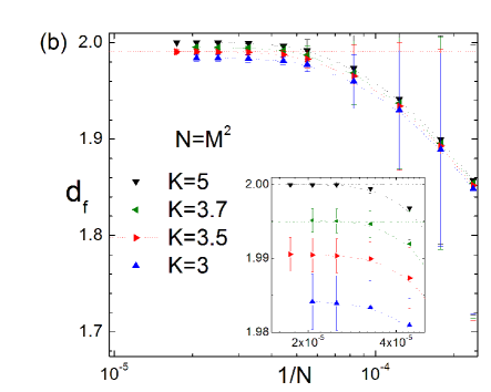
Figure 7: (Color online) (a) Box counting dimension of the phase portrait calculated through the first $N$ iterates of $M$ trajectories in the $K=3$ web map. The initial conditions have been randomly chosen inside the band $[2.7,3.8]\times[0,2\pi]$ and, consequently, the trajectories are embedded in the chaotic sea. In all cases, the $N\to\infty$ limit appears to be $d_{f}=1.985\pm 0.004<2$. (b) The same for some representative values of $K$, and $N=M^{2}$.

The $N\to\infty$ limit probability distributions were expected to be Gaussians. With the aim of characterizing the convergence, we have analyzed the $N\to\infty$ limit of the fractal dimension, as $N\to\infty$ and $M\to\infty$, through different paths over the $(N,M)$ space. Fig. 7 (a) demonstrates, for $K=3$ that, no matter the path to be chosen, the limit box-counting dimension is $d_{f}=1.985\pm 0.004<2$. Fig. 7 (b) shows that an analogous behavior has been found for other values of $K$ ($K=3.5$, $K=3.7$, …) that are associated to slow convergence behavior of the kind shown in Fig. 5 (a). On the contrary, in the case of strongly chaotic phase space ($K=5$) or fast convergence to Gaussian distribution ($K=3.8$ and $K=4$), the $N\to\infty$ box-counting dimension is $d_{f}=2$.

Let us now estimate the kurtosis of the $N\to\infty$ limit pdfs, by calculating the kurtosis of the finite $N$ pdfs, $\kappa$. We will make use of the expression:

$$\kappa=\frac{1}{\sigma^{4}}\left[\frac{1}{M}\sum_{i=1}^{M}(y_{i}-\mu)^{4}\right]$$ (8)

where $y_{i}$ ($i=1,\dots,M$) are the sums of the $N$ iterates in Eq. (2), $\mu$ is the arithmetical average of the sums, and $\sigma$ is the variance. Fig. 8 shows, for some representative values of $K$ that drive to a fractal dimension of the chaotic sea ($d_{f}<2$), that the $N\to\infty$ limit distribution does not in fact appear to converge to a Gaussian, i.e., $\lim_{N\to\infty}\kappa\neq 3$. On the contrary, the values of $K$ that drive to a chaotic sea with $d_{f}=2$, verify $\lim_{N\to\infty}\kappa=3$. Table 1 shows, for typical values of $K$, the estimated ($N\to\infty$) limit value of the kurtosis of the limit pdf, and the estimated values of ($N\to\infty$) limit of fractal dimension in a set of ($M\to\infty$) trajectories. We conclude that a non trivial dependence between $\kappa$ and $d_{f}$ exists. Indeed the fat fractal dimension embedded inside the chaotic sea converges slowly towards some generalized distributions whose long tails preclude a Gaussian characterization.

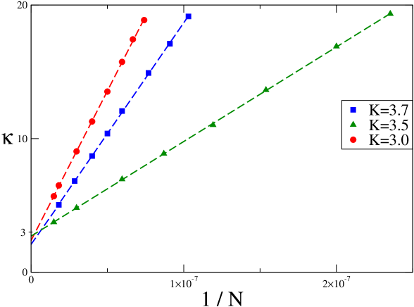
Figure 8: (Color online) Kurtosis of the probability distribution of the sums of iterates of finite-time trajectories that are embedded inside the chaotic sea, for some representative values of the parameter of the map that exhibit a fractal dimension of the chaotic sea $d_{f}<2$. The asymptotic values of the kurtosis are calculated as $\kappa=2.37\pm 0.06$ for $K=3.$, $\kappa=2.70\pm 0.04$ for $K=3.5$ and $\kappa=2.08\pm 0.05$ for $K=3.7$ from the figure. Regression coefficients are about $0.9999$. Observe that the kurtosis does not appear to converge to the characteristic value of a Gaussian, namely $\kappa_{G}=3$. Consequently, we infer that the $N\to\infty$ limit pdf is not a Gaussian.

$K$	$\kappa$	$d_{f}$
$3$	$2.37\pm 0.06$	$1.9846\pm 0.0034$
$3.5$	$2.70\pm 0.04$	$1.9909\pm 0.0020$
$3.7$	$2.08\pm 0.05$	$1.9963\pm 0.0014$
$3.8$	$3$	$2$
$4$	$3$	$1.9989\pm 0.0004$
$5$	$3$	$2$

Table 1: Estimated ($N\to\infty$) limit value of the kurtosis of the limit pdf, and the estimated values of ($N\to\infty$) limit of fractal dimension in a set of ($M\to\infty$) trajectories of typical values of the web map parameter.

IV $q$-statistical indices

The previous section deals with the stationary and quasi stationary characterization of the web map. As we pointed out, in some cases, the finite $N$ probability distribution functions can be properly fitted with a $q$-Gaussian that is characterized by a $q_{stat}$ index. Let us now make a review of other new results related to other $q$-statistical indices, that have been obtained for the web map, and are consistent with the results that were obtained in the standard map Ruiz, (2017).

For many complex systems, the sensitivity to initial conditions, $\xi(t)$ is described by a generalized function, $e_{q}(x)=[1+(1-q)x]^{\frac{1}{1-q}}$ (with $e_{1}(x)=\exp(x)$), referred to as $q$–exponential Plastino, (1997). More precisely,

$$\small{\xi(t)\equiv\lim_{\|{\bf\Delta x}(0)\|\to{\bf 0}}\frac{\|{\bf\Delta x}(t)\|}{\|{\bf\Delta x}(0)\|}=\left[1+(1-q_{sen})\lambda_{q_{sen}}t\right]^{\frac{1}{1-q_{sen}}}\equiv e_{q_{sen}}^{\lambda_{q_{sen}}t}},$$ (9)

${\bf\Delta x}(t)$ being the temporal dependence of the discrepancy between two very close initial conditions at time $t$, where $q_{sen}$ and $\lambda_{q_{sen}}$ (generalized Lyapunov coefficient) are parameters. When ergodic behavior dominates over the whole phase space, Eq. (9) recovers the standard exponential dependence $\xi(t)=e^{\lambda t}$ ($q_{sen}=1$ implies $\lambda_{q_{sen}}\to\lambda\equiv\lambda_{1}$, where $\lambda$ denotes the standard Lyapunov exponent).

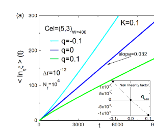
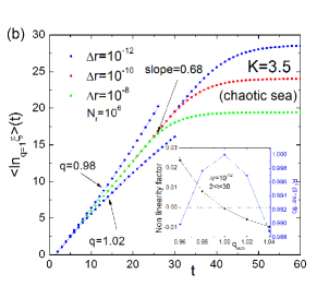
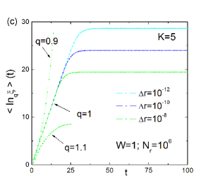
Figure 9: (Color online) Average of the $q$-logarithm of the sensitivity to initial conditions over $N_{r}$ realizations for (a) the $K=0.1$ web map dominated by the regular islands, (b) the chaotic sea of the $K=3.5$ web map, and (c) the $K=5$ web map dominated by the chaotic sea. $\Delta r\equiv{\bf\Delta x}(0)$ is the distance between two initial conditions that have been randomly chosen within a particular cell of the $W$-partitioned phase portrait (see text). Insets demonstrate that (a) $q_{sen}=0$ and $\lambda_{0}=0.032$ inside the $(5^{th},3^{th})$ cell of $W=20\times 20$ equally partitioned $K=0.1$ phase space, and (b) $q_{sen}=1$ and $\lambda_{1}=0.68$ inside the central cell of the $W=3\times 3$ equally partitioned phase space. (c) The $K=5$ web map satisfies $q_{sen}=1$ and $\lambda_{1}=0.96$.

This description is verified for both strongly and weakly chaotic regimes. Fig. 9 shows, for different values of $K$ parameter and different values of $q$, the average of $\ln_{q}\xi(t)$ (where $\ln_{q}x\equiv(x^{1-q}-1)/(1-q)$ is the inverse function of the $q$-exponential, and $\ln_{1}x=\ln x$) over $N_{r}$ realizations. Each realization starts with a randomly chosen pair of very close initial conditions, localized inside a particular cell of the $W$ equally partitioned phase space. We considered decreasing initial discrepancies in Eq. (9) (see Fig. 9 (b-c)), so as to obtain a well defined behavior for increasingly long times, and verify a nontrivial property Ananos, (2004), namely that a special value of $q$ exists, noted $q^{av}_{sen}$ (where $av$ stands for average), which yields a linear dependence of $\langle\ln_{q}\xi\rangle$ with time. In other words, we verify $\langle\ln_{q}\xi(t)\rangle\approx\lambda_{q_{sen}^{av}}t$, where the linear coefficient $\lambda_{q_{sen}^{av}}$ is a $q$-generalized Lyapunov coefficient. When stability islands dominate the phase space ($K=0.1$), Fig. 9 (a) exhibits that $q_{sen}^{av}=0$, and the generalized Lyapunov exponent $\lambda_{q_{sen}^{av}}=0.032\pm 0.001$ (time steps)^-1 characterizes the local sensitivity to initial conditions. In the chaotic sea, e.g., Fig. 9 (b) for the trajectories embedded inside the chaotic sea of the $K=3.5$ map, and Fig. 9 (c) for the strongly chaotic $K=5$ map, where an exponential sensitivity to initial conditions is verified as $q_{sen}^{av}=1$, and the slope of intermediate regimes demonstrate to be $\lambda_{q_{sen}^{av}=1}=0.68\pm 0.01$ (time steps)^-1 and $\lambda_{q_{sen}^{av}=1}=0.96\pm 0.01$ (time steps)^-1, respectively. The proper $q$ indices are obtained by fitting the curves with the polynomial $A+Bt+Ct^{2}$ over the intermediate regime (before saturation), and comparing their nonlinearity measure $R\equiv C/B$. The optimum value of the entropic index corresponds to $R=0$ (a straight line). The intermediate regime that we consider is such that the linear regression coefficient typically is $0.9999$.

All these results are consistent with the sensitivity to initial conditions behavior of the standard map Ruiz, (2017). However, it must be said that the sudden jump we found from $q_{sen}=0$ to $q_{sen}=1$ in the frontier from regular to strongly chaotic regions is not the common rule. In fact, other dynamical systems exist that present, at the frontier between the chaotic and regular regions, a $q$-exponential sensitivity to initial conditions behavior, where $q$ monotonically increases from zero to unity when the nonlinear parameter increases from zero to a critical value for which the phase space is fully chaotic. Such is the case, for example, of the quantum kicked top and the classical kicked top map Weinstein, (2002); Queiros, (2004).

With respect to the entropy production per unit time, we may conveniently use the $q$-generalized entropy ($k=1$, henceforth) Tsallis ; Tsallis2010

$${\small S_{q}(t)=\frac{1-\sum_{i=1}^{W}p_{i}^{q}}{q-1}\qquad\left(S_{1}=S_{BG}\equiv-\sum_{i=1}^{W}p_{i}\ln p_{i}\right)}\,,$$ (10)

and one special value of the entropic index $q$, noted $q_{ent}$ ($ent$ stands for entropy), makes the entropy production to be finite. The Boltzmann-Gibbs entropy, $S_{BG}$, is expected to be the appropriate one when the LLE is definitively positive and the phase space is dominated by a strongly chaotic sea, i.e., $q_{ent}=1$ (hence $S_{q_{ent}}\to S_{BG}\equiv S_{1}$). In other cases $q_{ent}\neq 1$. To be more precise, the $q$-entropy production is estimated by dividing the phase space in $W$ equal cells and randomly choosing $N_{ic}\gg W$ initial conditions inside one of the $W$ cells (typically $N_{ic}=10W$). We follow the spread of points within the phase space, and calculate Eq. (10) from the set of occupancy probabilities $\{p_{i}(t)\}$ ($i=1,2,\dots,W$). We repeat the operation $N_{c}$ times, choosing different initial cells within which the $N_{ic}$ initial conditions are chosen, and we finally average $S_{q}(t)$ over the $N_{c}$ realizations, so as to reduce fluctuations. The proper value of the entropic parameter $q_{ent}^{av}$ is the special value of $q$ which makes the averaged $q$-entropy production per unit time to be finite. The $q$-entropy production per unit time

$$s_{q_{ent}^{av}}(t)=\lim_{t\to\infty}\lim_{W\to\infty}\lim_{N_{ic}\to\infty}\frac{\langle S_{q_{ent}^{av}}\rangle_{N_{c}}}{t}$$ (11)

is calculated taking into account that the partitions of phase space must be such as to obtain robust results.

Figure 10: (Color online) $(q=0)$-Entropy production as a function of time, for (a) a particular cell in the partitioned phase space of $K=0.1$ web map, and (b) the whole phase space of $K=5$ web map, where the slope in the intermediate temporal regime is $0.96$. The insets demonstrate that the proper values of $q$ are, respectively, $q=0$ (for $K=0.1$) and $q=1$ (for $K=5$). $N_{c}$ represents the number of averaging cells.

When stability islands dominate the phase space (e.g., $K=0.1$), $q_{ent}^{av}=0$, as shown in Fig. 10 (a). Fluctuations of the entropy production for a particular cell of a given coarse graining $W$ (e.g., $(6^{th},13^{th})$ cell of a $W=20\times 20$ equipartitioned phase space) can be reduced by taking a thinner coarse graining (i.e., by increasing $W$) and averaging over the cells of this new partition that exactly fill the original one (in our example, averaging over the new cells which the $(6^{th},13^{th})$ cell was divided into). The BG entropy is, as expected, the appropriate one for the $K=5$ strongly chaotic case ($q_{ent}^{av}=1$). In fact, for the strongly chaotic regime, $q$-entropy production per unit time must satisfy $s_{q_{ent}^{av}=1}=\lambda_{q_{sen}^{av}=1}$. In particular, for the $K=5$ web map, $s_{q_{ent}^{av}=1}=\lambda_{q_{sen}^{av}=1}=0.96\pm 0.01$ (time steps)^-1 as shown in Fig. 10 (b). These numerical results are analogous to those obtained for the standard map in Ruiz, (2017). However, in the case of intermediate values of $K$ where the chaotic sea and the stability islands coexist, the intermediate regime of $q$-entropy production that satisfies $s_{q_{ent}^{av}=1}=\lambda_{q_{sen}^{av}=1}$ is attained for much longer times and much finer partitions. A high computational effort is required to numerically obtain, for $K=3.5$ web map, that $s_{q_{ent}^{av}=1}=\lambda_{q_{sen}^{av}=1}=0.68$. The need of a finer partitioned phase space is in fact the first feature that we have found that distinguishes the coarse graining behavior of the web map with respect to the standard map.

The strong fluctuations that characterize weak chaos entropy production can also be overcome analyzing $S_{q}(t)$ as a function of $\langle\xi(t)\rangle$ in a particular cell. Observe that Fig. 11 shows that the bound values of $(q=0)$–entropy are related to $(q=0)$–sensitivity as $\langle S_{q_{ent}^{av}=0}\rangle\propto\ln_{0}\langle\xi(t)\rangle$ but the proportionality factor is not equal one, i.e., $s_{q_{ent}^{av}=0}\neq\lambda_{q_{sen}^{av}=0}$. The cells of a partitioned cell exhibit different slopes, that characterize the local sensitivity to initial conditions. This is the same behavior that has been found in the weak chaos regime of the standard map Ruiz, (2017).

Figure 11: (Color online) $(q=0)$-logarithm of sensitivity to initial conditions, as a function of the $(q=0)$-entropy evolution of the $(6^{th},13^{th})$ cell in the $W=20\times 20$ partitioned space of the $K=0.1$ web map. The $W=2\times 2$ partition inside that $(6^{th},13^{th})_{20\times 20}$ cell, splits the linear behavior, as their respective slopes characterize the local sensitivity to initial conditions. These numerical results have been obtained for ${\bf\Delta x}(0)=10^{12}$ and $N_{r}=10^{5}$.

Conclusions

Some previous results found on the standard map Tirnakli, (2016); Ruiz, (2017) are also displayed by the web map. For instance, when the phase space is filled by a chaotic sea, i.e., LLE $\gg 0$, Gaussian distributions emerge quickly. When the phase space is dominated by stability islands (LLE $\sim 0$), the distributions converge to a $q$-Gaussian. The persistence of the value $q_{stat}=1.935$ for both standard and web systems constitutes a remarkable result, pointing towards universality. With respect to the analysis of other indices, namely $q_{sen}$ and $q_{ent}$ indicate two distinct cases, $q_{sen}=q_{ent}=1$ for the strongly chaotic regions, and $q_{sen}=q_{ent}=0$ for the regions with regular islands.

The behavior of these two maps departs from each other when the phase space displays islands embedded within a chaotic sea. In fact, for the standard map, the coexistence of these two regimes leads to a simple superposition of the probability distributions for each case. On the contrary, in the web map, the coexistence of both regimes induces, in case of a significant sticky behavior, a statistical behavior which differs from the one that was detected for the standard map. Indeed, the central part of the distributions in the chaotic sea slowly evolves towards a Gaussian, but neat non-Gaussian tails persist. This fact is related to the fractal dimension of finite sets and finite-time trajectories embedded inside the chaotic sea, $d_{f}<2$, which is consistent with Benettin86 . But even in the limit of infinite-time trajectories, kurtosis $\kappa$ of these distributions yields $\kappa<3$ in the case of significant sticky behavior — which suggests that the distributions will not converge to Gaussians — and $d_{f}<2$. The existence of non Gaussian limit distributions in a fractal support appears to be an interesting finding that can be related with the analytical results of Carati Carati, (2007), who characterized the fractal dimension of the orbits compatible with temporal averages of dynamical variables in a $q$-statistical scenario.

References

- (1) R. S. Mackay, J. D. Meiss and I. C. Percival, Physica D 13, 55 (1984).
- (2) S. Wiggins, Chaotic Transport in Dynamical Systems, Interdisciplinary Applied Mathematics 2, eds. F. John, L. Kadanoff, J. E. Marsden, L. Sirovich & S. Wiggins (Springer-Verlag, New York, 1992).
- (3) D. K. Umberger and J. D. Farmer, Phys. Rev. Lett. 55, 661 (1985).
- (4) J. D. Farmer, Phys. Rev. Lett. 55, 351 (1985).
- (5) The Cantor set is a thin fractal with zero Lebesgue measure and capacity factal dimension . When we delete the central , then the central , then the central …, instead of the central third of each remaining interval ad infinitum, we “flaten” the fractal: the resulting set is topologically equivalent to the cantor set but its holes decrease in size so fast to make the resulting limit a set of non zero Lebesgue measure of fractal dimension equal one.
- (6) M. Pettini and A. Vulpiani, Phys. Lett. A 106, 207 (1984).
- (7) G. Benettin, D. Casati, L. Galgani, A. Giorgilli, L. Sironi, Apparent Fractal dimensions in conservative dynamical systems, Phys. Lett. A 118, 325 (1986).
- Zaslavskii, (2005) G. M. Zaslavskii, Hamiltonian Chaos and Fractional Dynamics (Oxford University Press, 2005).
- (9) C. Tsallis, J. Stat. Phys. 52, 479 (1988).
- (10) C. Tsallis, Introduction to Nonextensive Statistical Mechanics - Approaching a Complex World (Springer, New York, 2009).
- Benettin, (1980) G. Benettin, L. Galgani, A. Giorgilli and J.-M. Strelcyn, Meccanica 15, 9 (1980).
- (12) Ch. Skokos , J. Phys. A: Math. Gen. 34, 10029 (2001).
- Tirnakli, (2016) U. Tirnakli and E. P. Borges, Sci. Rep. 6, 23644 (2016).
- Ruiz, (2017) G. Ruiz, U. Tirnakli, E. P. Borges and C. Tsallis, J. Stat. Mech. 063403 (2017).
- (15) D. Prato and C. Tsallis, Phys. Rev. E 60, 2398 (1999).
- (16) J. de Souza and S. P. Rostirolla, Computers & Geosciences 37, 241 (2011).
- (17) X.-J. Hou, R. Gilmore, G. B. Mindlin and H. G. Solari, Phys Letters A 151, 43 (1990).
- Plastino, (1997) C. Tsallis, A. R. Plastino, and W.-M. Zheng, Chaos, Solitons and Fractals 8, 885 (1997).
- Ananos, (2004) G. F. J. Ananos and C. Tsallis, Phys Rev. Lett. 93, 020601 (2004).
- Weinstein, (2002) Y. S. Weinstein, S. Lloyd and C. Tsallis, Phys. Rev. Lett 89, 214101-1 (2002).
- Queiros, (2004) S. M. Duarte Queirós and C. Tsallis, in Complexity, Metastability and Nonextensivity, 2004, Singapure: World Scientific, 2004. p. 135-139.
- Carati, (2007) A. Carati, Physica A 387, 1491 (2008).