hbt$+$: an improved code for finding subhalos and building merger trees in cosmological simulations

Abstract

Dark matter subhalos are the remnants of (incomplete) halo mergers. Identifying them and establishing their evolutionary links in the form of merger trees is one of the most important applications of cosmological simulations. The Hierachical Bound-Tracing (hbt) code identifies halos as they form and tracks their evolution as they merge, simultaneously detecting subhalos and building their merger trees. Here we present a new implementation of this approach, hbt$+$, that is much faster, more user friendly, and more physically complete than the original code. Applying hbt$+$ to cosmological simulations we show that both the subhalo mass function and the peak-mass function are well fit by similar double-Schechter functions.The ratio between the two is highest at the high mass end, reflecting the resilience of massive subhalos that experience substantial dynamical friction but limited tidal stripping. The radial distribution of the most massive subhalos is more concentrated than the universal radial distribution of lower mass subhalos. Subhalo finders that work in configuration space tend to underestimate the masses of massive subhalos, an effect that is stronger in the host centre. This may explain, at least in part, the excess of massive subhalos in galaxy cluster centres inferred from recent lensing observations. We demonstrate that the peak-mass function is a powerful diagnostic of merger tree defects, and the merger trees constructed using hbt$+$ do not suffer from the missing or switched links that tend to afflict merger trees constructed from more conventional halo finders. We make the hbt$+$ code publicly available.

1 Introduction

The process of cosmic structure formation, as revealed by numerical simulations, can be largely summarized by the growth of dark matter halos and their interactions. In a universe in which the dark matter is cold (CDM), small halos merge hierarchically to form bigger halos, a process that is often described by a halo merger tree. After a merger, the remnants of the progenitors are not erased immediately. Instead, they survive inside the descendant halo as subhalos (Moore et al., 1998; Ghigna et al., 1998; Klypin et al., 1999; Moore et al., 1999). A complete list of halos and subhalos, together with their merger history, has become a standard data product of a simulation, whose calculation requires a (sub)halo finder and a merger tree builder.

Finding isolated dark matter halos is relatively straightforward once a definition of halo is adopted. For example, a Friends-of-Friends (FoF) halo finder (Davis et al., 1985) works by connecting particles located within a linking length of each other to find clustered particles above a certain density threshold. A spherical overdensity halo finder (e.g., Lacey & Cole, 1994) works by growing a radius around a density peak until the average density inside the sphere matches a predefined value. By contrast, finding subhalos are more complicated. Generally speaking, the process of finding a subhalo consists of two steps: 1) collecting a list of candidate particles to build a “source” subhalo; 2) pruning the source to remove unbound particles until a self-bound subhalo remains.

Depending on the way the source is defined, subhalo finders can be broadly categorized into three types: configuration space finders that examine the spatial clustering of particles (e.g., Springel et al., 2001; Knollmann & Knebe, 2009; Ghigna et al., 1998); phase space finders that consider clustering in both spatial and velocity space (e.g., Elahi et al., 2011; Behroozi et al., 2013; Maciejewski et al., 2009); and tracking finders that build the source from past progenitors (Tormen et al., 1998; Han et al., 2012). It has been shown that configuration space finders suffer from a “blending” problem, the difficulty of resolving subhalos embedded in the inner high density region of the host halo due to spatial overlap  (Muldrew et al., 2011; Knebe et al., 2011; Han et al., 2012). In the case of major mergers, this problem is further manifest as a random switching of the masses of the merging halos or of the presumed halo centre: once the two protagonists of the merger overlap substantially, the partitioning of mass between them can be arbitrary and inconsistent from snapshot to snapshot. Even phase space finders have difficulty dealing with this situation (Behroozi et al., 2015). These problems in identifying the main descendant of a merger propagate into the merger tree, giving rise to incorrect or missing links (Han et al., 2012; Srisawat et al., 2013; Avila et al., 2014; Jiang et al., 2014).

One way to solve these problems is by exploiting prior knowledge about the history of the subhalo particles. A tracking finder such as the Hierarchical Bound-Tracing (hbt Han et al., 2012) achieves this by taking the list of particles in the progenitor as the source of the subhalo. This approach relies on the fact that a subhalo can be defined as the self-bound remnant of its progenitor halo after a merger. Since hbt does not rely on spatial or phase space clustering to build the source, it is naturally immune to the blending and mass or centre-switching problems.

In this work, we present a new implementation of the hbt algorithm, hbt$+$. hbt$+$ is written in C++ from scratch, and improves upon hbt in many respects including modularity, usability, performance, support for distributed architecture, applicability to hydrodynamical simulations, and richness in output subhalo properties. The default output format is hdf5 which can be easily manipulated in scripting languages such as python. Besides the technical improvements, the most significant change in the physical prescription is that hbt$+$ can handle the merger of subhalos due to dynamical friction. It is known that hbt catalogues include subhalos that are located at nearly identical positions in phase space (Han et al., 2012; Behroozi et al., 2015). Although it may be desirable to track these overlapping objects separately for certain applications, their separate identities are not supported by the resolution of the simulation. In hbt$+$ we introduce a prescription to detect and merge these overlapping pairs. As we will show, this mostly affects the population of surviving subhalos at the high mass end and in the very centre of the host halo.

The downside of the tracking approach is that it does not work on a single snapshot of the simulation. Instead, a sequence of snapshots has to be provided. This problem can be overcome by combining a tracking finder with the simulation code and carrying out halo finding and tree building on-the-fly. The optimized hbt$+$ would be a good candidate for such developments.

We apply hbt$+$ to cosmological and zoomed simulations to test the performance of the code. As an illustration we consider the distribution of massive subhalos. Recent lensing observations suggest an excess of massive subhalos in galaxy clusters. Using a combined weak and strong lensing analysis, Jauzac et al. (2016) and Schwinn et al. (2017) compared the distribution of massive subhalos inferred in Abell 2744 with those in the Millennium-XXL (Angulo et al., 2012) simulation. They could not find any halo in Millennium-XXL that hosts as many massive subhalos as are observed in Abell 2744. Natarajan et al. (2017) carried out a strong lensing analysis of the subhalo distribution in the inner region of several galaxy clusters in the Hubble Frontier Field, and compared their results with the Illustris (Vogelsberger et al., 2014) hydrodynamical simulations. They find relatively good agreement in the subhalo mass function, but the observed radial distribution of subhalos is more concentrated than that in simulations. These comparisons are based on subhalo catalogues constructed from subfind (Springel et al., 2001), a subhalo finder in configuration space. Besides selection effects and extreme number statistics, these authors interpret the discrepancy as due to overly efficient dynamical friction and tidal stripping in the simulation. Interestingly, it has been argued that configuration space finders such as subfind significantly underestimate the subhalo mass function at the high mass end (van den Bosch & Jiang, 2016). This conclusion is mostly based on comparing subfind results with those from rockstar (Behroozi et al., 2013) and surv (Tormen et al., 1998; Giocoli et al., 2008, 2010). Unfortunately, these studies did include a comparison of the radial distribution of subhalos. In this work we compare both the mass and radial distributions of hbt$+$ and subfind subhalos in detail, by applying both finders to the same set of simulations.

Our analysis also eliminates some systematic uncertainties in the van den Bosch & Jiang (2016) comparison. One such uncertainty is in the definition of subhalo mass. While rockstar and surv define the mass of a subhalo to include the contribution from its sub-subhalos, subfind follows an exclusive mass definition. In addition, the subfind results used in that comparison were inferred from a fitting formula derived from a different simulation with a different convention for defining the host halo properties. In this work, we will make a direct comparison between subfind and hbt$+$ by applying them to the same set of simulations. Since both subfind and hbt$+$ adopt an exclusive mass definition for subhalos, this allows a fair comparison.

We confirm the conclusion of van den Bosch & Jiang (2016) that subfind underestimates the high mass end of the mass function. We find that this deficiency is mostly caused by the difficulty subfind has in resolving massive subhalos near the host centre. This means that the excess of massive subhalos in cluster centres may be attributed to systematics in the subhalo catalogues in the simulations, rather than posing a challenge to current $\Lambda$CDM cosmological simulations. This “indigestion” of massive subhalos leads to a hardening in the subhalo mass function at the high mass end, which explains the flatter slope found by van den Bosch & Jiang (2016). However, at much lower subhalo masses, we find a slope for the subhalo mass function of $-0.95$, consistent with previous studies Springel et al. (2008b)

This paper is organized as follows. In Section 2 we explain the technical details of the hbt$+$ algorithm, with emphasis on the improvements over its predecessor, hbt. In Section 3 we apply hbt$+$ to simulations to test its performance, with special attention to the distribution of massive subhalos. We summarize and conclude in Section 4.

2 Algorithm

In this paper, we make an explicit distinction between a halo and a subhalo. A halo is defined as an isolated virialized object, while a subhalo is a substructure embedded inside a halo. As an input to hbt$+$, an existing halo catalogue containing the list of particles in each isolated halo at each snapshot must be provided. This halo-finding step can be done with any halo finder of the user’s preference, and is independent of the subhalo finding step which is the main function of hbt$+$.

The overall algorithm of hbt$+$ is the same as that of hbt, and can be summarized in Fig. 1. Starting from the earliest snapshot at redshift $z_{1}$ of a simulation, each halo is screened to identify bound particles and eliminate unbound ones. The particle list of each bound halo is then passed to the next snapshot $z_{2}$ to identify a descendant halo. When multiple progenitors are linked to the same descendant, a main progenitor is determined (according to mass and dynamical consistency, see Section 2.2), while the others are unbinded to create satellite subhalos. The main progenitor is then updated to include the particles of the current host halo (excluding satellites), and unbinded to create a central subhalo. The distinction between centrals and satellites is used to reflect that a central subhalo is accreting mass while a satellite is subject to mass stripping. The particle lists of these central and satellite subhalos are further propagated to the next snapshot $z_{3}$, and the iteration continues until all the snapshots have been processed.

The detailed implementation of this algorithm has been improved in many aspects in hbt$+$, and is describe below.

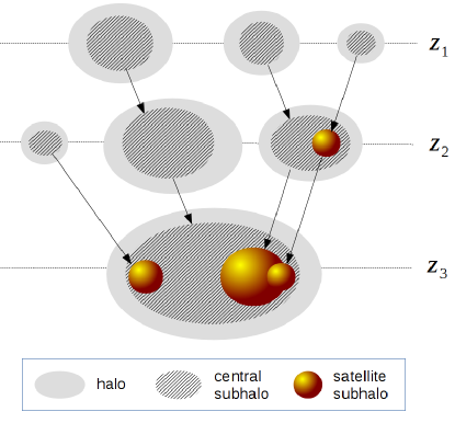
Figure 1: Illustration of a merger tree and the algorithm to find subhalos through tracking. Each horizontal line represents a snapshot labelled by its redshift, with $z_{1}>z_{2}>z_{3}$. As halos merge, satellite subhalos are created as remnants of the progenitors, and can be identified by tracking the progenitor particles to subsequent snapshots and removing unbound particles. For each bound halo, a central subhalo is always defined as the one containing the majority of its bound particles, and is linked to the main progenitor.

2.1 A simple and intuitive merger tree format

Conventional approaches to subhalo finding and merger tree building works by first finding subhalos at each snapshot, then linking them across snapshots. As a result, each subhalo is regarded as a different object and a tree is represented by the links between subhalos at different snapshots. hbt also follows this scheme in tree building, by assigning separate subhalo IDs to subhalos in different snapshots, and recording the progenitor ID for each subhalo, as shown in Fig. 1. Such a representation is also commonly found in popular databases (e.g., the Millennium database) and in a community proposed merger tree format (Thomas et al., 2015), where additional auxilliary links are further provided to facilitate tree walking.

In hbt$+$, we switch to an alternative representation of subhalos and trees by organizing them in terms of tracks, that are native to the tracking algorithm. Each track is the entire evolution history of a subhalo, while a subhalo is a snapshot of a track. This is equivalent to treating a subhalo as a Lagrangian object, which is labelled by a single Lagrangian ID throughout time. Thus a merger tree can be completely specified by a list of tracks associated with halos at each snapshot (e.g., by recording a host halo ID for each track). Fig. 2 shows such an example. Properties of each subhalo at each snapshot can still be added as a local property of the track at different times. This approach essentially flattens the merger tree into a table, which is much more convenient and flexible to store. Such a “track table” is more convenient to query and sample as well. For example, one can directly obtain the progenitor or descendant of a subhalo at any other snapshot by searching for the given track ID, without having to walk the tree snapshot by snapshot. One can also freely remove arbitrarily selected snapshots from the catalogue without having to rebuild the merger tree. As in hbt, the merging hierarchy is propogated to subsequent snapshots to record subhalo groups, so that some subhalos can be satellites of another subhalo.

Once a track ID is created, it persists through all following snapshots. When a subhalo’s mass drops below the mass resolution of the simulation, we use the most bound particle to represent the track. This can be useful for galaxy formation models that place “orphan galaxies” on top of these most bound particles. It can also be used to identify subhalo mergers by identifying the host subhalo of this most bound particle when the subhalo disappears.

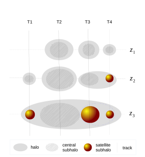
Figure 2: The merger tree in Fig. 1 represented as a list of tracks ($T1$, $T2$, $T3$ and $T4$) grouped by different host halos at each snapshot. The dash-dotted ellipse at $z_{3}$ marks a subhalo group.

2.2 Tracking

Host finding: For each subhalo, its host halo at the next snapshot is simply determined to be the host halo of its most-bound particle. We have checked that such a tracking is robust enough compared with tracking multiple most-bound particles. This is much cleaner than the original hbt treatment that splits the progenitor particles into different hosts, which mostly introduces short-lived noisy tracks (splitter tracks) into the catalogue.

Main progenitor determination: Inside each host halo, the main progenitor is typically selected to be the most-massive one. However, when other progenitors have masses close to the most massive one, such a choice becomes less justified. In this case, we further compare the kinetic energy of the progenitors with respect to the bulk motion of the host halo. Out of all the progenitors whose mass exceeds $2/3$ of the most-massive progenitor mass, the one that has the smallest specific kinetic energy is chosen to be the main progenitor. As we further justify in Equation 2 in Section 2.3, this choice yields the highest total binding energy when all the halo particles are accreted by the main progenitor.

Source subhalo update: An important step for robust tracking is selecting a set of particles–a source subhalo– for each subhalo that are passed to the next snapshot for unbinding (Section 2.3). As is shown in Han et al. (2012), the definition of the source subhalo has to be precise enough so as to avoid too many unbound particles, while at the same time it has to be conservative enough to allow for reaccretion of previously stripped particles. In hbt this is achieved by adaptively chosing a progenitor at some previous snapshot according to the current mass of the subhalo. In this work, we do this in a more flexible way by updating the source continuously. After each unbinding step, source particles are sorted according to binding energy. Less bound particles are excluded, to leave a source subhalo with at most $3N_{\rm bound}$ particles, where $N_{\rm bound}$ is the number of bound particles. This updated source is then passed to the next snapshot for unbinding.

2.3 Stripping

The stripping of mass from subhalos is determined by unbinding.

Reference frame. Unbinding is the process of removing particles whose kinetic energy exceeds their potential energy. To calculate the kinetic energy, a reference frame must be defined, which we choose to be the one that minimizes the total kinetic energy of the subhalo particles. Since

$$K_{\rm tot} =\frac{1}{2}\sum\limits_{i=1}^{N}(\vec{v}_{i}-\vec{v}_{\rm c})^{2}$$ (1)

$$=\frac{N}{2}[(\langle\vec{v}\rangle-\vec{v}_{\rm c})^{2}+(\langle\vec{v}^{2}\rangle-\langle\vec{v}\rangle^{2})],$$ (2)

minimizing the kinetic energy is equivalent to minimizing the distance between the centre velocity and the average velocity vectors, $(\langle\vec{v}\rangle-\vec{v}_{\rm c})^{2}$. When Hubble flow is considered, the distance becomes $(\langle\vec{v}\rangle-\vec{v}_{\rm c}+H\langle\vec{r}-\vec{r}_{\rm c}\rangle)^{2}$. A natural choice is thus the centre of mass frame, centred at $\vec{r}_{\rm c}=\langle\vec{r}\rangle$ with bulk velocity $\vec{v}_{\rm c}=\langle\vec{v}\rangle$. Once unbound particles are removed, we update the reference frame and calculate the binding energies using the gravitational potential from the remaining particles, and unbind again. This process continues until the bound mass converges.

Fast unbinding: The calculation of potential energy during the unbinding iteration is expensive even with a tree code. The majority of the computation time of hbt is spent on unbinding. We introduce two optimizations to speed up this process.

The first optimization is to apply a differential potential update. During every step of the unbinding iteration, the change in potential is due to the removal of unbound particles. When the number of removed particles between two iterations becomes smaller than that of the remaining particles, the potential energy can be efficiently obtained by applying a correction to the potential in the previous iteration, that is, by subtracting the contribution from the removed particles.

For the purpose of unbinding, a very accurate potential energy is not required. Thus we further optimize this step by calculating the potential using a small sample of randomly selected subhalo particles. As we show analytically in Appendix A, the bound density profile of a subhalo can be recovered to percent level accuracy or better over the entire radial range when the mass distribution is sampled with only $1000$ particles. With this algorithm, the potential calculation for all the $N$ particles in the subhalo becomes an $O\left(N\right)$ operation, compared to the $O\left(N\log(N)\right)$ complexity of a tree-code.

Because the potential energy is less accurate in the centre when calculated with a sampled mass distribution, it becomes difficult to select the most bound particle which is a commonly adopted reference frame of a subhalo. To overcome this problem, we further calculate an “inner binding energy” adopting only the potential from the $1000$ most bound particles, and select the most-bound particle thereafter.

We also tried unbinding using a potential estimate that assumes spherical symmetry by binning the mass distribution radially, which can also speed up the calculation significantly. However, such an unbinding tends to fail when spherical symmetry is not a good approximation, such as near pericentric passage where the tidal shear is strong.

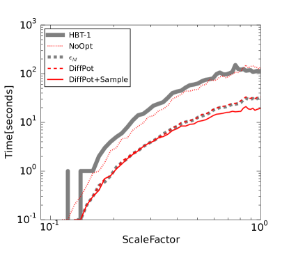
Figure 3: The runtime of hbt$+$ on a test simulation. Different curves show the performance with different levels of optimizations: NoOpt: hbt$+$ with no optimization; DiffPot: hbt$+$ with only differential potential update; DiffPot$+$Sample: hbt$+$ with both differential potential update and sampled potential estimate. For comparison, the thick grey line (HBT-1) shows the timing of hbt, and the dashed grey line ($\epsilon_{M}$) shows the timing of hbt$+$ adopting the same optimization as hbt, which is by relaxing the mass convergence criterion.

In Fig. 3 we show the performance improvement achieved by the various optimizations. We use a test simulation of $270^{3}$ particles with a boxsize of $62.5\,{\rm Mpc}h^{-1}$, run in the same cosmology as that of the Millennium simulation (Springel et al., 2005). The tests are done on a single computational node of the COSMA machine in Durham with $12$ cores. The performance is improved significantly with the differential potential update optimization, and further when the sampled potential estimate is also used. To compare against the performance of hbt, we also run hbt$+$ using the same level of optimization as hbt, which is by terminating the unbinding iteration when the bound mass, $M_{i}$, at iteration $i$ converges with $M_{i+1}/M_{i}>\epsilon_{M}$ where $\epsilon_{M}=0.995$ is the mass precision. The performance difference between hbt and hbt$+$ adopting this common unbinding optimization can be mostly attributed to a change in the central-determination step in Section 2.2. In hbt, the centrals are selected by comparing the bound mass of the progenitors at the current snapshot, which are obtained by one extra unbinding step. By contrast, in hbt$+$, this is done by comparing the progenitor mass at the previous snapshot, together with their current kinetic energies in the host halo frame, avoiding the extra unbinding. Because the $\epsilon_{M}$ optimization introduces similar improvement as the differential potential update optimization, we no longer rely on the $\epsilon_{M}$ optimization in hbt$+$, although this parameter is still available. Overall, the performance is already increased by a factor of $\sim 6$ for this small test simulation, and we expect even higher improvements for larger simulations, given the change in complexity from $O\left(N\log(N)\right)$ to $O\left(N\right)$.

Recursive unbinding As in hbt, the unbinding is done recursively, by unbinding the deepest nested subhalos first and then feeding the stripped particles to their host subhalos for unbinding. This ensures that the particles in each subhalo do not include any bound particles contained in its sub-subhalos, leading to an exclusive mass definition. The subhalo nesting hierarchy is propagated from the merging hiearchy of their progenitor halos.

2.4 Merging

Due to dynamical friction and heating, subhalos could lose their orbital energy and eventually sink to the centre of their host. When the trajectories of two subhalos overlap and evolve together without being separated thereafter, the satellite is trapped at the host centre, and the two subhalos can be defined as having merged. After a merger, tidal stripping ceases to take effect due to the concentric configuration, and the bound mass of the trapped subhalo remains constant until it is heated up by mass accretion or stripped by other halos. We show an example in Fig. 4. We identify trapped mergers by comparing the spatial and velocity separations, $\Delta_{x}$ and $\Delta_{v}$, of the two subhalos with the resolution at the centre of the host subhalo. To estimate the resolution, we use the spatial and velocity dispersion of the 20 most bound particles of the host subhalo, $\sigma_{x}$ and $\sigma_{v}$. Let

$$\delta_{\rm s}=\frac{\Delta_{x}}{\sigma_{x}}+\frac{\Delta_{v}}{\sigma_{v}}.$$ (3)

When $\delta_{\rm s}<2$, the two objects are regarded as merged giving the current numerical resolution. We use the position and velocity of the most bound particle of each subhalo to measure $\Delta_{x}$ and $\Delta_{v}$, so this merger criterion can be interpreted as when the most-bound particles of the two objects cannot be separated in phase space. By default, we merge the trapped subhalo with its host once $\delta_{\rm s}<2$ and only track the most-bound particle thereafter. In Appendix B we provide more information about the distribution of these trapped subhalos for the case when we do not implement this merging criterion.

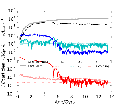
Figure 4: A resolved merger of two subhalos from the Aquarius simulation of a Milky Way sized halo with a particle mass of $2.9\times 10^{5}\,\mathrm{M}_{\odot}h^{-1}$. We show the evolution of mass, separation ($\Delta_{x}$) and relative velocity ($\Delta_{v}$) of the two objects. The spatial and velocity dispersions ($\sigma_{x}$ and $\sigma_{v}$) of the 20 most-bound particles of the host subhalo are also shown; these measure the spatial and velocity resolution at the centre of the halo. The merger of the two objects can be identified with $\delta_{\rm s}<2$, shown as a blue dotted line.

2.5 Parallelization

hbt$+$ comes in two flavours of parallelization: one pure openmp version to be used on a shared memory machine, and one mpi/openmp hybrid version to be used on distributed servers which can also be run in pure mpi mode.

For the openmp version, the parallelization is automatically determined by the symmetry of the workload. When the most massive halo in a snapshot exceeds $10\%$ the total mass of all halos, the parallelization is done inside each halo, by calculating the binding energy of invidividual particles in parallel. Otherwise, the parallelization is done by processing different halos in parallel.

In the current mpi version, the workload is decomposed by dividing the simulation box into spatial grids which are assigned to different computational nodes. Halos and subhalos are then distributed to the grids according to their spatial coordinates. On each node, the computation is then performed in the same way as the openmp version. Because the particles loaded from each halo typically only contain the particle IDs, they must be matched to the particles in the snapshot files to obtain their coordinates and other properties. This is done in parallel by first distributing the snapshots to different nodes according to the particle IDs. The particles in each halo are then split and passed to different nodes according to their IDs. For all the halo particles received on each node, we then sort both the halo particles and the snapshot particles. The sorted halo particles are then matched to the snapshot particles with a batched binary search, which successively narrows down the search range of each particle by the search result of the previous particles. The same is done to query subhalo particles.

2.6 Support for hydrodynamical simulations

The same tracking and unbinding procedure can be applied to hydrodynamical simulations no matter how many types of particles exist in the halo catalogue, although additional routines are needed to handle the creation of particles due to star formation and the destruction of particles due to accretion by black holes. Inside each subhalo, the binding energy of each particle is calculated under the gravitional potential of all types of particles in the subhalo adopting a common reference frame. By default, we do not include the thermal energy of gas particles in the binding energy calculation in order to reflect the instantaneous dynamical state of the system. The effect of thermal energy on the system will be automatically revealed by the instantaneous dynamical state of the system in subsequent snapshots, once the thermal energy is converted to kinetic energy. Technically, however, the code can be configured to output both the binding energy and thermal energy of each particle, so that one can always switch to an alternative binding energy definition including the thermal energy in postprocessing.

3 Tests and application

Previous works have already revealed a few features of hbt, as summarized below:

• The subhalos found by hbt have more extended density profiles compared to the truncated outer density profile typical in configuration space finders, leading to a larger mass estimate in hbt (Han et al., 2012). This difference can be much more significant for massive subhalos.

• hbt easily overcomes the blending problem of subhalos, and successfully recovers subhalos even when a subhalo is deeply embedded in the halo centre (Han et al., 2012; Srisawat et al., 2013).

• hbt maintains consistent link between subhalo progenitor and descendant by construction, and is free from the mass or centre-switching problem in merger tree construction (Srisawat et al., 2013; Behroozi et al., 2015).

However, the mass difference, the blending and mass or centre-switching problems are demonstrated only through case studies of individual objects or through idealized simulations of a single pair of objects. In this section, we aim to investigate these differences statistically using cosmological simulations. In particular, we will compare the distribution of massive subhalos found by hbt$+$ and subfind, in order to understand the systematics in the distribution of these objects, and to shed light on the observed excess of massive subhalos in clusters. In fact, the mass difference also can be understood as a blending problem that obscures the outskirts of a subhalo, while the mass or centre-switching is created by partial or total obscuration of the subhalo in the merger tree. It is thus natural to expect that all three issues are significant for massive subhalos.

3.1 Simulations

We make use of two simulations in this section. The first is the Millennium-II simulation (Boylan-Kolchin et al., 2009) in the $\Lambda$CDM cosmology with $\Omega_{\rm m}=0.25$ and $\sigma_{8}=0.9$. It resolves $2160^{3}$ particles in a cubic box of $100~{}{\rm Mpc}h^{-1}$ on each side, with a particle mass of $6.89\times 10^{6}\,\mathrm{M}_{\odot}h^{-1}$. The other simulation is a zoomed in simulation of a Milky Way sized halo from the Aquarius simulation set (Springel et al., 2008a) with the same cosmology as Millennium-II. The Aquarius set consists of several Milky Way sized halos each simulated with a series of resolutions. We mainly use the first halo simulated at the second highest resolution level, which we call halo AqA2 hereafter. It has a particle mass of $10^{4}\,\mathrm{M}_{\odot}h^{-1}$ in the high resolution region, corresponding to $\sim 10^{8}$ particles resolved in the main halo.

The Millennium-II simulation provides a large sample of halos to study the average distribution of subhalos in host halos of different mass. Most importantly, it allows us to study the distribution of massive subhalos statistically, which is impossible with a single host halo due to the rarity of massive subhalos. We will study three aspects of the subhalo population: the final subhalo mass, the peak subhalo mass (i.e., the maximum mass attained by a subhalo over its entire history), and the location inside the host halo. As we will show, combining the final and peak subhalo mass function allows us to assess the quality of the merger tree statistically, which is further demonstrated in a side-by-side comparison of the merger trees of the AqA2 halo.

3.2 The subhalo mass function

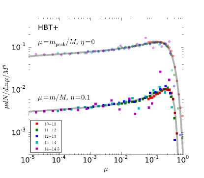
Figure 5: The peak and final subhalo mass functions in Millennium-II halos, normalized by $M^{\eta}$ where $M$ is the host halo mass. $\eta$ and the mass variable $\mu$ are specified in the figure for the peak and final mass functions respectively. Data points and lines of different colour represent different host halo mass bins, as listed in the legends in terms of $\log(M/{\mathrm{M}_{\odot}h^{-1}})$. The light thick lines are the fits of Eqn (4), with best-fit parameters listed in Table 1 (200Crit rows). The results for other virial definitions are qualitatively similar.

It is well known that the subhalo mass function follows a simple power-law behaviour at the low mass end, $\frac{\mathrm{d}N}{\mathrm{d}lnm}\propto m^{-\alpha}$, with $\alpha\approx 0.9$ (e.g., Gao et al., 2004). It has also been shown that the slope of $\alpha$ is conserved between the unevolved and evolved subhalo mass function (Han et al., 2016). In Fig. 5 we show the subhalo mass functions from the Millennium-II simulation. Both the evolved mass function and the unevolved mass functions are shown, which we call the final and peak subhalo mass functions respectively. These functions are computed as follows. For each host halo, we identify all the branches that are currently located within its virial radius according to the position of the most bound particle of each branch. After that, the evolved mass function is defined as the distribution of the final subhalo mass of these branches, and the unevolved mass function is defined as the distribution of their peak bound masses. Both surviving and disrupted branches contribute to the peak-mass function.

Table 1: Fits to the subhalo mass functions of the form Equation (4). We show the results for three different definitions of the host halo mass $M$, corresponding to spherical overdensities of 200 times the critical density (200Crit, our default choice in this work), 200 times the mean mass density (200Mean) of the universe and that given by the spherical collapse model (Virial). The abundances are computed inside the radius of the corresponding spherical overdensity. $m$ and $m_{\rm peak}$ are the final and peak mass of the subhalo.

Host Halo Definition	$\mu$	$a_{1}$	$\alpha_{1}$	$a_{2}$	$\alpha_{2}$	$b$	$\beta$	$\eta$
200Crit	$m/M$	0.0055	0.95	0.017	0.24	24	4.2	0.1
	$m_{\rm peak}/M$	0.11	0.95	0.20	0.30	7.6	2.1	0
Virial	$m/M$	0.0072	0.95	0.017	0.26	54	4.6	0.1
	$m_{\rm peak}/M$	0.11	0.95	0.32	0.08	8.9	1.9	0
200Mean	$m/M$	0.0090	0.95	0.055	0.16	36	3.2	0.1
	$m_{\rm peak}/M$	0.11	0.95	0.64	-0.20	11	1.8	0

With the large sample of halos, we are able to well resolve the high mass end of the mass function. Both distributions are well fitted by a double Schechter function of the form

$$f(\mu)\equiv\frac{\mathrm{d}N}{\mathrm{d}\ln\mu}$$

$$=\left(\frac{M}{10^{10}\mathrm{M}_{\odot}h^{-1}}\right)^{\eta}\left(a_{1}\mu^{-\alpha_{1}}+a_{2}\mu^{-\alpha_{2}}\right)\exp\left(-b\mu^{\beta}\right),$$ (4)

where $\mu$ is the ratio of the final (peak) mass of the subhalo to the host halo mass. By default, we adopt the virial definition corresponding to a spherical overdensity of 200 times the critical density of the universe. However, we list the best-fit parameters for three common virial definitions in Table 1. The first power-law component in Equation (4) describes the low mass end behaviour of the mass function, while the second component is necessary to fit the shoulder at $\mu>0.1$. Note that fitting the low mass end slope can be tricky depending on the weights given to the data points, the available mass range that is trusted to have converged, and the functional form adopted to describe the high mass end behaviour. Thus we refrain from fitting this slope. Instead, we fix $\alpha_{1}=0.95$ according to the result of Han et al. (2016) using much higher resolution data. As shown in Fig. 5, such a choice is well supported by the data.

Despite the apparently different parameter values, the peak-mass function depends only weakly on the virial definition. Consistent with previous studies (van den Bosch et al., 2005; Giocoli et al., 2008), the peak-mass function is independent of the host halo mass. On the other hand, the final mass function scales with the host halo mass as $M^{0.1}$ in the host mass range probed by our simulation. This is consistent with the expectation that more massive halos are younger, thus possessing a higher mass fraction in subhalos. Overall, the peak mass and final mass functions have similar shapes, while the presence of a shoulder at $\mu>0.1$ is more prominent in the final mass function. In Fig. 6 we show the ratio between the two fitted mass functions. For Milky Way sized and cluster sized halos, the ratio is around $0.1$ at the low mass end, consistent with the findings of Han et al. (2016). If tidal stripping of the subhalos is independent of subhalo mass, then the peak mass and final mass functions are expected to have the same shape. At the high mass end, however, there is a peak in the ratio, indicating that the massive satellites are less stripped than the low mass ones. This is not surprising because when the satellite mass is comparable to the mass of the host halo, the tidal force from the host becomes less important compared with the self-gravity of the satellite.

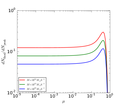
Figure 6: The ratio between the final mass and peak-mass subhalo mass functions, for different host halo masses ($10^{14}$, $10^{12}$ and $10^{10}\,\mathrm{M}_{\odot}h^{-1}$ from top to bottom).

3.3 The radial distribution of subhalos

The peak in Fig. 6 can be further understood by reference to the spatial distribution of the subhalos. As shown in Fig. 7, the radial distributions of subhalos of different relative mass have the same shape near the virial radius, where the subhalos are barely affected by tidal stripping and are expected to follow the host halo density profile (Han et al., 2016). At smaller radii, however, massive subhalos have a steep profile while less massive subhalos are depleted at the centre. This pattern is a consequence of both dynamical friction and tidal stripping. The former is more important for massive subhalos, making them sink to smaller radii. At the same time, tidal stripping is less effecient for massive subhalos, and even more so at the centre of the host when the satellite largely overlaps with the host, thus failing to eliminate these objects.

Being free from tidal stripping, the relative abundance of subhalos near the virial radius is expected to follow the peak-mass function, i.e., $n(R_{200},m)\propto f_{\rm peak}(m)$. The subhalo mass function within the virial radius is simply an integral of subhalo abundance inside $R_{200}$,

$$f_{\rm final}(\mu) =\int_{0}^{R_{200}}n(r,m)\mathrm{d}^{3}r$$ (5)

$$=n(R_{200},m)\int_{0}^{R_{200}}\frac{n(r,m)}{n(R_{200},m)}\mathrm{d}^{3}r$$ (6)

$$\propto f_{\rm peak}(m)\int_{0}^{R_{200}}\frac{n(r,m)}{n(R_{200},m)}d^{3}r.$$ (7)

The cuspier radial profile for massive subhalos leads to an increase in the integral of the relative profile in Equation (7). As a result, the ratio between the final mass and peak-mass profiles is also higher for massive subhalos. Note that the data in Han et al. (2016) only probes the subhalo distribution at $m/M<10^{-3}$ where this effect is smaller and further suppressed by the use of a different subhalo finder, as we show explicitly in Section 3.4.1 below. In a follow-up paper, we will extend the model of Han et al. (2016) to study these distributions in detail.

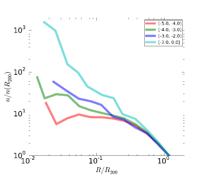
Figure 7: The radial distribution of subhalos in host halos of $10^{13}-10^{14}\,\mathrm{M}_{\odot}h^{-1}$. The subhalos are binned in $\log(m/M)$ as labelled. The profiles are normalized by their values at the host virial radius, $R_{200}$. For reference, the gravitational softening of the simulation is about $0.002\,R_{200}$ for these host halos.

3.4 Comparison with other works

3.4.1 Direct comparison with subfind

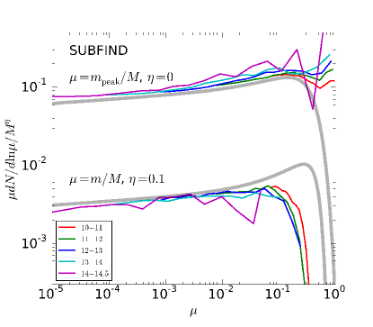
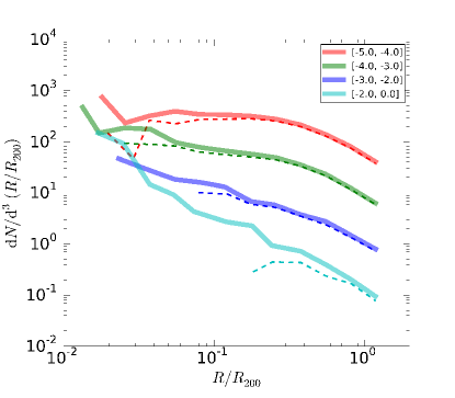
Figure 8: Left: The peak mass and final subhalo mass functions for subfind and dtree. The thick grey lines are fits to that of hbt$+$ subhalos (same as in Fig. 5). The thin lines with different colours are subfind$+$dtree results in host halos of different masses (labelled by $\log(M/M_{\odot}h^{-1})$). Right: the radial profile of subfind subhalos (dashed lines) compared with that of hbt$+$ subhalos (solid lines). The host halo mass and the subhalo mass bins are identical to those in Fig. 7, except that the profiles are not normalized at $R_{200}$ in order to compare the relative amplitude of the two datasets.

In Fig. 8 we compare our mass functions and radial distributions with that found by subfind (Springel et al., 2001). To compute the peak-mass function, we use the merger tree built by the Durham merger tree code dtree (Jiang et al., 2014). dtree has been developed with efforts to overcome halofinder pitfalls that could cause missing links or frequent switching of links, and is the default $N$-body merger tree used by the galform semi-analytic models of galaxy formation (Bower et al., 2006). We extend the merger tree by tracking the most bound particle after termination of a branch, so that the peak-mass function can be computed in the same way as our code.

As in hbt (Han et al., 2012), our final mass function is $\sim 10\%$ above that of the subfind at the low mass end. At the high mass end, however, the difference is dramatic, corresponding to a factor of $2-3$ difference in subhalo mass or an order of magnitude difference in abundance. This has been pointed out as a problem of subfind through comparison with some other halo finders (including rockstar and surv, van den Bosch & Jiang, 2016) for these massive subhalos.

In the right panel of Fig. 8, we explore this difference in the spatial distribution of subhalos. In the outer halo, our subhalos are slightly more abundant, which can be understood as our subhalos being slightly more massive. The overall shape of the distributions are still quite consistent with each other. In the inner halo, however, subfind shows a deficiency of subhalos compared with our result, which is most significant for more massive subhalos. This can be understood as a reflection of the ‘blending problem’ exhibited by configuration space subhalo finders: when a subhalo overlaps with the host halo, it is difficult to separate it from the host using only density information. It is easy to understand that this issue is more severe for larger subhalos.

The deficiency of massive subhalos near the centre of the host halo in catalogues constructed using subfind explains, at least in part, the disagreement noted by Schwinn et al. (2017) and Natarajan et al. (2017) between the distrubtion of subhalos identified using subfind in $\Lambda$CDM simulations and the distribution of subhalos inferred from lensing studies in galaxy clusters. Mao et al. (2017) have argued that the mismatch between the simulation result of Millennium-XXL (Angulo et al., 2012) and the lensing results of Jauzac et al. (2016); Schwinn et al. (2017) is also affected by the use of different masses in the comparison: subfind masses in the simulation but projected aperture masses from lensing that also include mass contributions from the host. Even with the use of deblended subhalo mass estimates in the strong lensing analysis of Natarajan et al. (2017), however, the observed spatial distribution of massive subhalos is still found to be more centrally concentrated than that from the subfind catalogues of the Illustris simulations (Vogelsberger et al., 2014), which can be attributed to this radial-dependent blending issue in the subfind catalogues.

In contrast to the final mass function, the peak-mass function from subfind$+$dtree is systematically above ours. Together with the lower final mass function, this means more branches are produced in the merger tree of subfind$+$dtree. As we will show explicitly in Section 3.5, this difference can be attributed to broken branches associated with missing links and the switching of subhalo masses in subfind$+$dtree.

3.4.2 Comparison with fitting functions and the low mass end slope

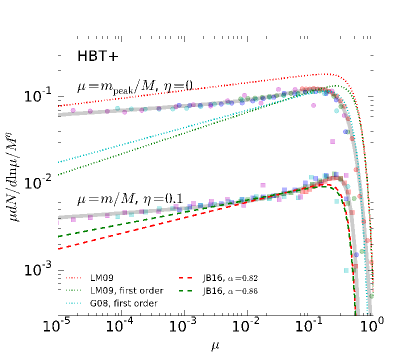
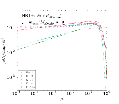
Figure 9: The subhalo mass functions compared with fitting functions in previous works. As in Fig. 5, the data points are results from our code, with different colors representing different host halo mass bins. The squares and circles show the peak mass and final subhalo mass functions respectively. The thick lines are fits to the data points as listed in Table 1. The peak-mass function is compared with the fitting functions of Li & Mo (2009) for all the subhalos and first-order subhalos, as well as with the fit of Giocoli et al. (2008) for first-order subhalos. The final mass function is compared with the fitting function of Jiang & van den Bosch (2016) and van den Bosch & Jiang (2016) which are calibrated using the ROCKSTAR halo finder. In the left panel, we adopt the “Virial” definition for both host mass and radius. In the right panel, the host halo mass is defined according to the “200Crit” definition while the host halo radius is defined according the “200Mean” definition.

In Fig. 9 we compare our results against a few fitting functions in the literature. In the left panel, we have switched to the same definition of virial quantities (“Virial” as in Table 1) as in Giocoli et al. (2008); Jiang & van den Bosch (2016); van den Bosch & Jiang (2016) when computing the mass functions. The model of Jiang & van den Bosch (2016) is a semi-analytical model that evolves progenitor halos generated from extended Press-Schechter merger trees according to an empirical average mass stripping rate. Their model is calibrated against rockstar subhalos from the Bolshoi (Klypin et al., 2011) and MultiDark (Prada et al., 2012) simulations, and the resulting subhalo mass function is fitted using a Schechter function. The normalization of the mass function is predicted from the dynamical age of the host halo, which we find can be equivalently fitted with a power-law in the mass range $10^{10}-10^{15}\mathrm{M}_{\odot}h^{-1}$ for the concordance cosmology, consistent with our scaling in Table 1. For the purpose of comparison with our results, the final fitting function of the Jiang & van den Bosch (2016) model can then be summarized as

$$\frac{\mathrm{d}N}{\mathrm{d}\ln\mu}=a\left(\frac{M}{10^{10}\mathrm{M}_{\odot}h^{-1}}\right)^{\eta}\mu^{-\alpha}\exp\left(-b\mu^{\beta}\right),$$ (8)

with $a=0.014$, $\eta=0.1$, $\alpha=0.82$, $b=50$, $\beta=4$ according to Jiang & van den Bosch (2016), and slightly different parameters $a=0.012$, $\alpha=0.86$ in van den Bosch & Jiang (2016). Our results are quite consistent with their fitting function with $\alpha=0.86$ in the mass range $10^{-3}<\mu<10^{-1}$. At the high mass end, our data shows a higher shoulder around $\mu=0.3$, indicating that the mass stripping rate of the most massive subhalos differs from the average mass stripping rate of low mass ones in the framework of the Jiang & van den Bosch (2016) model. At the very low mass end, our data clearly support a slope higher than $\alpha=0.86$. While van den Bosch & Jiang (2016) argued that their data is in contradiction with a low mass end slope of $\alpha=0.95$, our results suggest that their conclusion is caused by the limited mass range in their data ($\mu>10^{-3}$). The local slope is an increasing function of subhalo mass due to the decrease in tidal stripping efficiency at the high mass end, and the asymptotic $\alpha$ is still consistent with $0.95$ down to $\mu\sim 10^{-5}$.

For the peak-mass function, Giocoli et al. (2008) has measured the first-level unevovled mass function, that is, the mass distribution of progenitors that fall directly into the host halo (instead of being accreted as a satellite of another infalling halo). At the high mass end, the peak-mass function is dominated by these first-level progenitors, and our measurement agrees very well with that of Giocoli et al. (2008). At the low mass end, higher level contributions become more important, and the Giocoli et al. (2008) fit falls below our measurement. Li & Mo (2009) measured both the first-level and all level unevolved mass function, which have been used in Jiang & van den Bosch (2014, 2016) as benchmarks to calibrate Monte-Carlo merger trees from extended Press-Schechter theories. Their results lie mostly above our measurements. However, it should be noted that Li & Mo (2009) adopted a somewhat peculiar combination of the mass and spatial extension of a host halo. Their merger trees are based on Friends-of-Friends (FoF) halos, while the host halo mass is defined as $M_{\rm 200Crit}$ corresponding to a spherical overdensity that is 200 times the critical density of the universe. To make a better comparison, in the right panel of Fig. 9 we compute the peak mass function inside $R_{\rm 200Mean}$, which is expected to be closest to the size of a Friends-of-Friends halo, while adopting $M_{\rm 200Crit}$ as the host halo mass. Such a combination leads to a mass function that is closer to the Li & Mo (2009) results, but still lower at the high mass end. This can be further attributed to the fact that they rely on Friends-of-Friends halos to build their merger trees. In this case, halos that are temporarily linked together and subhalos that have been ejected from the host can both contribute to the progenitor mass function. The situation can become even worse if these objects fall back into the host and are counted multiple times (Benson, 2017). In contrast, our approach of selecting branches located inside the final virial radius produces a progenitor population that can be unambiguiously compared against the final mass function inside the virial radius. Due to these complications, the Li & Mo (2009) results should be quoted with caution in future analytical studies.

3.5 The persistence of tracks

To further investigate the difference in the peak-mass function between subfind$+$dtree and hbt$+$, we carry out a detailed study focusing on a single high resolution halo, AqA2 from the Aquarius simulation set. Fig. 10 shows the peak mass computed from our code and that from subfind$+$dtree. Consistent with Fig. 5, the peak-mass function from subfind$+$dtree is higher than ours. According to whether the descendant subhalo at $z=0$ is still resolved, we decompose the peak-mass function into a surviving and a disrupted component. The peak-mass functions of surviving subhalos agree well with each other, meaning that both codes have identified the same population of final subhalos. On the other hand, the disrupted peak-mass functions can differ up to a factor of $2$, with subfind$+$dtree having more disrupted branches.

In the $(r,m_{\rm peak})$ plane, we have identified some of these extra branches that exists in subfind$+$dtree but not in hbt$+$. Fig. 11 shows the mass evolution history of the three most massive branches (B1, B2, B3) selected this way. Correspondingly, we have also identified branches in hbt$+$ that best match the selected branches in orbital and mass evolution. Interestingly, these branches are related to two major merger events that happened to the host halo. In the subfind$+$dtree case, the B1, B2, and B3 branches all temporarily become the most massive branch in the host at some stage, and then get disrupted almost immediately after that. The final central subhalo emerges abruptly from inside the host halo, as shown by the B1-1 branch. In contrast, the corresponding T2 and T3 branches in hbt$+$ remain as less massive branches than T1 after merger until they are fully disrupted. The T1 branch remains as the most massive branch in the host halo untill the final time. In Fig. 12, we visuallize this evolution as a track table, where an additional branch, B4 (T4), is included to show the major merger with B3 (T3) that leads to the strange mass growth in B3. In the hbt$+$ case, the central and satellite subhalos are tracked consistently and persistently, while the subfind$+$dtree tree suffers a few switches in the mass and in the central-satellite determination, as well as a broken link that fragmented B1-1 from B1. The switching problem leads to an overestimate of the peak mass, while the broken links create extra progenitor branches. Both of these lead to an overestimate of the peak-mass function.

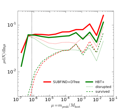
Figure 10: The peak-mass function (solid line) of tracks in Aquarius halo A2, decomposed into disrupted and surviving populations (dotted and dashed lines). The red and green colours show the results of subfind$+$dtree and hbt$+$ respectively.

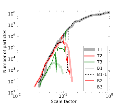
Figure 11: The mass evolution of the central subhalo of AqA2. The thin lines show the mass evolution history of subhalos that are identified as the central subhalo of AqA2 at different times according to subfind$+$dtree. The thick lines show the corresponding branches as identified by hbt$+$.

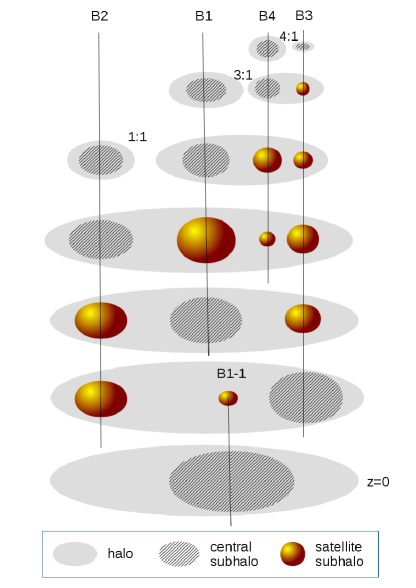
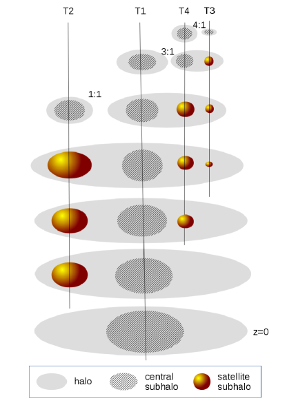
Figure 12: The major merger history of halo AqA2 as resolved by subfind$+$dtree (left) and hbt$+$ (right). The ratios next to halos list the mass ratio of the progenitor halos just before the merger. Each track (vertical lines) terminates after the disruption of the subhalo. For illustration purpose, only the snapshots of interests are plotted.

4 Summary and conclusion

We have presented an improved version of the original hbt algorithm of Han et al. (2012) that tracks halos through time to find subhalos and build merger trees. A series of improvements are implemented, including:

• Treatment of subhalos as Lagrangian objects and organization of the merger tree as a table of tracks. This allows intuitive and flexible storage and retrieval of subhalos and trees.

• Significant improvement in speed. This is made possible by a physically motivated yet simple algorithm for the identification of the main progenitor halo and a refined unbinding algorithm with a complexity of $O\left(N\right)$ compared to the $O\left(N\log N\right)$ complexity of a plain tree code.

• Detection and merging of trapped subhalos. These are massive satellites that sink to the centre of their host halo and remain there without being disrupted, leading to pairs of subhalos that overlap in their orbit while remaining individually self-bound. We have developed a prescription to detect such pairs and merge the trapped satellite.

• Support for distributed computation through mpi.

• Support for hydrodynamical simulations.

The code has been rewritten in C++ with user friendly configuration options, as well as HDF5 output format that allows direct postprocessing with other software. The source code is publicly available at https://github.com/Kambrian/HBTplus and http://icc.dur.ac.uk/data/.

As an illustration we applied the new code to a study of the distribution of subhalos and tested the persistence of merger trees in the Millennium-II simulation and in one of the Aquarius project simulations. In contrast to previous studies that fit the mass functions with a single Schechter function, we find that both the final and peak-mass subhalo mass functions are well fitted by a double Schechter function (Eq. (4)) with similar shapes. These mass functions harden towards the high mass end before falling off exponentially. The hardening is most significant in the final mass function, reflecting an inefficiency of tidal stripping of massive subhalos. This also reflects our finding that the radial distribution of massive subhalos is more concentrated than the universal radial profile of low mass ones, due to stronger dynamical friction and weaker tidal stripping. The detection of this hardening requires the ability to identify subhalos in the inner regions of the host halo, which hbt$+$ does, but which subhalo finders that work in configuration space alone have difficulty identifying. Recent lensing observations of galaxy clusters have resulted in reports of discrepancies in the observed subhalo distribution compared to that of $\Lambda$CDM predictions, including the excess of massive subhalos reported by Jauzac et al. (2016) and Schwinn et al. (2017) and the more concentrated subhalo radial distribution reported by Natarajan et al. (2017). These discrepancies can be explained, at least in part, by the blending problem present in the Millennium-XXL and Illustris subfind catalogues used in their comparisons.

The hardening of the subhalo mass function at the high mass end means that single power-law fits to the mass function are inadequate. From our hbt$+$ subhalo catalogues constructed from the Millennium-II simulation, we find that, when the entire mass function is fitted with a double Schechter function, the low-mass end slope (down to $m/M_{\rm host}=10^{-5}$) is consistent with a power-law exponent, $\alpha=0.95$.

We have demonstrated that the peak-mass function, or the ratio between the peak mass and final mass functions, are good statistics to test the quality of merger trees. The existence of broken or false links in the trees introduces extra branches and inflates the peak-mass function, which can be overestimated by as much as a factor of 2 in an complex merger tree built from subfind subhalos, as a result of the ‘blending’ and ‘mass or centre-switching’ problems that are present in the latter. This issue is important for studies that focus on the remnants of the most massive progenitors in a halo, such as studies of streams in the Milky Way halo. It also has important implications for abundance matching models that match galaxies to simulated merger trees using peak masses: the peak mass function inflated by broken and false links could lead to false matches of galaxies to broken branches, subsequently biasing the inferred properties of massive satellite galaxies. In contrast, our algorithm is robust against these problems by design. It is able to track the tree branches persistently, and recovers a higher final mass function, as well as a lower and universal peak-mass function.

Appendix A Sampling noise in unbinding

Consider a singular isothermal sphere sampled with $N$ particles out to a truncation radius $r_{\rm max}$. Expressed in the dimensionless radius $\tilde{r}=r/r_{\rm max}$, the cumulative number density profile of the halo particles is $N(<\tilde{r})=N\tilde{r}$. Assuming Poisson fluctuations in the particle counts at each radius, the uncertainty in the estimated potential can be obtained as

$$\delta_{\psi}(r) \equiv\frac{\sigma_{\psi}(r)}{|\psi(r)|}$$ (9)

$$=\frac{\sqrt{\frac{N(r)}{r^{2}}+\int_{r}^{r_{\rm max}}\frac{\mathrm{d}N(R)}{R^{2}}}}{\frac{N(r)}{r}+\int_{r}^{r_{\rm max}}\frac{\mathrm{d}N(R)}{R}}$$ (10)

$$=\frac{1}{\sqrt{N}}\frac{\sqrt{2/\tilde{r}-1}}{1-\ln\tilde{r}}.$$ (11)

At $r=r_{\rm max}$, the uncertainty is the smallest with $\delta_{\psi}(r_{\rm max})=1/\sqrt{N}$. The radial dependence of this Poisson noise is shown in Fig. 13.

The uncertainty of the bound density profile due to Poisson noise can be estimated as

$$\delta_{\rho}(r) \equiv\frac{\sigma_{\rho}(r)}{\rho(r)}$$ (12)

$$=\frac{\int_{\sqrt{2|\psi|}}^{\sqrt{2(|\psi|+\sigma_{\psi})}}\exp\left(-\frac{v^{2}/2+\psi}{\sigma^{2}}\right)d^{3}v}{\int_{0}^{\sqrt{-2\psi}}\exp\left(-\frac{v^{2}/2+\psi}{\sigma^{2}}\right)d^{3}v}$$ (13)

$$=\frac{f(b)}{f(a)}-1,$$ (14)

where $f(x)=\sqrt{\pi}\mathrm{erf}(x)-2e^{-x^{2}}x$, $a=\sqrt{|\psi|/\sigma^{2}}=\sqrt{2(1-\ln\tilde{r})}$, $b=\sqrt{(|\psi|+\sigma_{\psi})/\sigma^{2}}=\sqrt{2(1-\ln\tilde{r})(1+\delta_{\psi}(r))}$, and $\sigma^{2}$ is the one-dimension velocity dispersion of the halo. This is plotted in Fig. 14 for a few different sample sizes, $N$. For $N=10^{3}$, the density profile can be recovered to percent level accuracy or better over the entire radial range.

Even though the potential estimate is less accurate at smaller radii, the unbinding of the particles is almost unaffected by Poisson noise at these radii. This is because the potential is much deeper at small $r$. Given the constant velocity dispersion in the isothermal sphere, most of the particles at a small $r$ are tightly bound, making the unbinding insensitive to the accuracy in potential. This is also true for NFW haloes, in which the velocity dispersion is known to eventually decrease towards the halo centre.

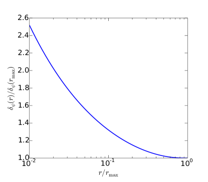
Figure 13: The radial dependence of the Poisson noise in the estimated potential for an isothermal sphere sampled with particles. The noise increases as the radius decreases.

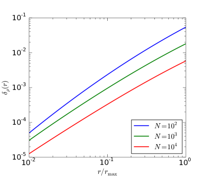
Figure 14: The relative uncertainty in the self-bound density profile due to Poisson noise in the potential, for an isothermal sphere sampled with $N$ particles.

Appendix B Trapped subhalos

Massive satellites are likely to sink to the centre of their host halo without getting disrupted. During this process, the orbital energy of the central-satellite pair is converted to the internal energy of each subhalo, and the satellite is trapped in the centre thereafter. To see that these satellites are indeed a distinct population, in Fig. 16 we show the distribution of satellites according to their position and velocity offset from their host subhalos. Here $\delta_{x}=\Delta_{x}/\sigma_{x}$, where $\Delta_{x}$ is the separation of the satellite from its host subhalo, and $\sigma_{x}$ is the position dispersion of the $20$ most-bound particles in the host subhalo. Similarly, $\delta_{v}=\Delta_{v}/\sigma_{v}$ is the normalized velocity offset. It is obvious that the satellites show a bimodal distribution in this plane, with the trapped subhalos clustered around $(\delta_{x},\delta_{v})=(1,1)$, consistent with them being draw from the most bound particles in the host subhalo. Note that in this test we have not merged the trapped subhalos in order to make this plot, but only tag them as trapped as soon as they reach $\delta=\delta_{x}+\delta_{v}<2$ in their orbital evolution.

In Fig. 15 we show the distribution of $\sigma_{x}$ and $\sigma_{v}$ as a function of subhalo mass. When using the peak mass as a proxy of satellite mass, the distributions are quite similar for central and satellites. $\sigma_{x}$ approaches the softening of the simulation in well resolved subhalos, while it is generally bigger for subhalos with less than $10^{3}$ particles. The velocity scale $\sigma_{v}$, however, increases with subhalo mass, since more massive objects are dynamically hotter. The median relation can be well fitted by

$$\sigma_{v}=\left(-3.2+7.4\ln N\right){{\rm km}\,{\rm s}^{-1}},$$ (15)

where $N$ is the number of particles in the subhalo. However, we caution that the above fitting formula may not be applicable to simulations with different resolutions.

The mass functions of trapped subhalos are shown in Fig. 17. These objects are mostly massive objects with $m/M>0.1$, and they evolve only mildly since infall, with the peak and final mass functions differing by a factor of $2\sim 3$. Note that these trapped subhalos have already been removed in the figures in the main text of the paper. One might wonder whether the over-abundance of subhalos at the high mass end in our result is contaminated by trapped subhalos that are not completely removed. Since the trapped subhalos are mostly located within $2\sigma_{x}$, they do not contaminate the radial profiles in Fig. 7 and Fig. 8 in $10^{13}\,\mathrm{M}_{\odot}h^{-1}$ halos (corresponding to more than $10^{6}$ particles) where the softening is around $0.002\,R_{200}$. Subsequently, the existence of the flattening in the subhalo mass function is robust against contaminations from trapped subhalos as discussed in Section 3.3.

These merged subhalos represent the case when numerical resolution of the simulation is no longer able to separate the subhalo from its host. We have carried out a test using a lower resolution simulation and found that the mass functions of the merged subhalos seem to have converged (though noisily). Even so, whether the galaxies in the trapped subhalos have merged with their central galaxy is a different problem.

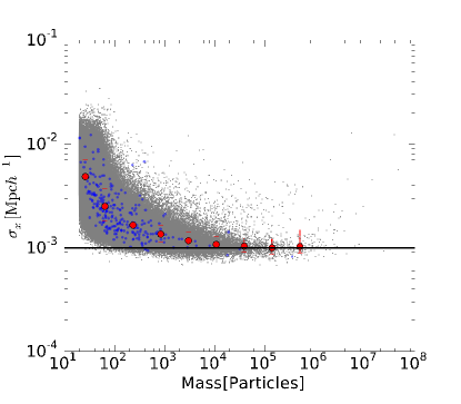
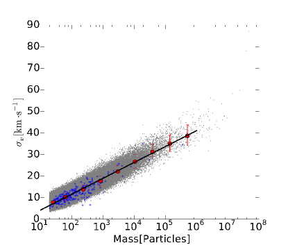
Figure 15: The position and velocity resolution in subhalos of different masses in Millennium-II. The grey dots are the results for central subhalos while the blue dots are those for satellites. In this figure we use the peak mass of a satellite as its mass. For clarity, only $1/10$ of the central subhalos and $1/10000$ of the satellite subhalos are plotted. Filled circles with errorbars show the median and $\pm 1\sigma$ percentiles of the distributions. In the top panel, the horizontal solid line marks the force softening of the simulation. In the bottom panel, the black solid line shows a fit (Eq 15) to the median relation.

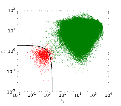
Figure 16: The distribution of satellites in the $(\delta_{x},\delta_{v})$ plane at $z=0$ in Millennium-II. We select satellites that are still resolved and whose host subhalo has more than $10^{4}$ particles. $\delta_{x}$ and $\delta_{v}$ are the position and velocity offset of the satellite from its host subhalo, normalized by the position and velocity dispersions at the host centre respectively. The red dots are satellites tagged as trapped while the green dots are the remaining ones. The black line marks $\delta_{x}+\delta_{v}=2$, the critical curve used to identify trapped subhalos in the merger history.

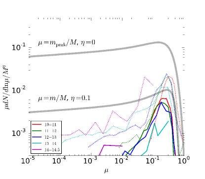
Figure 17: The mass distribution of trapped subhalos that still survive at $z=0$ in Millennium-II. The thick grey lines are the same as in Fig. 5 showing the fitted peak and final mass functions for normal subhalos. The coloured lines show the mass functions of trapped subhalos in different host halo mass bins (as labelled by $\log[M/\mathrm{M}_{\odot}h^{-1}]$), with the solid and dotted lines showing the final and peak mass functions respectively.

References

- Angulo et al. (2012) Angulo R. E., Springel V., White S. D. M., Jenkins A., Baugh C. M., Frenk C. S., 2012, MNRAS, 426, 2046, arXiv:1203.3216
- Avila et al. (2014) Avila S. et al., 2014, MNRAS, 441, 3488, arXiv:1402.2381
- Behroozi et al. (2015) Behroozi P. et al., 2015, MNRAS, 454, 3020, arXiv:1506.01405
- Behroozi et al. (2013) Behroozi P. S., Wechsler R. H., Wu H.-Y., 2013, ApJ, 762, 109, arXiv:1110.4372
- Benson (2017) Benson A. J., 2017, MNRAS, 467, 3454, arXiv:1610.01057
- Bower et al. (2006) Bower R. G., Benson A. J., Malbon R., Helly J. C., Frenk C. S., Baugh C. M., Cole S., Lacey C. G., 2006, MNRAS, 370, 645, astro-ph/0511338
- Boylan-Kolchin et al. (2009) Boylan-Kolchin M., Springel V., White S. D. M., Jenkins A., Lemson G., 2009, MNRAS, 398, 1150, arXiv:0903.3041
- Davis et al. (1985) Davis M., Efstathiou G., Frenk C. S., White S. D. M., 1985, ApJ, 292, 371
- Elahi et al. (2011) Elahi P. J., Thacker R. J., Widrow L. M., 2011, MNRAS, 418, 320, arXiv:1107.4289
- Gao et al. (2004) Gao L., White S. D. M., Jenkins A., Stoehr F., Springel V., 2004, MNRAS, 355, 819, astro-ph/0404589
- Ghigna et al. (1998) Ghigna S., Moore B., Governato F., Lake G., Quinn T., Stadel J., 1998, MNRAS, 300, 146, astro-ph/9801192
- Giocoli et al. (2010) Giocoli C., Tormen G., Sheth R. K., van den Bosch F. C., 2010, MNRAS, 404, 502, arXiv:0911.0436
- Giocoli et al. (2008) Giocoli C., Tormen G., van den Bosch F. C., 2008, MNRAS, 386, 2135, arXiv:0712.1563
- Han et al. (2016) Han J., Cole S., Frenk C. S., Jing Y., 2016, MNRAS, 457, 1208, arXiv:1509.02175
- Han et al. (2012) Han J., Jing Y. P., Wang H., Wang W., 2012, MNRAS, 427, 2437, arXiv:1103.2099
- Jauzac et al. (2016) Jauzac M. et al., 2016, MNRAS, 463, 3876, arXiv:1606.04527
- Jiang & van den Bosch (2014) Jiang F., van den Bosch F. C., 2014, MNRAS, 440, 193, arXiv:1311.5225
- Jiang & van den Bosch (2016) Jiang F., van den Bosch F. C., 2016, MNRAS, 458, 2848
- Jiang et al. (2014) Jiang L., Helly J. C., Cole S., Frenk C. S., 2014, MNRAS, 440, 2115, arXiv:1311.6649
- Klypin et al. (1999) Klypin A., Gottlöber S., Kravtsov A. V., Khokhlov A. M., 1999, ApJ, 516, 530, astro-ph/9708191
- Klypin et al. (2011) Klypin A. A., Trujillo-Gomez S., Primack J., 2011, ApJ, 740, 102, arXiv:1002.3660
- Knebe et al. (2011) Knebe A. et al., 2011, MNRAS, 415, 2293, arXiv:1104.0949
- Knollmann & Knebe (2009) Knollmann S. R., Knebe A., 2009, ApJS, 182, 608, arXiv:0904.3662
- Lacey & Cole (1994) Lacey C., Cole S., 1994, MNRAS, 271, 676, astro-ph/9402069
- Li & Mo (2009) Li Y., Mo H., 2009, ArXiv e-prints, arXiv:0908.0301
- Maciejewski et al. (2009) Maciejewski M., Colombi S., Springel V., Alard C., Bouchet F. R., 2009, MNRAS, 396, 1329, arXiv:0812.0288
- Mao et al. (2017) Mao T.-X., Wang J., Frenk C. S., Gao L., Li R., Wang Q., 2017, ArXiv e-prints, arXiv:1708.01400
- Moore et al. (1999) Moore B., Ghigna S., Governato F., Lake G., Quinn T., Stadel J., Tozzi P., 1999, ApJ, 524, L19, astro-ph/9907411
- Moore et al. (1998) Moore B., Governato F., Quinn T., Stadel J., Lake G., 1998, ApJ, 499, L5, astro-ph/9709051
- Muldrew et al. (2011) Muldrew S. I., Pearce F. R., Power C., 2011, MNRAS, 410, 2617, arXiv:1008.2903
- Natarajan et al. (2017) Natarajan P. et al., 2017, ArXiv e-prints, arXiv:1702.04348
- Prada et al. (2012) Prada F., Klypin A. A., Cuesta A. J., Betancort-Rijo J. E., Primack J., 2012, MNRAS, 423, 3018, arXiv:1104.5130
- Schwinn et al. (2017) Schwinn J., Jauzac M., Baugh C. M., Bartelmann M., Eckert D., Harvey D., Natarajan P., Massey R., 2017, MNRAS, 467, 2913, arXiv:1611.02790
- Springel et al. (2008a) Springel V. et al., 2008a, MNRAS, 391, 1685, arXiv:0809.0898
- Springel et al. (2008b) Springel V. et al., 2008b, Nature, 456, 73, arXiv:0809.0894
- Springel et al. (2005) Springel V. et al., 2005, Nature, 435, 629, astro-ph/0504097
- Springel et al. (2001) Springel V., White S. D. M., Tormen G., Kauffmann G., 2001, MNRAS, 328, 726, astro-ph/0012055
- Srisawat et al. (2013) Srisawat C. et al., 2013, MNRAS, 436, 150, arXiv:1307.3577
- Thomas et al. (2015) Thomas P. A. et al., 2015, ArXiv e-prints, arXiv:1508.05388
- Tormen et al. (1998) Tormen G., Diaferio A., Syer D., 1998, MNRAS, 299, 728, astro-ph/9712222
- van den Bosch & Jiang (2016) van den Bosch F. C., Jiang F., 2016, MNRAS, 458, 2870
- van den Bosch et al. (2005) van den Bosch F. C., Tormen G., Giocoli C., 2005, MNRAS, 359, 1029, astro-ph/0409201
- Vogelsberger et al. (2014) Vogelsberger M. et al., 2014, MNRAS, 444, 1518, arXiv:1405.2921