Model Prediction of Self-Rotating Excitons
in Two-Dimensional Transition-Metal Dichalcogenides

Abstract

Using the quasiclassical concept of Berry curvature we demonstrate that a Dirac exciton—a pair of Dirac quasiparticles bound by Coulomb interactions—inevitably possesses an intrinsic angular momentum making the exciton effectively self-rotating. The model is applied to excitons in two-dimensional transition metal dichalcogenides, in which the charge carriers are known to be described by a Dirac-like Hamiltonian. We show that the topological self-rotation strongly modifies the exciton spectrum and, as a consequence, resolves the puzzle of the overestimated two-dimensional polarizability employed to fit earlier spectroscopic measurements.

Introduction.— An exciton is a bound electron-hole (e-h) pair optically excited in semiconductors. In most semiconductors, the electrons and holes behave like conventional Schrödinger quasiparticles and the corresponding exciton energy spectrum represents a hydrogenlike Rydberg series Elliott (1957). In contrast, the electrons and holes in two-dimensional (2D) transition-metal dichalcogenides (TMDs) mimic massive Dirac quasiparticles Xiao et al. (2012) resulting in an intrinsic quantum mechanical entanglement between conduction and valence band states as well as in a finite Berry curvature entering the quasiclassical equation of motion Zhou et al. (2015); Srivastava and Imamogǧlu (2015); Gong et al. (2017a, b). Moreover, the nonlocal screening of the Coulomb interactions in thin dielectric layers Keldysh (1979) suggests deviations from the conventional $1/r$ behavior at small e-h distances $r\sim r_{0}$, where $r_{0}=2\pi\chi$ is determined by the 2D polarizability $\chi$ Cudazzo et al. (2011). Here, we show that both ingredients — the Berry curvature and the nonlocal screening — are crucial for a realistic exciton model aimed to describe the exciton energy spectrum in 2DTMDs. In what follows we employ a quasiclassical approach where the Berry curvature Zhou et al. (2015) and the 2D Keldysh potential Cudazzo et al. (2011) are taken into account on equal footing while quantizing the e-h relative motion. We utilize the model to fit the spectroscopic measurements for WS₂ Chernikov et al. (2014) and WSe₂ He et al. (2014), see Fig. 1, employing the only fitting parameter $r_{0}$. The resulting $r_{0}\sim 4$ nm agrees with the ab initio prediction Berkelbach et al. (2013). If the Berry curvature were neglected, $r_{0}$ has to be taken twice as large to fit the same spectra. This discrepancy has been pointed out by Chernikov et al. in Ref. Chernikov et al. (2014), where $r_{0}\sim 8$ nm has been employed. Our model is able to explain why the polarizability required to fit the measurements Chernikov et al. (2014); He et al. (2014) is in fact twice smaller ($\chi\sim 0.7$ nm), in accordance with ab initio predictions Berkelbach et al. (2013). The reason is that the Berry curvature results in a centrifugal-like term in the effective quasiclassical Hamiltonian, hence, reducing the quasiclassical phase space available for the relative e-h motion as if there were an additional angular momentum even for $s$-states, see Fig. 2. In this sense, the excitons turn out to be self-rotating. The reduced phase space makes the energy level spacing smaller, similar to what the nonlocal screening (i.e., the Keldysh potential) does. In what follows we consider the model in detail.

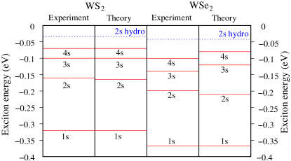
Figure 1: Excitonic spectrum: measurements and theory. The experimental data have been taken from Refs. Chernikov et al. (2014) and He et al. (2014) for WS₂ and WSe₂, respectively. The theoretical spectra have been calculated quasiclassically from Eq. (15) taking into account nonlocal screening and self-rotation. Our theory employs reduced exciton masses $\mu=0.16m_{0}$ for WS₂ and $\mu=0.17m_{0}$ for WSe₂ (here, $m_{0}$ is the free electron mass) computed ab initio in Ref. Berkelbach et al. (2013). We assume that the screening is due to the polarizability of the 2D layer $\chi=r_{0}/(2\pi)$ with $r_{0}$ being the only fitting parameter. In contrast to the conventional model Chernikov et al. (2014) strongly overestimating $r_{0}$, we found that $r_{0}=4.65$ nm for WS₂ and $r_{0}=3.84$ nm for WSe₂, in agreement with the ab initio calculations Berkelbach et al. (2013) suggesting $r_{0}\sim 4$ nm in such materials. Dotted lines show the first excited states ($2s$ states) within the standard hydrogenic model (6) to emphasize the qualitative difference with our findings.

Approach.— The two-body problem for Dirac particles is not trivial Sabio et al. (2010); Berman et al. (2013); Berkelbach et al. (2015); Wu et al. (2015); Berghäuser and Malic (2014); Stroucken and Koch (2015); De Martino and Egger (2017) because of the intrinsic coupling between conduction and valence band states making the electron and hole states entangled even without Coulomb interactions. We employ an effective exciton Hamiltonian that accounts for this coupling and has several advantages over that proposed in Ref. Rodin and Castro Neto (2013); see the Supplemental Material SM for details. The Hamiltonian can be written as $H=H_{0}+V(r)$, where $V(r)$ is the e-h interaction in relative coordinates, and $H_{0}$ is given by

$$H_{0}=\left(\begin{array}[]{cc}\frac{\hbar^{2}k^{2}}{2\mu}&\hbar k\sqrt{\frac{\Delta}{2\mu}}\mathrm{e}^{-i\theta}\\ \hbar k\sqrt{\frac{\Delta}{2\mu}}\mathrm{e}^{i\theta}&\Delta\end{array}\right).$$ (1)

Here, $\Delta$ is the band gap, $\mu$ is the exciton reduced mass, and $\tan\left(\theta\right)=k_{y}/k_{x}$. The spectrum of $H_{0}$ has two branches: a single parabolic branch $E_{k}=\Delta+\frac{\hbar^{2}k^{2}}{2\mu}$ describing excitonic states and, in contrast to Ref. Rodin and Castro Neto (2013), a dispersionless band $E_{0}=0$ being the vacuum state from which the excitons are initially excited. The corresponding eigenstates of $H_{0}$ can be written as $u_{k}=(\cos\left(\frac{\Phi}{2}\right),\sin\left(\frac{\Phi}{2}\right)\mathrm{e}^{i\theta})^{T}$ and $u_{0}=(\sin\left(\frac{\Phi}{2}\right),-\cos\left(\frac{\Phi}{2}\right)\mathrm{e}^{i\theta})^{T}$, where $\tan\left(\frac{\Phi}{2}\right)=\sqrt{\frac{2\mu\Delta}{\hbar^{2}k^{2}}}$. In order to make the model analytically tractable even for arbitrary $V(r)$ we rewrite $H$ in the quasiclassical form Zhou et al. (2015)

$$H_{\mathrm{exc}}=\Delta+\frac{\hbar^{2}k^{2}}{2\mu}+\frac{1}{2}\Omega\cdot(\nabla V\times k)+\frac{1}{4}\Omega\nabla^{2}V+V(r),$$ (2)

where $\Omega$ is the exciton Berry curvature Yao and Niu (2008); Garate and Franz (2011). The latter can be computed as Goerbig et al. (2014) $\Omega=\nabla_{k}\times\mathbf{A}$, with $\mathbf{A}$ being the Berry connection $\mathbf{A}=i\langle u_{k}|\nabla_{k}|u_{k}\rangle=-\sin^{2}\left(\frac{\Phi}{2}\right)\nabla_{k}\theta$. While the semiclassical expression (2) is general, the precise form of the quantum Hamiltonian (1) yields the particular Berry curvature $\Omega_{z}=\hbar^{2}\Delta/(\mu E_{k}^{2})\simeq\hbar^{2}/(\mu\Delta)$ that is twice the one-particle Berry curvature Xiao et al. (2007, 2012); Goerbig et al. (2014), in agreement with Ref. Zhou et al. (2015). The two-particle Berry curvature introduced here is a quantity describing the topology of an e-h pair, not of an electron and a hole separately. Since the potential $V(r)$ is circularly symmetric we employ cylindrical coordinates. To first order in $\partial_{r}V$, the total quasiclassical energy then reads

$$E_{\mathrm{tot}}=E_{k}+V(r)+\frac{\hbar^{2}\Delta}{2\mu rE_{k}^{2}}\frac{\partial V}{\partial r}\left(m+\frac{1}{2}\right),$$ (3)

where $m=0,\pm 1,\pm 2,...$ is the magnetic quantum number, and $E_{k}=\Delta+\frac{\hbar^{2}}{2\mu}\left(k_{r}^{2}+\frac{m^{2}}{r^{2}}\right)$. One notices that the last term is due to the Berry curvature that couples the quantum number $m$ and lifts the $m\leftrightarrow-m$ degeneracy as pointed out in Refs. Zhou et al. (2015); Srivastava and Imamogǧlu (2015). The $1/2$ offset is furthermore due to the Darwin-like term $\Omega\nabla^{2}V/4$ in Eq. (2), and one obtains the hydrogen model in the large-gap limit with $\Delta\rightarrow\infty$. Solving Eq. (3) with respect to the radial wave vector $k_{r}$, we then employ the Bohr-Sommerfeld quantization rule that in our case results in

$$\int\limits_{r_{1}}^{r_{2}}k_{r}dr=\pi\left(n+\frac{1}{2}\right),$$ (4)

where $n=0,1,2,...$ is the radial quantum number and $r_{1,2}$ are the quasiclassical turning points. Note that there are in general six solutions for $k_{r}$ but only one is real and positive. As we need only $s$-states to compare with experiments, we set $m=0$ everywhere from now on and consider a set of four models gradually approaching a simple but realistic one.

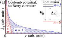
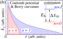
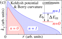
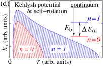
Figure 2: The plots show the phase space available for relative quasiclassical motion of a massive Dirac e-h pair in the ground and first excited $s$-states as well as the relative energy spacing between them. The relative spacing $\Delta E_{01}/E_{b}$ is proportional to the ratio between the two shaded areas. Parameters are taken to be relevant for WS₂. (a) Here, the Coulomb interaction with the effective dielectric constant $\epsilon=5.2$ adjusted to fit the binding energy measured Chernikov et al. (2014). Neither the dielectric constant nor the level spacing turn out to be compatible with the values measured. (b) The Coulomb-Berry model results in a reduced phase space ratio and, as a consequence, reduced relative level spacing between the $n=0$ and $n=1$ states. The effective dielectric constant taken to fit the binding energy is twice smaller than in (a). (c) Both Berry curvature and Keldysh potential are taken into account on the same footing. The relative level spacing (and the phase space ratio) is reduced even stronger, matching the measured spectrum at the screening radius of a few nm. (d) An approximate model where the Berry curvature is emulated by an internal angular momentum $j=1/2$ proving the concept of the self-rotating excitons in WS₂.

Coulomb model without Berry curvature.— This is the simplest exciton model possible, where the second term in Eq. (3) is neglected, and $V=-e^{2}/(\epsilon r)$. Equation (4) then explicitly reads

$$\int\limits_{r_{1}}^{r_{2}}dr\sqrt{\frac{2\mu}{\hbar^{2}}\left(E_{\mathrm{tot}}-\Delta+\frac{e^{2}}{\epsilon r}\right)}=\pi\left(n+\frac{1}{2}\right),$$ (5)

where $r_{1}=0$, as there is no tangential momentum, see Fig. 2(a), and $r_{2}=e^{2}/\epsilon(\Delta-E_{\mathrm{tot}})$. This results in the spectrum

$$E_{n}=\Delta-\frac{e^{4}\mu}{2\epsilon^{2}\hbar^{2}}\frac{1}{(n+1/2)^{2}},$$ (6)

where $n=0,1,2,...$ is the radial quantum number. In order order to fit the binding energy for WS₂ ($0.32$ eV Chernikov et al. (2014)) we have to take rather unrealistic effective dielectric constant $\epsilon=5.2$. Moreover, the level spacing remains heavily overestimated, see Fig. 1 and Fig. 2(a). These observations all together indicate that the standard exciton model is not suitable for 2DTMDs.

Coulomb-Berry model.— Here, we retain the Berry curvature in Eq. (3), which for the Coulomb interaction reads

$$E_{\mathrm{tot}}=\Delta+\frac{\hbar^{2}k_{r}^{2}}{2\mu}+\frac{e^{2}\hbar^{2}\Delta}{4\epsilon\mu r^{3}}\left(\Delta+\frac{\hbar^{2}k_{r}^{2}}{2\mu}\right)^{-2}-\frac{e^{2}}{\epsilon r}.$$ (7)

$E_{\mathrm{tot}}$ contains now a centrifugal-like term that makes the phase space near $r=0$ classically unavailable similar to what the conventional centrifugal term would do once $m\neq 0$. This is the most important intrinsic property of a self-rotating exciton that we believe to be crucial for a realistic model. Indeed, a real positive solution of Eq. (7) with respect to $\Delta+\frac{\hbar^{2}k_{r}^{2}}{2\mu}$ (and, hence, with respect to $k_{r}$) is only possible when

$$E_{\mathrm{tot}}+\frac{e^{2}}{\epsilon r}\geq\frac{3}{2r}\sqrt[3]{\frac{\hbar^{2}e^{2}\Delta}{2\epsilon\mu}}.$$ (8)

As consequence, the e-h distance $r$ cannot be smaller than $r_{1}$, where

$$r_{1}=\frac{1}{E_{\mathrm{tot}}}\left(\frac{3}{2}\sqrt[3]{\frac{e^{2}\hbar^{2}\Delta}{2\epsilon\mu}}-\frac{e^{2}}{\epsilon}\right).$$ (9)

Since $r_{1}$ must be positive we find that the effective Bohr radius $r_{B}=\epsilon\hbar^{2}/(\mu e^{2})$ must be larger than the effective Compton length $\lambda_{C}=\hbar/\sqrt{\mu\Delta}$. (The exact condition reads: $r_{B}>\lambda_{C}\sqrt{16/27}$.) The Compton length $\lambda_{C}$ has a similar meaning here as in high-energy physics: It constitutes the cutoff below which spontaneous particle creation and annihilation processes become important and the concept of an exciton as a two-particle system is no longer valid. From the band theory point of view, this corresponds to the critical regime when the exciton binding energy approaches the size of the band gap. The realistic parameters we employ in Fig. 1 and Table 1 suggest that both $\lambda_{C}$ and $r_{B}$ are a few angstrom that makes our excitons strongly nonhydrogenic even if the interaction is Coulomb-like.

Note that the Berry curvature is hidden not only in the integrand of Eq. (4) but in its limits as well. On the one hand, this makes an explicit solution rather cumbersome but possible. Indeed, Eq. (7) can be solved explicitly with respect to $k_{r}$ with the relevant branch given by

$$k_{r}=\sqrt{\frac{2\mu}{\hbar^{2}}\left(\frac{a}{3}+\frac{1+i\sqrt{3}}{6}c+\frac{2}{3}\frac{a^{2}}{(1+i\sqrt{3})c}-\Delta\right)},$$

where

$$c=\sqrt[3]{\frac{27b-2a^{3}-\sqrt{(27b-2a^{3})^{2}-4a^{6}}}{2}},$$

and $a=E_{\mathrm{tot}}+e^{2}/(\epsilon r)$, $b=(e^{2}\hbar^{2}\Delta)/(4\epsilon\mu r^{3})$. The lower limit is given by Eq. (9), whereas the upper limit can be approximately taken equal to $r_{2}$ given below Eq. (5). The latter is possible because the Berry term (being proportional to $1/r^{3}$) decreases much faster than the Coulomb potential at $r\to\infty$. On the other hand, the topological centrifugal effect occurs due to the pseudospin — the quantity associated with the $2\times 2$ matrix structure of the effective Hamiltonian (1). Similar to the real spin the pseudospin can be seen as an internal angular momentum of our exciton. The explicit diagonalization of our initial Hamiltonian $H$ has been performed in Ref. Trushin et al. (2016) within the shallow bound state approximation resulting in the $s$-states spectrum given by

$$E_{n}=\Delta-\frac{e^{4}\mu}{2\epsilon^{2}\hbar^{2}}\frac{1}{(n+|j|+1/2)^{2}},$$ (10)

where $j=1/2$ is the pseudospin quantum number. In Table 1 we compare the exciton energy spectra calculated from Eqs. (10) and (4) and find very good agreement for all excited states. The models do not agree on the ground state energy because of at least two reasons: (i) the quasiclassical approximation is unreliable at low energies, (ii) the shallow bound state condition $(\Delta-E_{n})/\Delta\ll 1$ may not be satisfied for $n=0$. The latter may indeed take place for WSe₂ where the band gap $\Delta=2.02$ eV He et al. (2014) is somewhat smaller than in WS₂ ($\Delta=2.41$ eV Chernikov et al. (2014)) hence resulting in a stronger discrepancy between the quasiclassical and quantum models.

$|E_{n}-\Delta|$, eV	$n=0$	$n=1$	$n=2$	$n=3$	$n=4$
WS2 (self-rot.)	0.320	0.080	0.035(5)	0.020	0.0128
WS2 (Berry)	0.315	0.081	0.036	0.020	0.013
WSe2 (self-rot.)	0.370	0.0925	0.041(1)	0.023	0.014
WSe2 (Berry)	0.344	0.0922	0.041	0.023	0.014

Table 1: The $j=1/2$ effective self-rotating exciton spectrum (10) is a good approximation for the quasiclassical Coulomb-Berry model introduced here. The dielectric constant is chosen to fit the binding energies $E_{b}$ measured in Refs. Chernikov et al. (2014) and He et al. (2014): $\epsilon=2.6$ ($E_{b}=0.32$ eV, $\Delta=2.41$ eV) for WS₂, and $\epsilon=2.5$ ($E_{b}=0.37$ eV, $\Delta=2.02$ eV) for WSe₂. The exciton reduced mass is the same as in Fig. 1.

Figure 2(b) shows how the Berry curvature reshapes the quasiclassically available phase space for the ground and lowest excited states. As compared to Fig. 2(a), the ratio between the two substantially decreases, hence, reducing the relative level spacing. If we again try to fit the binding energy for WS₂ by tuning the dielectric constant, we obtain the very reasonable number $\epsilon=2.52$ close to what one expects for graphene on SiO₂ substrate ($\epsilon_{\mathrm{SiO_{2}}}\sim 4$) with the upper surface exposed to air ($\epsilon_{\mathrm{Air}}\sim 1$) resulting in $\epsilon\sim 2.5$. However, the level spacing is not reduced strong enough to describe the exciton spectra on a quantitative level. To improve the predictive power of our approach we change the screening model.

Keldysh-Berry model.— Until now we have assumed that the dielectric function is local in real space, i.e., $q$ independent in reciprocal space. This is not true for 2D semiconducting systems, where the dielectric function is given by $\epsilon_{q}=1+2\pi\chi q$ Cudazzo et al. (2011); Latini et al. (2015); Olsen et al. (2016). The real-space e-h interaction potential is known as the Keldysh potential Keldysh (1979) given by

$$V(r)=-\frac{\pi e^{2}}{2r_{0}}\left[H_{0}\left(\frac{r}{r_{0}}\right)-Y_{0}\left(\frac{r}{r_{0}}\right)\right],$$ (11)

where $H_{0}$ is the Struve function, $Y_{0}$ is the Bessel function of the 2nd kind, and $r_{0}$ is the screening radius being the only fitting parameter. The Berry term in Eq. (3) contains now $\partial_{r}V$ given by

$$\frac{\partial V}{\partial r}=-\frac{\pi e^{2}}{2r_{0}^{2}}\left[Y_{1}\left(\frac{r}{r_{0}}\right)+H_{-1}\left(\frac{r}{r_{0}}\right)\right].$$ (12)

Because of the complexity of the $r$ dependence in Eqs. (11), (12), it is no longer possible to obtain explicit expressions for $r_{1,2}$ in Eq. (4), but we can write the condition for the existence of real values of $k_{r}$:

$$E_{\mathrm{tot}}-V(r)\geq\frac{3}{2}\sqrt[3]{\frac{\hbar^{2}\Delta}{2\mu r}\frac{\partial V}{\partial r}}.$$ (13)

One can see that this condition cannot be satisfied near $r=0$, which again confirms the quasiclassical inaccessibility of this region as if there were a nonzero tangential momentum. The available phase space can be qualitatively evaluated from Fig. 2(c). The ratio between phase spaces available for the ground and 1st excited states is further reduced making the level spacing even smaller than in the Coulomb-Berry model. The absolute value of binding energy measured in Refs. Chernikov et al. (2014); He et al. (2014) is matched at $r_{0}$ of a few nm compatible with ab initio calculations Berkelbach et al. (2013).

Self-rotating exciton model.— The Keldysh-Berry model while being realistic is too cumbersome for an express analysis of the experimental data. Aiming at a simplified model we employ the correspondence between the topological self-rotation and pseudospin angular momentum $j=1/2$; see Table 1. Generalizing this correspondence to any circularly symmetric potential, the quasiclassical energy for the excitonic $s$-states can be written as

$$E_{\mathrm{tot}}=\Delta+\frac{\hbar^{2}k_{r}^{2}}{2\mu}+\frac{\hbar^{2}j^{2}}{2\mu r^{2}}+V(r),$$ (14)

where $j=1/2$ is the the pseudospin angular momentum, and $V(r)$ is given by Eq. (11). The third term then mimics the Berry-curvature contribution and offers a good fit in the relevant intermediate-coupling regime, when $\alpha=e^{2}\sqrt{\mu/\Delta}/\hbar\epsilon\sim 1$ (or $\lambda_{C}$ approaches $r_{B}$). However, it becomes less accurate when $\Delta$ is drastically increased ($\alpha\ll 1$) and the Berry curvature vanishes as $1/\Delta$. In the opposite limit of decreasing $\Delta$ the self-rotating model becomes again inapplicable as soon as Eq. (13) cannot be satisfied for a certain $r>0$. This means that the system experiences an abrupt transition to a state that is no longer excitonic and that we do not aim to characterize here. The fitting model (14) does not describe this transition but matches the relevant physics once the system is already in a self-rotating regime, see the Supplemental Material SM for details.

The quantization condition with the effective $j=1/2$ self-rotation reads

$$\int\limits_{r_{1}}^{r_{2}}dr\sqrt{\frac{2\mu}{\hbar^{2}}\left[E_{\mathrm{tot}}-\Delta-V(r)\right]-\frac{j^{2}}{r^{2}}}=\pi\left(n+\frac{1}{2}\right),$$ (15)

where $r_{1,2}$ are determined by imposing the zero condition on the integrand. The qualitative justification of this model follows from Fig. 2(d): the quasiclassically available phase space appears to be very close to the one obtained within a somewhat more accurate approach depicted in Fig. 2(c). The major merit of the $j=1/2$ effective model is its transparency in describing the self-rotation and non-Coulomb potential on the equal footing. It can easily be employed to fit the exciton spectra in Dirac materials Wehling et al. (2014) once they will be measured in future.

We use Eq. (15) to compute the energy for a given $n$; see Fig. 1. The model perfectly fits the exciton spectrum measured in WS₂ employing $r_{0}\sim 4$ nm, as predicted ab initio in Berkelbach et al. (2013). The agreement is less good in the case of WSe₂. This may be due to a certain incompatibility between the experimental data Chernikov et al. (2014); He et al. (2014) and ab initio predictions Berkelbach et al. (2013): The exciton binding energy measured in WSe₂ turns out to be higher than in WS₂, whereas the ab initio theory Berkelbach et al. (2013) predicts an opposite trend. Once the band gap $\Delta=2.02$ eV (and, hence, the binding energy $E_{b}=0.37$ eV) is reduced by a few tens of meV the exciton spectrum can be fitted for WSe₂ as good as for WS₂. However, we emphasize that our model fits the data anyway much better than the conventional exciton model without Berry curvature.

Conclusion.— The very fact that the exciton spectrum in 2DTMDs Chernikov et al. (2014); He et al. (2014); Hill et al. (2015) does not resemble the conventional Rydberg series has been discussed in multiple papers recently Olsen et al. (2016); Berkelbach et al. (2015); Wu et al. (2015); Berghäuser and Malic (2014); Stroucken and Koch (2015); Zhou et al. (2015); Srivastava and Imamogǧlu (2015); Trushin et al. (2017); Ye et al. (2014); Qiu et al. (2013); Ramasubramaniam (2012); Komsa and Krasheninnikov (2012); Shi et al. (2013); Cheiwchanchamnangij and Lambrecht (2012); Echeverry et al. (2016); Wang et al. (2015). The commonly-accepted explanation Chernikov et al. (2014) in terms of the nonlocal screening of the bare Coulomb potential Cudazzo et al. (2011) fits well the exciton spectrum measured Chernikov et al. (2014) as long as an unrealistically high 2D polarizability is assumed. To cure this inconsistency, contributions from the Berry curvature need to be considered. The Berry curvature provides a strong repulsion when $r\rightarrow 0$ even for $s$-states with no angular momentum. We have shown that this repulsion can be accounted for in a model where the excitons in 2DTMDs are self-rotating in a way similar to the quasiparticles on the surface of a strong topological insulator Garate and Franz (2011), thus opening further perspectives for excitonic engineering in van der Waals heterostructures Wu et al. (2017).

We acknowledge financial support from the Center of Applied Photonics funded by the DFG-Excellence Initiative. M.T. was supported by the Director’s Senior Research Fellowship from the Centre for Advanced 2D Materials at the National University of Singapore (NRF Medium Sized Centre Programme R-723-000-001-281). We thank Alexey Chernikov and Oleg Berman for discussions.

Appendix A Effective exciton Hamiltonian

Here, we justify the effective excitonic Hamiltonian suggested in the main text. We focus on the $K$-valley, where free electrons (e) are described by the two-dimensional Dirac Hamiltonian given by

$$H_{e}=\left(\begin{array}[]{cc}M&\hbar vke^{-i\theta}\\ \hbar vke^{i\theta}&-M\\ \end{array}\right),\quad$$ (16)

where $\tan\theta=k_{y}/k_{x}$, and $\Delta=2M$ is the fundamental band gap. The corresponding free hole (h) Hamiltonian $H_{h}$ at zero center-of-mass momentum reads Rodin and Castro Neto (2013)

$$H_{h}=\left(\begin{array}[]{cc}-M&\hbar vke^{i\theta}\\ \hbar vke^{-i\theta}&M\\ \end{array}\right).$$ (17)

Here, we have assumed that the electron and hole have opposite momenta for optical excitons we consider. The angle $\theta$ has therefore been changed to $\theta+\pi$ for holes. This has been done in Rodin and Castro Neto (2013) at a later stage.

These two Hamiltonians suggest the same quasiparticle dispersion

$$\varepsilon_{k}=\sqrt{(\hbar vk)^{2}+M^{2}},$$ (18)

that in turn suggests the same effective mass $m^{*}=M/v^{2}=\Delta/(2v^{2})$ for both e and h. The kinetic term for the minimal exciton model with zero center-of-mass momentum should therefore read as $\hbar^{2}k^{2}/(2\mu)$, where $\mu=m_{e}m_{h}/(m_{e}+m_{h})=m^{*}/2=M/(2v^{2})=\Delta/(4v^{2})$ is the reduced effective mass. This model, however, does not take into account the pseudospin degree of freedom that makes the electron and hole states entangled even without Coulomb interaction.

The correct two-particle e-h Hamiltonian with vanishing interaction is given by the Kronecker sum $H_{4}=H_{e}\otimes I_{2}+I_{2}\otimes H_{h}$ with $I_{2}$ being the $2\times 2$ unit matrix. Since the one-particle electron Hamiltonian $H_{e}$ already has an electron and a hole branch, one might not see the ”need” to extend the dimension of our Hilbert space. However, this is a flaw since electron and hole branches are intimately related on the single-particle level in Dirac-like Hamiltonians such that they do not represent two different particles. That is why the two-body problem consists of a tensor product of two Dirac particles, each of which has its own electron and hole branch. Hence, we have Rodin and Castro Neto (2013)

$$H_{4}=\left(\begin{array}[]{cccc}0&e^{i\theta}\hbar kv&e^{-i\theta}\hbar kv&0\\ e^{-i\theta}\hbar kv&2M&0&e^{-i\theta}\hbar kv\\ e^{i\theta}\hbar kv&0&-2M&e^{i\theta}\hbar kv\\ 0&e^{i\theta}\hbar kv&e^{-i\theta}\hbar kv&0\\ \end{array}\right).$$ (19)

The Hamiltonian $H_{4}$ has four eigenvalues:

$$\left\{0,0,+2\sqrt{\hbar^{2}v^{2}k^{2}+M^{2}},-2\sqrt{\hbar^{2}v^{2}k^{2}+M^{2}}\right\}.$$

The physical meaning of the four states can be analyzed having two excited particles in play. The exciton state corresponds to an electron in the conduction band and a hole in the valence band. One of two zero-energy states corresponds to the exciton vacuum when all the holes are in the conduction band and all the electrons are in the valence band. The second zero-energy state corresponds to the inverse population (inverted vacuum) when all the electrons are in the conduction band and all the holes are in the valence band. Finally, the negative-dispersion branch corresponds to a single electron in the valence band and a single hole in the conduction band that is an exciton created in the inverted vacuum. Obviously, the latter two configurations are not relevant for our setting with the low-intensity optical excitations. Thus, we extract the excitonic part out of the Hamiltonian $H_{4}$. This is done in two steps. First, we extract the relevant $2\times 2$ block via an appropriate unitary transformation. This block contains the positive excitonic band plus a zero-energy flat band. While we are interested, from a purely spectral point of view, only in the positive branch, the coupling to the zero-energy band bears relevant information about the Berry-curvature contributions that we discuss in more detail in the following section. In a second step, we consider the $2\times 2$ block up to second order in momentum. Its Dirac-type structure allows us to calculate directly the Berry curvature of the exciton branch. The consistency of its expression with that of a quasiclassical approach corroborates the validity of the effective quantum Hamiltonian obtained within our work.

In detail, to transform $H_{4}$ into the block-diagonal form, we use the transformation matrix

$$P=\left(\begin{array}[]{cccc}\cos\left(\frac{\Theta}{2}\right)&0&\sin\left(\frac{\Theta}{2}\right)&0\\ 0&\cos\left(\frac{\Theta}{2}\right)&0&\sin\left(\frac{\Theta}{2}\right)\\ e^{i\theta}\sin\left(\frac{\Theta}{2}\right)&0&-e^{i\theta}\cos\left(\frac{\Theta}{2}\right)&0\\ 0&e^{i\theta}\sin\left(\frac{\Theta}{2}\right)&0&-e^{i\theta}\cos\left(\frac{\Theta}{2}\right)\\ \end{array}\right),$$ (20)

where

$$\tan\Theta=\frac{\hbar vk}{M}.$$

The transformed matrix $H_{4}^{\prime}=P^{-1}H_{4}P$ then reads

$$H_{4}^{\prime}=\left(\begin{array}[]{cccc}-M+\varepsilon_{k}&e^{i\theta}\hbar kv&0&0\\ e^{-i\theta}\hbar kv&M+\varepsilon_{k}&0&0\\ 0&0&-M-\varepsilon_{k}&e^{i\theta}\hbar kv\\ 0&0&e^{-i\theta}\hbar kv&M-\varepsilon_{k}\\ \end{array}\right),\\$$ (21)

where $\varepsilon_{k}$ is given by equation (18). The upper left block $2\times 2$ has two eigenvalues $\left\{0,+2\sqrt{\hbar^{2}v^{2}k^{2}+M^{2}}\right\}$ describing excitonic quasiparticles we are interested in. The block is decoupled from the rest and can be seen as a reduced excitonic Hamiltonian:

$$H_{2}=\left(\begin{array}[]{cc}-M+\sqrt{\hbar^{2}v^{2}k^{2}+M^{2}}&e^{i\theta}\hbar kv\\ e^{-i\theta}\hbar kv&M+\sqrt{\hbar^{2}v^{2}k^{2}+M^{2}}\\ \end{array}\right).$$ (22)

Note that the dispersion $2\sqrt{\hbar^{2}v^{2}k^{2}+M^{2}}$ once written in the effective mass approximation suggests correct reduced mass $\mu=M/(2v^{2})=\Delta/(4v^{2})$. Once the Schrödinger terms are neglected and the missing momentum is compensated by the factor of 2 in the off-diagonal terms we obtain the reduced excitonic Hamiltonian given by

$$H_{2}^{\mathrm{RCN}}=\left(\begin{array}[]{cc}M&2\hbar kve^{i\theta}\\ 2\hbar kve^{-i\theta}&-M\\ \end{array}\right).$$ (23)

This form has been suggested by Rodin and Castro Neto in Ref. Rodin and Castro Neto (2013) but it has two major drawbacks:

• Its spectrum $\pm\sqrt{(2\hbar vk)^{2}+M^{2}}$ suggests the effective reduced mass $M/4v^{2}$ twice smaller than needed ($M/2v^{2}$). As a consequence, the excitonic Berry curvature would read $\Omega^{\mathrm{RCN}}_{\mathrm{exc}}(k=0)=2\hbar^{2}v^{2}/M^{2}=8\hbar^{2}v^{2}/\Delta^{2}$, which is twice as large as the one obtained by Zhou et al. Zhou et al. (2015).

• The lower dispersionless branch describing zero-energy states is substituted by an “antiparticle” branch that contradicts to physical meaning of the vacuum state from which the excitons are excited.

To remedy the situation we must retain both Dirac and Schrödinger terms in equation (22). At the same time, the Hamiltonian must be parametrized in such a way that the lower spectral branch always remains dispersionless. The dispersionless vacuum state is of utmost importance for optically excited excitons where electron and hole momenta are antiparallel and, hence, cancel each other once an exciton recombines. Any vacuum state with dispersion suggests some uncompensated momentum and violates momentum conservation for direct-gap optical excitons.

We aim for an exciton model in terms of the effective mass, so that we consider the case of small $k$ and expand the energy of e-h relative motion up to the terms quadratic in $k$. If we keep quadratic terms in both lines of the matrix (22), then we end up with the spectrum quartic in $k$. To avoid this inconvenience we expand each element of the matrix up to the lowest non-zero order as follows:

$$-M+\sqrt{\hbar^{2}v^{2}k^{2}+M^{2}}\propto k^{2},\quad M+\sqrt{\hbar^{2}v^{2}k^{2}+M^{2}}\to 2M.$$

Then, we modify the Dirac part in order to compensate parasitic terms in the dispersionless branch arising due to the different approximations done in these two terms, and $H_{2}$ reads

$$H_{2}^{\mathrm{eff}}=\left(\begin{array}[]{cc}\frac{\hbar^{2}v^{2}k^{2}}{M}&e^{i\theta}\sqrt{2}\hbar vk\\ e^{-i\theta}\sqrt{2}\hbar vk&2M\\ \end{array}\right).$$ (24)

Despite different approximations done in lower and upper lines of equation (24) the Hamiltonian obtained satisfies all physical criteria we demand:

• $H_{2}^{\mathrm{eff}}$ results in two spectral branches, $E_{0}=0$ and $E_{k}=2M+\frac{\hbar^{2}v^{2}k^{2}}{M}$, where the latter suggests correct reduced mass, $\mu=M/2v^{2}$.

• The vacuum state remains dispersionless, as it is expected from the correct excitonic Hamiltonian (22) and physical constrains explained above.

• The two spectral branches remain entangled, as it is again expected for Dirac excitons.

• The Hamiltonian contains the Schrödinger term that preserves the exciton from a collapse.

Equation (24) can be rewritten in terms of the reduced effective mass $\mu=M/2v^{2}$ as

$$H_{2}^{\mathrm{eff}}=\left(\begin{array}[]{cc}\frac{\hbar^{2}k^{2}}{2\mu}&e^{i\theta}\hbar k\sqrt{\frac{M}{\mu}}\\ e^{-i\theta}\hbar k\sqrt{\frac{M}{\mu}}&2M\\ \end{array}\right).$$ (25)

We use this version in our quasiclassical model as an effective exciton Hamiltonian with vanishing interaction. It is clear that, once $\mu$ is fixed, there is only one possible form of $H_{2}^{\mathrm{eff}}$ providing a dispersionless branch for the vacuum state. One can easily obtain the Berry curvature of the exciton band, which is written at $k=0$ as

$$\Omega_{\mathrm{exc}}^{\mathrm{eff}}(k=0)=\frac{\hbar^{2}}{\mu\Delta}=2\frac{\hbar^{2}}{m^{*}\Delta}=2\Omega_{e}(k=0),$$ (26)

i.e. it is twice the electronic Berry curvature $\Omega_{e}(k=0)=\hbar^{2}/m^{*}\Delta$ derived form $H_{e}$, see equation (16). This agrees with the quasiclassical analysis of Ref. Zhou et al. (2015), where the exciton Berry curvature was shown to be $\Omega_{\mathrm{exc}}(k=0)=\Omega_{e}(k=0)-\Omega_{h}(k=0)$, in terms of the Berry curvature of the one-particle Dirac models (16) and (17), for the electron and the hole, respectively. Since in this case, one has $\Omega_{e}(k)=-\Omega_{h}(k)$, one obtains $\Omega_{\mathrm{exc}}(k=0)=2\Omega_{e}(k=0)$, in agreement with the Berry curvature obtained from our effective $2\times 2$ Hamiltonian (25).

Appendix B Semi-quantitative justification for the self-rotating exciton model in the intermediate coupling regime

We now use the semi-classical exciton Hamiltonian derived in Ref. Zhou et al. (2015) taking into account the Berry curvature,

$${H}_{\mathrm{exc}} = \Delta+\frac{{\bf p}}{2\mu}+{V}(r)$$

$$+\frac{1}{2\hbar}\Omega({\bf p})\cdot\left[\frac{\partial{V}(r)}{\partial\mathbf{r}}\times{\bf p}\right]+\frac{1}{4}\Omega({\bf p})\nabla^{2}{V}(r),$$

in terms of the relative coordinate $\mathbf{r}$ and momentum ${\bf p}=\hbar{\bf k}$ of the exciton, and use

$$\Omega_{z}({\bf p}=0)\equiv\Omega_{\mathrm{exc}}^{\mathrm{eff}}(k=0)$$ (28)

for the Berry curvature, see equation (26). We furthermore introduce the “Compton length” $\lambda_{C}=\hbar/\sqrt{\Delta\mu}$, which constitutes one of the natural length scales of the problem (it could also be called the gap length here) and that we will use in the expression of the Hamiltonian, which reads (in cylinder coordinates)

$${H}_{\mathrm{exc}} = \Delta\left[1+\frac{\lambda_{C}^{2}}{2}\left({k}_{r}^{2}+\frac{m^{2}}{r^{2}}\right)\right]$$ (29)

$$+{V}(r)+\frac{\lambda_{C}^{2}}{2r}\frac{\partial{V}}{\partial r}\left(m+\frac{1}{2}\right),$$

where $m=0,\pm 1,\pm 2,...$ is the quantum number of the tangential momentum, and $k_{r}$ is the radial wave-vector. If we now consider a Coulomb interaction ${V}(r)=-e^{2}/\epsilon r=-\alpha\Delta(\lambda_{C}/r)$, in terms of the dimensionless coupling strength $\alpha=(e^{2}/\hbar\epsilon)\sqrt{\mu/\Delta}$, one can write down the Hamiltonian in a dimensionless manner

$$\frac{{H}_{\mathrm{exc}}}{\Delta} = 1+\frac{1}{2}\left(\lambda_{C}^{2}k_{r}^{2}+m^{2}\frac{\lambda_{C}^{2}}{r^{2}}\right)$$ (30)

$$-\alpha\frac{\lambda_{C}}{r}+\frac{\alpha}{2}\left(m+\frac{1}{2}\right)\left(\frac{\lambda_{C}}{r}\right)^{3}.$$

Notice that one could also have chosen the Bohr radius $r_{B}=\hbar^{2}\epsilon/\mu e^{2}$ as a natural length scale. This choice is mostly made in the context of the 2D hydrogen model. It is related to the Compton length by $\lambda_{C}=\alpha r_{B}$ – a third length scale is given by the comparison between interaction and gap, $\ell=e^{2}/\epsilon\Delta$, and one finds the hierarchy

$$\ell=\alpha\lambda_{C}=\alpha^{2}r_{B}.$$ (31)

The Compton length has a similar meaning here as in high-energy physics. It constitutes the lower bound of the length scale above which the exciton problem can be treated in terms of relativistic quantum mechanics, such as in our present approach. On length scales lower than $\lambda_{C}$, one needs to take into account spontaneous electron-hole creation processes that could eventually provide (on the average) additional screening to the effective interaction potential ${V}(r)$. For $\alpha\lesssim 1$, the Bohr radius is indeed larger than $\lambda_{C}$, and the above-mentioned processes can be safely neglected. This argument in terms of length scales is in line with one obtained from energy scales: in order to be allowed to restrict the exciton dynamics to a single band (i.e. an electron in the conduction and a hole in the valence band), one needs to ensure that the exciton energy $\sim e^{2}/\epsilon r_{B}$ (for a typical exciton size given by the Bohr radius, as for the $s$ state) is small as compared to the gap $\Delta$, but the ratio is precisely given by $e^{2}/\epsilon r_{B}\Delta=\ell/r_{B}=\alpha^{2}$, such that one obtains again $\alpha\lesssim 1$.

While the above expression (30) is well adapted to connect the problem to the non-interacting case, by setting $\alpha\rightarrow 0$, it does not really allow us to appreciate the relative role of the two interaction terms. In units of $r_{B}$, the Hamiltonian then reads

$$\frac{{H}_{\mathrm{exc}}}{\Delta} = 1+\frac{\alpha^{2}}{2}\left(r_{B}^{2}k_{r}^{2}+m^{2}\frac{r_{B}^{2}}{r^{2}}\right)$$ (32)

$$-\alpha^{2}\frac{r_{B}}{r}+\frac{\alpha^{4}}{2}\left(m+\frac{1}{2}\right)\left(\frac{r_{B}}{r}\right)^{3},$$

and one now realizes that in the weak-coupling limit ($\alpha\ll 1$), where the typical length scale is indeed set by the Bohr radius, one retrieves the 2D hydrogen problem since the Berry-curvature term becomes less relevant ($\alpha^{4}$ instead of the leading $\alpha^{2}$). This may be seen as a consistency test of the quasiclassical treatment since one expects indeed to retrieve the hydrogen problem, described in terms of a simple one-band Schrödinger equation, in this limit. In our case (2D transition-metal dichalcogenides), however, we are in an intermediate-coupling regime, with $\Delta\sim 2$ eV and $m_{e}\simeq m_{h}\simeq 0.1m_{0}$ ($m_{0}$ is the bare electron mass) suggesting $\alpha\simeq(2...3)/\epsilon$, that is on the order of unity for a typical dielectric constant of $\epsilon\simeq 2.5$.

From the above discussion we see that the self-rotating model is a good description in this limit of intermediate couplings. Naturally, the Berry-curvature term scales as $(r_{B}/r)^{3}$, thus prohibiting strictu sensu a description in terms of a centrifugal term that scales as $(r_{B}/r)^{2}$. However, the typical exciton radius in the $s$ (and even $p$) states is on the order of $r_{B}$, for principal quantum numbers that are not too large. In this case, one might try to merge the Berry-curvature and the centrifugal term in a rather crude manner,

$$m^{2}+\alpha^{2}m+\alpha^{2}/2\simeq j^{2}+c,$$ (33)

where $j=(m+\alpha^{2}/2)$ and we have introduced a corrective term (the error one makes in absorbing the Berry-curvature term in a $j^{2}$), $c=\alpha^{2}/2-\alpha^{4}/4$. While this corrective term vanishes for $\alpha=\sqrt{2}$, it is $1/4$ for $\alpha=1$ that yields $j=m+1/2$ as stipulated within the self-rotating model.

While our analysis shows that the self-rotating approximation is indeed a good one for values of $\alpha\sim 1$, it breaks down in the weak-coupling limit, where one retrieves the hydrogen problem. Furthermore, it might also be inappropriate in the discussion of large values of $m$ (and $n$) where the effective radius (i.e. the extension of the wave function) is substantially larger than $r_{B}$. From a theoretical point of view, it might therefore be reasonable to compare the different models (just Coulomb for the moment) in these large-$m$ and large-$n$ limits even if this limit does not seem relevant in the physical properties of excitons in 2D transition-metal dichalcogenides on the experimental side. This would allow us to test the limits of the self-rotating approximation for $\alpha\sim 1$.

References

- Elliott (1957) R. J. Elliott, Phys. Rev. 108, 1384 (1957).
- Xiao et al. (2012) D. Xiao, G.-B. Liu, W. Feng, X. Xu, and W. Yao, Phys. Rev. Lett. 108, 196802 (2012).
- Zhou et al. (2015) J. Zhou, W.-Y. Shan, W. Yao, and D. Xiao, Phys. Rev. Lett. 115, 166803 (2015).
- Srivastava and Imamogǧlu (2015) A. Srivastava and A. Imamogǧlu, Phys. Rev. Lett. 115, 166802 (2015).
- Gong et al. (2017a) P. Gong, H. Yu, Y. Wang, and W. Yao, Phys. Rev. B 95, 125420 (2017a).
- Gong et al. (2017b) Z. R. Gong, W. Z. Luo, Z. F. Jiang, and H. C. Fu, Sci. Rep. 7, 42390 (2017b).
- Keldysh (1979) L. V. Keldysh, Pis’ma Zh. Eksp. Teor. Fiz. 29, 716 (1979).
- Cudazzo et al. (2011) P. Cudazzo, I. V. Tokatly, and A. Rubio, Phys. Rev. B 84, 085406 (2011).
- Chernikov et al. (2014) A. Chernikov, T. C. Berkelbach, H. M. Hill, A. Rigosi, Y. Li, O. B. Aslan, D. R. Reichman, M. S. Hybertsen, and T. F. Heinz, Phys. Rev. Lett. 113, 076802 (2014).
- He et al. (2014) K. He, N. Kumar, L. Zhao, Z. Wang, K. F. Mak, H. Zhao, and J. Shan, Phys. Rev. Lett. 113, 026803 (2014).
- Berkelbach et al. (2013) T. C. Berkelbach, M. S. Hybertsen, and D. R. Reichman, Phys. Rev. B 88, 045318 (2013).
- Sabio et al. (2010) J. Sabio, F. Sols, and F. Guinea, Phys. Rev. B 81, 045428 (2010).
- Berman et al. (2013) O. L. Berman, R. Y. Kezerashvili, and K. Ziegler, Phys. Rev. A 87, 042513 (2013).
- Berkelbach et al. (2015) T. C. Berkelbach, M. S. Hybertsen, and D. R. Reichman, Phys. Rev. B 92, 085413 (2015).
- Wu et al. (2015) F. Wu, F. Qu, and A. H. MacDonald, Phys. Rev. B 91, 075310 (2015).
- Berghäuser and Malic (2014) G. Berghäuser and E. Malic, Phys. Rev. B 89, 125309 (2014).
- Stroucken and Koch (2015) T. Stroucken and S. W. Koch, J. Phys. Condensed Matter 27, 345003 (2015).
- De Martino and Egger (2017) A. De Martino and R. Egger, Phys. Rev. B 95, 085418 (2017).
- Rodin and Castro Neto (2013) A. S. Rodin and A. H. Castro Neto, Phys. Rev. B 88, 195437 (2013).
- (20) Supplemental Material is included as an Appendix in this submission.
- Yao and Niu (2008) W. Yao and Q. Niu, Phys. Rev. Lett. 101, 106401 (2008).
- Garate and Franz (2011) I. Garate and M. Franz, Phys. Rev. B 84, 045403 (2011).
- Goerbig et al. (2014) M. O. Goerbig, G. Montambaux, and F. Piéchon, Europhys. Lett. 105, 57005 (2014).
- Xiao et al. (2007) D. Xiao, W. Yao, and Q. Niu, Phys. Rev. Lett. 99, 236809 (2007).
- Trushin et al. (2016) M. Trushin, M. O. Goerbig, and W. Belzig, Phys. Rev. B 94, 041301 (2016).
- Latini et al. (2015) S. Latini, T. Olsen, and K. S. Thygesen, Phys. Rev. B 92, 245123 (2015).
- Olsen et al. (2016) T. Olsen, S. Latini, F. Rasmussen, and K. S. Thygesen, Phys. Rev. Lett. 116, 056401 (2016).
- Wehling et al. (2014) T. Wehling, A. Black-Schaffer, and A. Balatsky, Adv. Phys. 63, 1 (2014).
- Hill et al. (2015) H. M. Hill, A. F. Rigosi, C. Roquelet, A. Chernikov, T. C. Berkelbach, D. R. Reichman, M. S. Hybertsen, L. E. Brus, and T. F. Heinz, Nano Lett. 15, 2992 (2015).
- Trushin et al. (2017) M. Trushin, M. O. Goerbig, and W. Belzig, J. Phys. Conf. Series 864, 012033 (2017).
- Ye et al. (2014) Z. Ye, T. Cao, K. O’Brien, H. Zhu, X. Yin, Y. Wang, S. G. Louie, and X. Zhang, Nature (London) 513, 214 (2014).
- Qiu et al. (2013) D. Y. Qiu, F. H. da Jornada, and S. G. Louie, Phys. Rev. Lett. 111, 216805 (2013).
- Ramasubramaniam (2012) A. Ramasubramaniam, Phys. Rev. B 86, 115409 (2012).
- Komsa and Krasheninnikov (2012) H.-P. Komsa and A. V. Krasheninnikov, Phys. Rev. B 86, 241201 (2012).
- Shi et al. (2013) H. Shi, H. Pan, Y.-W. Zhang, and B. I. Yakobson, Phys. Rev. B 87, 155304 (2013).
- Cheiwchanchamnangij and Lambrecht (2012) T. Cheiwchanchamnangij and W. R. L. Lambrecht, Phys. Rev. B 85, 205302 (2012).
- Echeverry et al. (2016) J. P. Echeverry, B. Urbaszek, T. Amand, X. Marie, and I. C. Gerber, Phys. Rev. B 93, 121107 (2016).
- Wang et al. (2015) G. Wang, I. C. Gerber, L. Bouet, D. Lagarde, A. Balocchi, M. Vidal, T. Amand, X. Marie, and B. Urbaszek, 2D Materials 2, 045005 (2015).
- Wu et al. (2017) F. Wu, T. Lovorn, and A. H. MacDonald, Phys. Rev. Lett. 118, 147401 (2017).