JDFTx: software for joint density-functional theory

Abstract

Density-functional theory (DFT) has revolutionized computational prediction of atomic-scale properties from first principles in physics, chemistry and materials science. Continuing development of new methods is necessary for accurate predictions of new classes of materials and properties, and for connecting to nano- and mesoscale properties using coarse-grained theories. JDFTx is a fully-featured open-source electronic DFT software designed specifically to facilitate rapid development of new theories, models and algorithms. Using an algebraic formulation as an abstraction layer, compact C++11 code automatically performs well on diverse hardware including GPUs (Graphics Processing Units). This code hosts the development of joint density-functional theory (JDFT) that combines electronic DFT with classical DFT and continuum models of liquids for first-principles calculations of solvated and electrochemical systems. In addition, the modular nature of the code makes it easy to extend and interface with, facilitating the development of multi-scale toolkits that connect to ab initio calculations, e.g. photo-excited carrier dynamics combining electron and phonon calculations with electromagnetic simulations.

1 Motivation and significance

Density functional theory (DFT) enables computational prediction of material properties and chemical reactions starting from a quantum mechanical description of the electrons. DFT codes are now widely used to understand and design new materials from first principles through the prediction of electronic properties, structures and dynamics of molecules, solids and surfaces. Such studies commonly employ proprietary software such as GAUSSIAN [1] and VASP [2] as well as open-source software such as Quantum Espresso [3], ABINIT [4] and Qbox [5], to name just a few.

However, DFT offers limited accuracy for certain classes of materials and properties [6], and is extremely computationally expensive for amorphous materials, liquids and nanostructures [7]. The study of new systems, as soon as they become technologically and scientifically relevant, requires continual development of new methods to improve the accuracy of DFT and incorporate it into multi-scale theories to access higher length scales. Developing and testing such methods within production codes is extremely challenging and time consuming.

Systems involving liquids, such as electrochemical interfaces or solvated biomolecules, are particularly challenging for DFT calculations, requiring thermodynamic sampling of several thousands of atomic configurations in ab initio molecular dynamics (AIMD) simulations [8]. Joint density-functional theory (JDFT) was proposed as a theoretical framework to address this issue by combining electronic DFT with classical DFT of liquids [9] to directly compute equilibrium properties of quantum-mechanically described solutes in diverse solvent environments [10]. Bringing this method to fruition required the simultaneous development of physical models (free energy functionals) of liquids and their interaction with electrons, algorithms to perform variational free-energy minimization and code that tightly and efficiently coupled these new models with electronic DFT. We began the open-source software project JDFTx in 2012 to facilitate this combined model, algorithm and code development effort.

Listing 1: JDFTx code for a simplified solvation model with local dielectric screening. The extended DFT++ algebraic formulation [11, 12] expresses the physical model in almost the same language as the defining equations (1) and (2), while parallel implementations of the operators make this code, written only once, run with multiple CPU threads (using pthreads) or on NVIDIA GPUs (using CUDA).

⬇

class LinearPCM : public LinearSolvable<ScalarFieldTilde>

{ ScalarField epsilon; //inhomogeneous dielectric

public:

virtual ScalarFieldTilde hessian(const ScalarFieldTilde& phiTilde) const

{ return (-1./(4*M_PI)) * divergence(J(epsilon * I(gradient(phiTilde))));

}

double getAdiel(const ScalarFieldTilde& rhoTilde) const

{ solve(rhoTilde); //solve hessian(state) = rhoTilde

return 0.5 * dot(state - coulomb(rhoTilde), O(rhoTilde));

}

};

This article introduces JDFTx as a general-purpose user-friendly DFT software that offers a full feature set, yet is simultaneously developer-friendly to enable rapid prototyping of new electronic-structure and related methods. Section 2 presents the overall design of JDFTx using the algebraic formulation of DFT [11, 12] to separate implementation into physics, algorithm and hardware layers, enabling rapid development of high-performance code that is easy to use. It also outlines commonly used features of the code, some of which are illustrated in more detail with examples in section 3. Finally, section 4 highlights new methods that have already been developed using JDFTx, including a hierarchy of JDFT models for the electronic structure of solvated systems and a toolkit for photo-excited carrier dynamics with ab initio electron and phonon properties, as well as key applications of these methods.

2 Software description

The core functionality of any electronic DFT software includes the calculation of ground-state electron densities, energies and forces within the Kohn-Sham DFT formalism [13], given a list of atoms and their positions. This facilitates prediction of structure and dynamics of materials, evaluation of reaction pathways and chemical kinetics, as well as determination of phase equilibria and stability.

Due to the nature of quantum-mechanical simulations of matter, DFT calculations become increasingly expensive with the number of atoms and electrons involved; computational complexity ranges from $O(N^{3})$ (with a smaller prefactor) to $O(N)$ (with a much larger prefactor), depending on the implementation. A brute force approach to nano and mesoscale systems with several thousands to millions of atoms is therefore not practical; it is instead logical to develop multi-scale theories for the properties of interest while still incorporating DFT electronic structure where appropriate.

JDFTx is an open-source DFT software designed specifically with the goals of coupling electronic DFT with coarse-grained theories to bridge atomic and system length scales, and of facilitating the rapid development of new classes of such combined theories. It implements electronic DFT in the plane-wave basis, which is best suited for periodic systems such as solids and solid surfaces, but is also applicable to molecular systems. A key functionality of JDFTx beyond standard electronic DFT codes is the modeling of liquids using classical DFT [12], and JDFT calculations of electronic structure in liquid environments by combining electronic DFT with classical DFT or simpler solvation models. Section 2.1 presents a birds-eye view of the code architecture along with a code example to illustrate the ease of developing new features, after which section 2.2 outlines the key features of the code.

Figure 1: Organization of the JDFTx code: key classes/files shown in black, organized into sub-directories shown in green and compilation targets (executables/libraries) shown in red. $A\bullet---B$ indicates $A$ contains $B$, while $A{\color[rgb]{0,0,0.7}\definecolor[named]{pgfstrokecolor}{rgb}{0,0,0.7}\longleftarrow}B$ indicates $A$ inherits from $B$. Lightweight executables jdftx, phonon and wannier link to a dynamic link library, libjdftx, which contains most of the functionality and can be readily used from third-party codes. With CUDA available, compilation of the same code additionally results in jdftx_gpu, phonon_gpu etc. that run almost entirely on compute-capable GPUs. Only a small fraction of files and connections are shown here; see the API documentation at %****␣submit.tex␣Line␣200␣****http://jdftx.org for more details.

2.1 Software Architecture

JDFTx achieves its goal of code simplicity and extensibility by using the ‘DFT++’ algebraic formulation of electronic DFT [11] and its generalization to classical DFT and JDFT [12]. This algebraic formulation cleanly separates the code into physics, algorithm and computational layers. Theories and algorithms are expressed concisely at a high-level of abstraction in the top layers of the code, whereas performance optimizations and support for specialized hardware such as GPUs are handled in the lower layers.

We illustrate this clean separation with an example of a simplified solvation model defined by

$$-4\pi\rho(\vec{r}) =\nabla\cdot(\epsilon(\vec{r})\nabla\phi(\vec{r})),\quad\text{and}$$ (1)

$$A_{\text{diel}} =\frac{1}{2}\int\text{d}{r}\left[\phi(\vec{r})-\hat{K}\rho(\vec{r})\right]\rho(\vec{r}).$$ (2)

Here, the liquid is treated as an inhomogeneous dielectric $\epsilon(\vec{r})$ which interacts with the charge density of the electronic system, $\rho(\vec{r})$. The net electrostatic potential $\phi(\vec{r})$ satisfies the modified Poisson equation (1), and the electrostatic solvation energy $A_{\text{diel}}$ is the difference between the dielectric-screened and unscreened electrostatic self energies of $\rho(\vec{r})$ (2), where $\hat{K}$ is the unscreened Coulomb operator. This is the essence of most solvation models used with DFT [14, 15, 16, 17]; we have only skipped the determination of $\epsilon(\vec{r})$ from atom positions or electron densities, and additional non-electrostatic correction terms in $A_{\text{diel}}$ for brevity. Regardless, solving the Poisson equation above is the most complex and time-consuming operation in these solvation models.

Listing 1 shows the implementation of this model in JDFTx. Class LinearPCM derives from a templated abstract base class LinearSolvable, which implements the Conjugate Gradients (CG) algorithm [18] on arbitrary vector spaces, instantiated in this case for scalar fields in reciprocal space, ScalarFieldTilde. The equation to be solved is defined by the virtual function hessian, whose one-line implementation can be recognized as (1) at a moment’s glance. Note that the gradient ($\nabla$) and divergence ($\nabla\cdot$) operators apply in reciprocal space (where they are diagonal), while the operators I and J Fourier transform from reciprocal to real space and vice versa [[11]] (using Fast Fourier Transforms). The function getAdiel first calls function solve from base class LinearSolvable to solve (1) for $\phi(\vec{r})$ stored in a member variable state of the base class, and the second line evaluates $A_{\text{diel}}$ using (2). The integral is evaluated as a dot product with the overlap operator O, and coulomb implements the unscreened Coulomb operator $\hat{K}$, both of which are diagonal in the plane-wave basis [[11]].

The algebraic formulation enables Listing 1 to resemble (1) and (2) as closely as possible, streamlining the translation of physics into code. In addition, the linear algebra representation allows the implementation of all involved operators (eg. I,J, *, gradient etc.) to be optimized under the hood for different hardware. In particular, all operators in JDFTx are already implemented using both pthreads for multi-core CPUs (Central Processing Units) and CUDA for NVIDIA GPUs. This division of labor allows all physics code in JDFTx to be implemented only once, yet run natively on all supported hardware configurations. Consequently, JDFTx could compute entirely on GPUs since its inception in 2012 (a first for plane-wave DFT).

Additionally, the use of C++11 features such as rvalue references and smart pointers in the implementation of data structures (eg. ScalarField) and their operators helps minimize memory overhead. For example, in hessian() in Listing 1, I(), epsilon * and J() automatically operate in-place because their inputs are temporary return values of other functions.

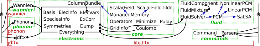
Fig. 1 shows the organization of the key classes and files of the JDFTx codebase, containing 275 source files with approximately 60000 lines of code; this fairly compact implementation for a DFT code is possible because of the algebraic framework discussed above. Most of the functionality is compiled into a dynamic link library libjdftx, which is accessed through light-weight executables jdftx for most calculations, phonon for phonon dispersion and electron-phonon interaction calculations, and wannier for generation of maximally-localized Wannier functions [19] and ab initio tight binding models. This organization makes the procedure straightforward for other DFT codes to leverage JDFTx features, especially JDFT and related solvation models, by linking directly to libjdftx.

The core code (Fig. 1) implements the basic data structures, operators and algorithms used by the rest of JDFTx. ManagedMemory handles data transfers between CPUs and GPUs (automatically, when necessary), and is the base class for ScalarFields and electronic wavefunctions in ColumnBundle. Minimize and Pulay provide algorithms for variational minimization, including linear and nonlinear CG [18], L-BFGS [20]) and self-consistency by Pulay mixing [21]. GridInfo describes the plane-wave grid and Fourier transforms, while Coulomb implements the Coulomb kernel in various dimensions [22].

The fluid code is tied together by the abstract base class FluidSolver, which is implemented by FluidMixure containing several FluidComponents to provide the classical DFTs [12, 23] used for JDFT; see Ref. [12] for more details on this framework to implement atomically-detailed classical DFT for molecular fluids in terms of IdealGas representations and Fex (excess) functionals. Alternately, a hierarchy of solvation models with linear (LinearPCM [24]), nonlinear (NonlinearPCM [16]) and even nonlocal response (SaLSA [25]) derive from base class PCM.

Electronic • Exchange-correlation: semilocal, meta-GGA,
EXX-hybrids, DFT+$U$, DFT-D2, LibXC • Pseudopotentials: norm-conserving and ultrasoft • Noncollinear magnetism / spin-orbit coupling • Algorithms: varitional minimization, SCF • Grand canonical (fixed potential) for electrochemistry • Truncated Coulomb for 0D, 1D, 2D or 3D periodicity • Custom external potentials, electric fields • Charged-defect corrections: bulk and interfacial • Ion/lattice optimization with constraints • Ab initio molecular dynamics • Vibrational modes, phonons and free energies Fluid • Linear solvation: GLSSA13, SCCS, CANDLE • Nonlinear solvation: GLSSA13 • Nonlocal solvation: SALSA • JDFT with classical DFT fluids Outputs (selected) • DOS, optical matrix elements, polarizability etc. • Wannier functions and ab initio tight-binding • Electron-electron and electron-phonon scattering Interfaces • Solvated QMC with CASINO • Atomistic Simulation Environment (NEB, MD etc.) • Visualization: VESTA, XCrySDen, PyMOL

Table 1: Selected features of JDFTx. See index of input file commands on http://jdftx.org for a complete list.

The electronic code contains the standard Kohn-Sham electronic DFT implementation (with class names derived from the original implementation of DFT++ [11]). Here, ElecInfo and ElecVars contain electronic occupations, wavefunctions, density, potential etc. and the functions relating them. SpeciesInfo handles electron-ion interactions (pseudopotentials), ExCorr implements exchange-correlation functionals, and Dump handles outputs and post-processing. All this functionality (including fluids) is tied together into the container class Everything for convenience.

Finally, the commands code (Fig. 1) provides an object-oriented interface to define commands and parse input files. All executables use this module to provide a consistent input file syntax that supports environment variable substitution and modular input files; phonon and wannier support all jdftx commands in addition to those specific to phonon dispersion and Wannier function calculations respectively. Complete description of the classes, files and connections between them is available in the API documentation generated automatically by Doxygen [26] on the JDFTx website, http://jdftx.org.

2.2 Software Functionalities

Table 1 lists a selection of features available in JDFTx. It supports the full range of functionality found in all major electronic DFT software. It has built-in support for several semilocal [27, 28, 29], meta-GGA [30] and EXX-hybrid [31, 32, 33] exchange-correlation functions, with additional functionals available through LibXC [34]. DFT+$U$ [35] and DFT-D2 [36] pair potential dispersion corrections allow for handling localized electrons and van der Waals interactions respectively. JDFTx supports norm-conserving and ultrasoft pseudopotentials in the FHI, UPF and USPP formats, which allows easy interoperability with QE [3] and ABINIT [4]. It automatically installs two well-tested, open-source pseudopotential libraries, GBRV (ultrasoft) [37] and SG15 (norm-conserving) [38], enabling out-of-the-box calculations for most elements. JDFTx supports interactions with custom external potentials and fields, and allows accurate calculations of systems of any dimensionality: molecules (0D), wires (1D), slabs / 2D materials and bulk (3D), using truncated Coulomb interactions [22].

Importantly, JDFTx implements two distinct classes of algorithms for electronic DFT, variational minimization of the (analytically-continued) total energy [39, 40] and the self-consistent field (SCF) iteration method [41]. Variational minimization is stable and guaranteed to converge, while SCF (the default method available in all DFT codes) is less stable in general, but faster when it converges well. JDFTx also uniquely implements grand-canonical DFT [42], where electron number adjusts automatically at a fixed electron chemical potential, which correctly describes the behavior of electrochemical systems. SCF convergence can be problematic in this mode, and for many solvated systems in general; variational minimization is therefore essential to have as an alternative.

JDFTx specializes in electronic structure calculations incorporating a continuum description of the environment, with a the range of techniques available for including fluids and solvation effects. Full JDFT calculations include a detailed classical DFT description of the liquid that captures atomic-scale structure in a number of solvents [43, 12, 23]. JDFTx also includes a hierarchy of solvation models for computationally inexpensive treatment of solvation effects, ranging from the nonlocal solvation model SaLSA [25] which captures atomic-scale liquid structure at a linear-response level, through models that capture nonlinear dielectric and ionic response [16], to the simplest linear-response models [24]. These linear response models include GLSSA13 [16] (later ported to VASP as VASPsol [17]), SCCS [15] (the solvation model available in QE) and CANDLE [44]. Table 2 compares the accuracy of these solvation models for a standard set of neutral solutes, cations and anions in water, and shows that CANDLE achieves the best accuracy for aqueous solvation of charged species by explicitly capturing charge asymmetry in solvation.

Model	MAE [kcal/mol]
	Neutral	Cations	Anions	All
Nonlocal SaLSA [25]	1.36	3.20	19.7	4.55
Nonlinear GLSSA13 [16]	1.28	16.1	27.0	7.55
Linear GLSSA13 [16]	1.27	2.10	15.1	3.59
= VASPsol [17]
SCCS neutral fit 1 [15]	1.20	2.55	17.4	3.97
SCCS neutral fit 2 [15]	1.28	2.66	16.9	3.97
SCCS cation fit [45]	–	2.26	–	–
SCCS anion fit [45]	–	–	5.54	–
CANDLE [44]	1.27	2.62	3.46	1.81

Table 2: Comparison of mean absolute errors (MAE) of solvation energies predicted by various solvation models for an identical set of 240 neutral solutes, 51 cations and 55 anions in water. See Ref. 45 for a detailed specification of individual solutes. CANDLE provides the best accuracy for neutrals, cations and anions within a single parametrization because it explicitly accounts for charge asymmetry in solvation [44].

JDFTx can export a wide-range of electronic structure and liquid properties including charge/site densities, potentials, density of states, vibrational/phonon modes and free energies, optical and electron-phonon matrix elements etc. (See http://jdftx.org/CommandDump.html for a full list.) Executable wannier can generate maximally-localized Wannier functions for either separated or entangled bands [19, 46] and transform Hamiltonians and matrix elements into an ab initio tight-binding model. JDFTx is also interfaced with several commonly-used visualization software packages, and with the Atomistic Simulation Environment [47] for features including Nudged Elastic Band (NEB) [48] barrier calculations and alternate molecular dynamics methods. It provides solvation functionality to other electronic structure software through interfaces, such as for Quantum Monte-Carlo (QMC) simulations in CASINO [49].

3 Illustrative Example

JDFTx is used exactly like most plane-wave DFT software, with an input file that describes the atomic geometry, pseudopotentials, functionals, and other similar options alongside the operations to be performed. For example, Listing 2 shows an input file for a formate ion on a Pt(111) surface, modeled as a 3 layer slab in a 2$\times$2 supercell, with the slab normal along the third lattice vector. The first section selects the GBRV pseudopotentials [37] for all elements (using the wildcard ‘$ID’) and corresponding kinetic energy cutoffs (all energies in Hartrees ($E_{h}$)) for wavefunctions and charge densities. The second section specifies the lattice geometry, slab-mode Coulomb truncation to isolate periodic images along $z$, ionic positions in lattice coordinates, and requests 10 iterations of ionic geometry optimization. The final 0 on the Pt atom positions constrains their positions completely, the 1 allows the rest to move, while ‘Planar 0 0 1’ constrains the C atom to only move in the plane normal to the third lattice vector.

Listing 2: JDFTx input file demonstrating several useful features: fixed-potential calculation of a formate ion on Pt(111) using the CANDLE solvation model for a 1M aqueous NaF electrolyte, geometry optimization with Pt positions and $z$ coordinate of C constrained, and with electron density and fluid bound charge output.

⬇

#--- Pseudopotentials ---

ion-species GBRV/$ID_pbe_v1.2.uspp #GBRV family

ion-species GBRV/$ID_pbe_v1.uspp #GBRV family

elec-cutoff 20 100 #Ecuts for psi and rho

#--- Geometry ---

lattice Hexagonal 10.53 30.0 #a and c in bohrs

coulomb-interaction Slab 001 #Make z nonperiodic

coulomb-truncation-embed 0 0 0 #Specify center

coords-type Lattice #fractional coordinates

ion Pt 0.33333 -0.33333 -0.288 0

ion Pt 0.33333 -0.83333 -0.288 0

ion Pt 0.83333 -0.83333 -0.288 0

ion Pt 0.83333 -0.33333 -0.288 0

ion Pt 0.16667 -0.16667 -0.144 0

ion Pt 0.16667 -0.66667 -0.144 0

ion Pt 0.66667 -0.16667 -0.144 0

ion Pt 0.66667 -0.66667 -0.144 0

ion Pt 0.000 0.000 0.000 0

ion Pt 0.000 -0.500 0.000 0

ion Pt 0.500 0.000 0.000 0

ion Pt 0.500 -0.500 0.000 0 #0 => fixed

ion O 0.152 -0.079 0.155 1 #1 => free

ion O -0.152 +0.079 0.155 1

ion C 0.000 0.000 0.190 1 Planar 0 0 1

ion H 0.000 0.000 0.260 1

ionic-minimize nIterations 10 #Optimize geometry

#--- Electronic ---

kpoint-folding 6 6 1 #Gamma-centered k-mesh

elec-smearing Cold 0.01 #Select cold smearing

target-mu -0.160 #Fix echem potential

#--- Fluid ---

fluid LinearPCM #Class of solvation model

pcm-variant CANDLE #Specific model within class

fluid-solvent H2O #Aqueous electrolyte

fluid-cation Na+ 1. #1 mol/L Na+ cation

fluid-anion F- 1. #1 mol/L F- anion

#--- Outputs ---

dump Ionic IonicPositions ElecDensity BoundCharge

dump-name test.$VAR #Output filename pattern

The third section of Listing 2 selects Brillouin zone sampling, smearing, and a unique feature of JDFTx: grand canonical DFT [42] at a fixed electron chemical potential $\mu=-0.16~{}E_{h}$. The fourth section selects the CANDLE solvation model [44] for water with 1M (mol/L) Na+ and F- ions. The final section requests output every ionic step of ionic positions, electron density and bound charge density in the fluid, with files named using the pattern ‘test.*’. The organization above is only for illustration; commands may appear in any order, may be split over multiple input files with ‘include’ statements, and may invoke environment variable substitution for ease of scripting. See http://jdftx.org/Commands.html for more details.

Figure 2: Visualization of the structure along with (a) electron density and (b) fluid bound charge density from the results of running JDFTx on the input in Listing 2, generated using the createXSF script (distributed with JDFTx) and VESTA [50].

After saving Listing 2 to ‘test.in’ (as one possible naming convention),

⬇

mpirun -n 4 jdftx -c8 -i test.in -o test.out

runs the code using 4 MPI processes with 8 threads each, logging output to ‘test.out’. After completion,

⬇

createXSF test.out test.xsf n

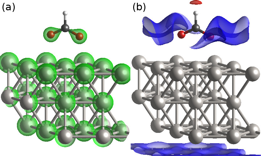
creates file ‘test.xsf’ containing the structure and electron density $n(\vec{r})$, which visualized in VESTA [50] yields Figure 2(a). The same procedure with ‘nbound’ instead of ‘n’ yields Figure 2(b) that shows the bound charge density in the fluid. As expected, the formate electron density (green) is greatest on the O atoms, surrounded by a positive (blue) fluid bound charge. A small negative (red) bound charge appears next to the H, but at this potential the Pt surface is negatively charged and mostly surrounded by positive charge in the fluid. (The raw output from JDFTx uses the opposite electron-is-positive sign convention rather than the usual convention employed in this discussion.)

Figure 3: Variation of JDFTx run time with number of MPI processes for (a) the initial vacuum DFT and (b) for the subsequent grand canonical solvated DFT at the initial geometry for the calculation specified by Listing 2. Each CPU process runs on one 8-core Intel Xeon E5-2620v4 socket (two sockets per compute node), while each GPU process runs on one NVIDIA Tesla K80 GPU (two GPUs per K80 unit). Dotted lines indicate ideal linear scaling. (The marginal super-linear speedup for CPU processes in (a) is due to increased ratio of cache size to memory used per process.)

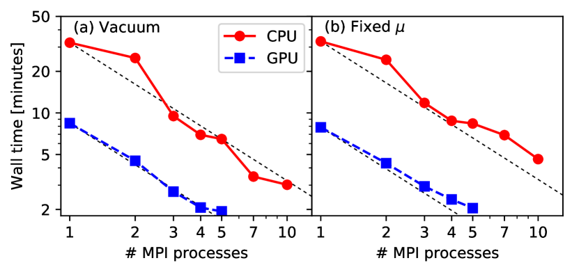
Figure 3 illustrates the performance of JDFTx using the above example for both (a) conventional vacuum DFT calculations (performed automatically before solvated calculations) and (b) fixed-potential solvated calculations, on varying numbers of both CPUs and GPUs. JDFTx implements MPI parallelization over symmetry-reduced $k$-points and pthreads / CUDA parallelization over everything else. It exhibits almost linear MPI scaling when the number of processes is a factor of this $k$-point count (20 in above example). Each K80 GPU delivers approximately $3\times$ performance compared to each 8-core Xeon approximately ($25\times$ compared to each core) for this problem size.

4 Impact

JDFTx simultaneously targets two partially-overlapping research communities: developers of new DFT methods, models, and algorithms, and DFT practitioners who take advantage of these new methods. It emphasizes ease of development as well as use, realized in practice with highly-modular code that expresses physics in almost the same language as the theoretical derivations, using the algebraic formulation of DFT and an efficient C++11 abstraction, as discussed above. Using this framework, we have rapidly implemented in a few years a complete feature set comparable to that of proprietary codes that have been in development for decades, making JDFTx now usable as a general-purpose DFT software.

JDFTx has facilitated the rapid development of new methods for a number of applications, most notably for DFT calculations of solvated and electrochemical systems using JDFT [10] and solvation models. JDFTx served as the medium for development of liquid free energy functionals (classical DFT functionals) [43, 12, 23] to realize JDFT, as well as a hierarchy of increasingly accurate solvation models including simple linear solvation models [24, 16, 51], nonlinear models [16, 52, 53] and models incorporating nonlocality: SaLSA [25] and CANDLE [44]. In fact, one of the simplest models developed using JDFTx, GLSSA13 [16], was later ported to the proprietary DFT code VASP as VASPsol [17], the predominant solvation option for that code. Solvation from JDFTx can be used for quantum Monte Carlo simulations through an interface with the CASINO code [49, 54]. JDFTx recently enabled the development of grand-canonical DFT algorithms [42], making it possible to realistically simulate electrochemical processes by allowing number of electrons in the calculation to adjust automatically at fixed potential. More generally, JDFTx has also been used in electronic structure method development for exact exchange [22], dielectric matrices [55], X-ray measurements [56],and electron-phonon interactions [57].

JDFTx makes these cutting-edge methods immediately available in efficient, easy-to-use code for a wide spectrum of applications. JDFT and solvation techniques in JDFTx have already been used to elucidate ion distribution [58] and dendrite formation [59, 60] in Li ion batteries, surface structures and reaction mechanisms for various energy-conversion catalysts [56, 61, 62, 63, 64, 65, 66], new electrode materials for supercapacitors [67, 68, 69], prediction of electrochemical pseudocapacitance [70], and band alignments at solid-liquid interfaces [71, 72], to take just a few prominent examples. JDFTx has also facilitated Wannier-function based ab initio tight-binding calculations of photo-excited hot carrier generation [73, 57, 74, 75], transport [76, 77, 78] and ultrafast dynamics [79, 80]. Continuing development of new interfaces and multi-scale methods using JDFTx will expand the range of applications further.

5 Conclusions

We present JDFTx, a general-purpose open-source plane-wave DFT software, with a particularly rich feature set for solvated and electrochemical DFT calculations, and with an emphasis on ease of development and use. In its first five years, JDFTx has enabled rapid development of joint density-functional theory (JDFT) and a hierarchy of efficient and accurate solvation models, which are gradually being implemented or interfaced with proprietary and other open-source DFT codes. With these methods, JDFTx has already been widely applied to electrochemical problems in catalysis, energy conversion and energy storage.

The design of JDFTx allows short, easy-to-read code to perform well on various hardware architectures, making it ideally suited to rapidly prototype new methods, and then test and optimize them. All functionality is exposed as a library, libjdftx, that other software can link to for direct interfacing. Future interfaces of JDFTx with other open-source software for electronic structure calculations, direct computation of experimental observables, electromagnetic simulations, phase-field methods, and more will drive widespread applications of multi-scale techniques that start at the electronic scale.

Required Metadata

C1	Current code version	1.3.1
C2	Permanent link to code/repository used for this code version	https://github.com/shankar1729/jdftx/releases/tag/v1.3.1
C3	Legal Code License	GPLv3
C4	Code versioning system used	git
C5	Software code languages, tools, and services used	C++11, MPI, CUDA
C6	Compilation requirements, operating environments & dependencies	GSL, BLAS, LAPACK and FFTW libraries on a POSIX-compliant platform
C7	Link to developer documentation/manual	http://jdftx.org
C8	Support email for questions	sundar@rpi.edu

Table 3: Code metadata

S1	Current software version	1.3.1
S2	Permanent link to executables of this version	https://github.com/shankar1729/jdftx/archive/v1.3.1.zip
S3	Legal Software License	GPLv3
S4	Computing platforms/Operating Systems	POSIX-compliant platform (Linux, Unix, OS X, Windows/Cygwin etc.)
S5	Installation requirements & dependencies	MPI C++11 compiler; GSL, BLAS, LAPACK and FFTW libraries
S6	Link to user manual	http://jdftx.org
S7	Support email for questions	sundar@rpi.edu

Table 4: Software metadata

References

- [1] M. J. Frisch, G. W. Trucks, H. B. Schlegel, et al., Gaussian 09, Gaussian Inc. Wallingford CT 2009.
- [2] G. Kresse, J. Furthmüller, Comput. Mater. Sci. 6 (1996) 15–50.
- [3] P. Giannozzi, S. Baroni, N. Bonini, M. Calandra, R. Car, C. Cavazzoni, et al., J. Phys.: Condens. Matter 21 (2009) 395502.
- [4] X. Gonze, J.-M. Beuken, R. Caracas, F. Detraux, M. Fuchs, G.-M. Rignanese, et al., Comp. Mater. Sci. 25 (2002) 478.
- [5] F. Gygi, IBM J. Res. Dev. 52 (2008) 137.
- [6] X. Xu, W. A. Goddard, J. Chem. Phys. 121 (2004) 4068.
- [7] K. Jarolimek, E. Hazrati, R. A. de Groot, G. A. de Wijs, Phys. Rev. Applied 8 (2017) 014026.
- [8] R. Car, M. Parrinello, Phys. Rev. Lett. 55 (1985) 2471.
- [9] J. J. Wu, Classical Density Functional Theory for Molecular Systems, Springer, Singapore, 2017, p. 65.
- [10] S. A. Petrosyan, J.-F. Briere, D. Roundy, T. A. Arias, Phys. Rev. B 75 (2007) 205105.
- [11] S. Ismail-Beigi, T. A. Arias, Comp. Phys. Comm. 128 (2000) 1.
- [12] R. Sundararaman, T. Arias, Comp. Phys. Comm. 185 (2014) 818.
- [13] W. Kohn, L. Sham, Phys. Rev. 140 (1965) A1133.
- [14] A. V. Marenich, C. J. Cramer, D. G. Truhlar, J. Phys. Chem. B 113 (2009) 6378.
- [15] O. Andreussi, I. Dabo, N. Marzari, J. Chem. Phys 136 (2012) 064102.
- [16] D. Gunceler, K. Letchworth-Weaver, R. Sundararaman, K. Schwarz, T. A. Arias, Modelling Simul. Mater. Sci. Eng. 21 (2013) 074005.
- [17] K. Matthew, R. Sundararaman, K. Letchworth-Weaver, T. A. Arias, R. G. Hennig, J. Chem. Phys. 140 (2014) 084106.
- [18] R. Fletcher, C. M. Reeves, Comp. J. 7 (1964) 149.
- [19] N. Marzari, D. Vanderbilt, Phys. Rev. B 56 (1997) 12847.
- [20] D. C. Liu, J. Nocedal, Math. Program. 45 (1989) 503.
- [21] P. Pulay, Mol. Phys. 17 (1969) 197.
- [22] R. Sundararaman, T. A. Arias, Phys. Rev. B 87 (2013) 165122.
- [23] R. Sundararaman, K. Letchworth-Weaver, T. A. Arias, J . Chem. Phys. 140 (2014) 144504.
- [24] K. Letchworth-Weaver, T. A. Arias, Phys. Rev. B 86 (2012) 075140.
- [25] R. Sundararaman, K. A. Schwarz, K. Letchworth-Weaver, T. A. Arias, J. Chem. Phys. 142 (2015) 054102.
- [26] D. van Heesch, Doxygen, http://www.doxygen.org.
- [27] J. P. Perdew, A. Zunger, Phys. Rev. B 23 (1981) 5048.
- [28] J. P. Perdew, K. Burke, M. Ernzerhof, Phys. Rev. Lett. 77 (1996) 3865.
- [29] J. P. Perdew, et al., Phys. Rev. Lett. 100 (2008) 136406.
- [30] J. P. Perdew, A. Ruzsinszky, G. I. Csonka, L. A. Constantin, J. Sun, Phys. Rev. Lett. 103 (2009) 026403.
- [31] C. Adamo, V. Barone, J. Phys. Chem. 110 (1999) 6158.
- [32] A. V. Krukau, O. A. Vydrov, A. F. Izmaylov, G. E. Scuseria, J. Chem. Phys 125 (2006) 224106.
- [33] J. E. Moussa, P. A. Schultz, J. R. Chelikowsky, J. Chem. Phys. 136 (2012) 204117.
- [34] M. A. L. Marques, M. J. T. Oliveira, T. Burnus, Comput. Phys. Commun. 183 (2012) 2272.
- [35] S. L. Dudarev, G. A. Botton, S. Y. Savrasov, C. J. Humphreys, A. P. Sutton, Phys. Rev. B 57 (1998) 1505.
- [36] S. Grimme, J. Comput. Chem 27 (2006) 1787.
- [37] K. F. Garrity, J. W. Bennett, K. Rabe, D. Vanderbilt, Comput. Mater. Sci. 81 (2014) 446.
- [38] M. Schlipf, F. Gygi, Comput. Phys. Commun. 196 (2015) 36.
- [39] T. A. Arias, M. C. Payne, J. D. Joannopoulos, Phys. Rev. Lett. 69 (1992) 1077.
- [40] C. Freysoldt, S. Boeck, J. Neugebauer, Phys. Rev. B 79 (2009) 241103(R).
- [41] G. Kresse, J. Furthmüller, Phys. Rev. B 54 (1996) 11169.
- [42] R. Sundararaman, W. A. Goddard III, T. A. Arias, J. Chem. Phys. 146 (2017) 114104.
- [43] R. Sundararaman, K. Letchworth-Weaver, T. A. Arias, J . Chem. Phys. 137 (2012) 044107.
- [44] R. Sundararaman, W. A. Goddard III, J. Chem. Phys. 142 (2015) 064107.
- [45] C. Dupont, O. Andreussi, N. Marzari, J. Chem. Phys 139 (2013) 214110.
- [46] I. Souza, N. Marzari, D. Vanderbilt, Phys. Rev. B 65 (2001) 035109.
- [47] A. H. Larsen, J. J. Mortensen, J. Blomqvist, I. E. Castelli, R. Christensen, M. Dulak, et al., J. Phys.: Cond. Matt. 29 (2017) 273002.
- [48] G. Henkelman, B. Uberuaga, H. Jonsson 113 (2000) 9901.
- [49] R. J. Needs, M. D. Towler, N. D. Drummond, P. L. Ríos, J. Phys.: Condens. Matter 22 (2010) 023201.
- [50] K. Momma, F. Izumi, J. Appl. Crystallogr. 44 (2011) 1272.
- [51] R. Sundararaman, K. A. Schwarz, J. Chem. Phys. 146 (2017) 084111.
- [52] R. Sundararaman, D. Gunceler, T. A. Arias, J. Chem. Phys. 141 (2014) 134105.
- [53] D. Gunceler, T. A. Arias, Modelling Simul. Mater. Sci. Eng. 25 (2017) 015004.
- [54] K. A. Schwarz, R. Sundararaman, K. Letchworth-Weaver, T. A. Arias, R. G. Hennig, Phys. Rev. B 85 (2012) 201102(R).
- [55] K. Schwarz, R. Sundararaman, T. A. Arias, J. Chem. Phys. 142.
- [56] M. Plaza, X. Huang, J. Y. P. Ko, M. Shen, B. H. Simpson, J. Rodríguez-López, et al., J. Am. Chem. Soc. 138 (2016) 7816.
- [57] A. Brown, R. Sundararaman, P. Narang, W. A. Goddard III, H. A. Atwater, ACS Nano 10 (2016) 957.
- [58] M. E. Holtz, Y. Yu, D. Gunceler, J. Gao, R. Sundararaman, K. A. Schwarz, T. A. Arias, H. D. Abruna, D. A. Muller, Nano Lett. 14 (2014) 1453.
- [59] Y. Ozhabes, D. Gunceler, T. A. Arias, Stability and surface diffusion at lithium-electrolyte interphases with connections to dendrite suppression, arXiv:1504.05799.
- [60] S. Choudhury, Z. Tub, S. Stalina, D. Vua, K. Fawolea, D.Gunceler, et al., Angew. Chem. Int. Ed. 56 (2017) 13070.
- [61] K. A. Schwarz, R. Sundararaman, T. P. Moffat, T. Allison, Phys. Chem. Chem. Phys. 17 (2015) 20805.
- [62] K. A. Schwarz, B. Xu, Y. Yan, R. Sundararaman, Phys. Chem. Chem. Phys. 18 (2016) 16216.
- [63] H. Xiao, T. Cheng, W. A. Goddard III, R. Sundararaman, J. Am. Chem. Soc. 138 (2016) 483.
- [64] Y. Ping, R. J. Nielsen, W. A. Goddard III, J. Am. Chem. Soc. 139 (2017) 149.
- [65] H. Zhuang, A. J. Tkalych, E. A. Carter, J. Phys. Chem. C 120 (2016) 23698.
- [66] N. Z. Koocher, D. Saldana-Greco, F. Wang, S. Liu, A. M. Rappe, The Journal of Physical Chemistry Letters 6 (2015) 4371.
- [67] S. Sun, Y. Qi, T.-Y. Zhang, Electrochimica Acta 163 (2015) 296.
- [68] C. Zhan, D. Jiang, J. Phys. Chem. Lett. 7 (2016) 789.
- [69] C. Zhan, P. Zhang, S. Dai, D. Jiang, ACS Energy Lett. 1 (2016) 1241.
- [70] C. Zhan, D. Jiang, J. Phys.: Condens. Matter 28 (2016) 464004.
- [71] Y. Ping, R. Sundararaman, W. A. Goddard III, Phys. Chem. Chem. Phys. 17 (2015) 30499.
- [72] R. Sundararaman, Y. Ping, J. Chem. Phys. 146 (10).
- [73] R. Sundararaman, P. Narang, A. Jermyn, W. A. Goddard III, H. A. Atwater, Nat. Comm. 5 (2014) 5788.
- [74] P. Narang, R. Sundararaman, A. Jermyn, W. A. Goddard III, H. A. Atwater, J. Phys. Chem. C 120 (2016) 21056.
- [75] P. Narang, R. Sundararaman, H. A. Atwater, Nanophotonics 5 (2016) 96.
- [76] P. Narang, L. Zhao, S. Claybrook, R. Sundararaman, Adv. Opt. Mater. 5 (2017) 1600914.
- [77] E. Cortes, W. Xie, J. Cambiasso, A. Jermyn, R. Sundararaman, P. Narang, et al., Nature Commun. 8 (2017) 14880.
- [78] A. Jermyn, G. Tagliabue, H. A. Atwater, W. A. Goddard III, P. Narang, R. Sundararaman, Far-from-equilibrium transport of excited carriers in nanostructures, arXiv:1707.07060 (2017).
- [79] A. Brown, R. Sundararaman, P. Narang, W. A. Goddard III, H. A. Atwater, Phys. Rev. B 94 (2016) 075120.
- [80] A. Brown, R. Sundararaman, P. Narang, A. Schwartzberg, W. A. Goddard III, H. A. Atwater, Phys. Rev. Lett. 118 (2017) 087401.