Muon pair production with hadronic vacuum polarization re-evaluated using precise data fits

Abstract

Using optical theorem within sophisticated fits for exclusive hadronic productions in $e^{+}e^{-}$ collisions the interference between leptonic and hadronic vacuum polarization functions is considered and applied for calculation of $\mu-$pair productions below 3 GeV. Particularly, the dispersion relation for the pion production form factor was obtained, confirming a possible evidence for the light $\rho(1250)$ resonance. The inflated error was introduced and used to discriminate the quality of various phenomenological fits. Resulting hadronic vacuum polarization was compared with other conventional sources and compared with KLOE experiment for $\mu^{-}\mu^{+}$ production at $\phi$ meson energy. Furthermore, the obtained running fine structure coupling is compared with KLOE2 experiment for radiative return $\mu^{-}\mu^{+}$ production at $\omega/\rho$ meson energy and careful analysis of the error stemming form various fits of combined data was made and discussed.

I Introduction

Comparisons between theory and experiment are used to test Standard Theory for decades. For an accurate measurement the studies require consistent account of leptonic as well as hadronic virtual corrections. The hadronic contribution to photon vacuum polarization function plays particularly important role, since it is the main source of uncertainties in theoretical calculation of muon anomalous magnetic moment $a_{\mu}$. The last precise measurement of $a_{\mu}$, together with the last decades data for electrohadron production, confirms the evidence of tension between Standard Theory and experiments amu1 ; amu2 ; Abi2021 . Similar confrontation of the theoretical technique with the experimental accuracy is offered by observed AUGU1973 ; BERKOM1976 interference effect between leptonic and hadronic vacuum polarization functions at energies of narrow resonances: $\omega$ and $\phi$ and heavier quarkonia $J/\psi,\Psi$ and $\Upsilon$’s. There, the total cross section $\sigma_{h}$ is enhanced several orders of magnitude when compared to other region of energy. In practice, the effect is explored in the so called B-factories like BABAR, BELLE or BESS or more earlier in Frascati where detectors and accelerator are tuned for $\Upsilon$ or $\phi$ meson energy. Narrow mesons off prints in the vacuum polarization turns to be a measurable fluctuation in the QED running coupling- the electromagnetic decay of mesons. This effect is presented in the all electromagnetic processes, being most easily observed in a single Mandelstam variable $s$-dependent process, e.g. the muon pair production. The most recent precise measurements of muon production $e^{+}e^{-}\to\mu^{+}\mu^{-}$ by SND, CMD-2,3 and the KLOE(2) detectors represent another possible stringent test of the Standard Theory. In this case, the theory and experiment comparison means to compare the whole shape of energy dependent functions.

With incomes of many new precise data for the cross section $\sigma_{h}$ we reanalyzed the calculation for AMBRO2005 within the use polarization function obtained by groups polar2 ; polar3 as well as by independent calculation performed here. Further, having extracted hadron polarization function, we provide independent comparison of theory and recent KLOE2 KLOEdva measurement of the fine structure coupling constant.

Particularly, we performed the fit for amplitudes of all necessary hadronic cross sections with emphasizing on two pions channel, for which we compare two rather different approaches. The $\pi\pi$ production cross section represents the most dominant hadronic contribution ( 75 $\%$) to the muon anomalous moment and it should contain important information about spectra of $1^{-}$ vector meson resonances. Notably, albeit only for spacelike momentum $Q^{2}$, it involves the form factor function, which has been calculated from Schwinger-Dyson equations (the nonperturbative set of equation for Green’s functions). At opposite -timelike- momentum axis, the position and the ordering of resonances is believed to be important for understanding of confinement issue. Let us remain the old-fashionable quantum mechanical picture of linear Regge trajectories $M^{2}(N)$ where $N$ is radial number of the resonance. In this respect a recent evidence for very wide resonance $\rho(1250)$ from the unitary multichannel reanalysis rupp of elastic pion scattering is in a certain contradiction with the modern Schwinger-Dyson equations studies (see for instance HGK2017 ). For this purpose we write down the dispersion relation for the pion form factor and fit the spectral function. Reduction of number of parameters needed for such a description shows the right analytical form has been chosen in this case. As a matter of the fact, making a precise fit of combined data form several most important experiments, our results indicate a broad vector meson like structure in the range $1.15-1.3GeV$. It is also shown that non-resonant background plays an important role in the description.

II $\sigma_{\mu\mu}$ for KLOE 2004

The theory and the comparison between calculated cross section $\sigma_{\mu\mu}=\sigma(e^{+}e^{-}\to\mu^{+}\mu^{-})$ and the high precision measurement obtained by KLOE detector AMBRO2005 is presented in this section.

The integrated cross section, for which we adopt approximation and conventions given by ARBU1997 , can be written in the following way

$$\sigma(s)=\frac{4\pi C_{t}}{\left|1-\Pi(s)\right|^{2}}\left[\sigma_{A}(s)\left(2-\beta_{\mu}^{2}(1-\frac{C_{t}^{2}}{3})\right)+\sigma_{B}(s)\right]\,,$$ (1)

where $C_{t}$ stand for $\cos(\theta_{min})$ with $\theta_{min}=50^{0}$ ($\theta_{max}=140^{o}$), which is KLOE experimental cut on polar scattering angle between $\mu^{-}$ and $e^{-}$ particles and $\beta_{\mu}=\sqrt{1-4m^{2}_{\mu}/s}$. The function $\sigma_{A}(s)$ is defined such that it has an angular dependence identical to the Born cross section. The rest is unique and explicitly reads

$$\sigma_{B}(s)=-\frac{\alpha^{3}}{4\pi s}(1-\beta_{\mu}^{2})\ln{\frac{1+\beta_{\mu}}{1-\beta_{\mu}}}\,.$$ (2)

Thus the main term $\sigma_{A}(s)$, listed completely in ARBU1997 , collects all leading logs of Dirac and Pauli form factors and the known soft photon contributions for which we take $ln\frac{\Delta\epsilon}{\epsilon}=0.05$ (15 MeV cut on c.m.s. soft photon energy at $\phi$ peak). Let us mention that the the both $\sigma_{A}$ as well as $\sigma_{B}$ are slowly changing real valued functions and do not play an important role in the observed interference effect.

The integral cross section formula is proportional to the square of the fine structure constant $\alpha(s)$, which reads

$$\alpha(s)=\frac{\alpha}{1-\Pi(s)}\,,$$ (3)

with $\alpha=\alpha(0)=1/137.0359991390$ and where the polarization function $\Pi(s)=\Pi_{l}(s)+\Pi_{h}(s)$ is completed from the leptonic $l$ and the hadronic $h$ part.

Purely QED contributions are well known from perturbation theory. Since, there are some mistakes in the formula in Ref. ARBU1997 , I present leptonic contribution into the vacuum polarization function here:

$$\Pi_{l}(s)=\frac{\alpha}{\pi}\Pi_{1}(s)+\left(\frac{\alpha}{\pi}\right)^{2}\Pi_{2e}(s)\,\,,$$ (4)

where one loop contribution is

$$\Pi_{1}(s) = \Pi_{e}(s)+\Pi_{\mu}(s)+\Pi_{\tau}(s)\,\,;$$

$$\Pi_{f}(s) = -5/9-x_{f}/3+f(x_{f})\,\,;f=e,\mu,\tau\,;$$

$$f(x_{f}) = \frac{\beta_{f}}{6}(2+x_{f})\left(\ln{\frac{1+\beta_{f}}{1-\beta_{f}}}-i\pi\right)\Theta(1-x_{f})$$ (5)

$$+ \frac{\beta_{f}}{3}(2+x_{f})arctg\left({\frac{1}{\beta_{f}}}\right)\Theta(x_{f}-1)\,\,,$$

where $\beta_{f}=\sqrt{|1-x_{f}|}$ and $x_{f}=4m^{2}_{f}/s$. Also the leading logarithmic term:

$$\Pi_{2e}(s)=\frac{1}{4}ln(\frac{s}{m_{e}^{2}}-i\pi)+\zeta(3)-5/24\,,$$ (6)

which stems from the second order is taken into account (for heavy quarks and large $q^{2}$ one can employ perturbation theory as well, remind only the usual extra factor $\alpha\rightarrow\alpha N_{c}e_{q}^{2}$ in the appropriate one loop expression).

Hadronic part of the polarization function $\Pi_{h}$ is in principle directly calculable from the equations of motions GFW2011 ; sauli2020 where the later approach provides the first, albeit partially incomplete result in the entire Minkowski space. In approaches GFW2011 ; sauli2020 , HVP is calculated from the Standard Model parameters,i.e. without a large use of experimental data. Due to required high accuracy, here we follow the old-fashionable approach and by using the Unitarity, the function $\Pi_{h}$ is extracted from the total hadronic production $\sigma_{h}=\sigma_{tot}(e^{+}e^{-}\rightarrow hadrons)$ and HVP is obtained from the following dispersion relation CABGAT1961 ; EIDJEg1995 :

$$\Pi_{h}(s)=\frac{s}{4\pi^{2}\alpha}\int_{m_{\pi}^{2}}^{\infty}d\omega\frac{\sigma_{h}(\omega)\left[\frac{\alpha}{\alpha(\omega)}\right]^{2}}{\omega-s+i\epsilon}\,.$$ (7)

Since the measurement of low energy inclusive cross section $\sigma_{h}$ is technically demanding, the knowledge of $\sigma_{h}$ relies on many experimental measurements of the hadronic exclusive (hex) processes $\sigma_{hex}$, which constitute $\sigma_{h}$

$$\sigma_{h}=\sum_{hex}\sigma_{hex}\,\,,$$ (8)

noting the photons emitted from the final hadronic states counts as well.

The expression (7) represents a nonlinear integral equation with the singular kernel and to this point, there are only few groups polar2 ; polar3 ; DAVIER2011 , which steadily collect necessary data on $\sigma_{h}$ and provide fresh and more accurate look at the $\Pi_{h}$ line-shape. Before providing the result we describe the determination of $\sigma_{h}$ in our case.

First of all, we follow a common practice and very narrow resonances like heavy quarkonia replace by their Breit-Wigner functions with PDG parameters. The inclusion of the entire rest of $\sigma_{h}$ is included numerically and represent the core of the method. Since the kernel in Eq. (7) is singular a straight use of experimental data would lead to uncontrolled numerical noise and lost of accuracy. In order to make the integration under control we construct the analytic fit of $\sigma_{h}$ as a first step. We established the inflated error in the next section with main concern on the the exclusive cross section $\sigma_{\pi^{+}\pi^{-}}$ for which we construct our own fit based on spectral representation.

III Fit for $\sigma_{h}$ and the inflated error

Mutual incompatibilities in data originating from various experiment usually appear when combining and fitting the data from several different experiments. They originate in different systematical data errors, being always presented due to the different experimental set up and as a consequence the standard fit criterion $\chi^{2}\simeq 1$ turns to be problematic to fullfill for combined data.

Remind the reader, there are basically two methods to determine experimental hadronic cross section $\sigma_{h}$, the first method scan energy intervals and measure the hadronic cross section directly. The second one uses radiative return, being also named Initial State Radiation (ISR) method, wherein the $n$-body hadronic cross section is extracted from $n+1$-body final hadron+photon cross section. The advantage of the later is minimized background and the access to an amazingly large range of $s$ in single experiment.

To be able to calculate the propagation of experimental errors, a successful introduction of semi-stochastic inflated error (IE) is needed. Suitably defined inflated error $\sigma_{I}$ then can partially accounts (even not well determined) systematic error in a statistical manner. Since there does not exist a unique definition in the literature, we are going to define the IE through the fit $\sigma_{fit}$ of data $\sigma_{h}$ : the IE $\sigma_{I}$ is defined such that we get minimal $\chi_{I}^{2}=1$ in a theoretically allowed space of functions $\sigma_{fit}$ and $\sigma_{I}$ and simultaneously $\sigma_{I}$ is smallest for all variables (energy $E_{i}$ in our case). More concretely, $\chi^{2}$ is obtained through minimization of the following quantity

$$\chi_{I}^{2}=\sum_{i}\frac{[\sigma_{h}(E_{i})-\sigma_{fit}(E_{i})]^{2}}{\sigma_{I}^{2}(E_{i})}^{2}\,.$$ (9)

where $E_{i}$ is the energy of positron-electron pair and $i$ runs over all data points.

Obviously, the introduced IE replaces the statistical error $\sigma_{stat}$ of single experiment and therefore as the additional requirement we impose the condition

$$\sigma_{stat}<\sigma_{I}$$ (10)

at all points $E_{i}$. Such a construction automatically ensures that we must get an upper estimate of statistical error when single experiment is considered. In general case, one should expect that $\sigma_{I}\simeq\sigma_{tot}=\sqrt{\sigma_{stat.}^{2}+\sigma_{syst}^{2}}$ for many experiments with comparable accuracy. In this respect the systematical errors are regarded as the additional noise. Of course, in case of small number of experiments, or in case of correlated experiments, the effect of systematical error should not be ignored and should be discussed separately.

In suggested approach here, the IE is established simultaneously with the cross section fit $\sigma_{fit}$ for each set of measured hadronic exclusive data. More concretely we take

$$\sigma_{I}(s)=c_{I}\sqrt{\sigma_{fit}(s)}$$ (11)

with a constant energy independent coefficient $c_{I}\simeq 1nb^{1/2}$. It provides all required properties we need for modern data on $\sigma_{h}$ bellow $3GeV$. We are satisfied with a single definition of the inflated error, however reaching a higher energies a split to several definitions of IEs, each valid only for a certain interval could be done in order to reflect accuracy at regions dominated by quarkonia.

Due to the simple choice (11), the value $c_{I}$ is therefore one of the main, but not unique, criterion of the quality of the data fir bellow $3GeV$. Depending on required or assumed fit properties (analyticity, spectrality, unitarity etc) there can exist more best fits due to other possible constrains. Therefore associated fits can have their own and in-equivalent IEs, nevertheless one can compare them quantitatively by achieved constants $c_{I}$. Alternatively one can evaluate the fit of “theory 1” with the error achieved by another fit and compare their $\chi^{2}$ mutually. Of course, the experimental statistical error can serve for comparison of various fits as well, albeit the associated error is underestimated, since counts only with individual statistical errors of principally different experiments. For purpose of labeling we will use $\chi_{D}$ in order to distinguish from other $\chi^{2}$.

IV $\pi\pi$ contribution to $\sigma_{h}$ via analytical pion form factor $F$ and evidence of $\rho(1250)$

,

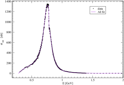
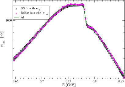
Figure 1: $\sigma_{\pi\pi}$ cross section Left: All combined data and the best spectral fit as described in text. Right: Here we show fits at $\rho$ peak position. GS fit evaluated at all data points with inflated error is shown (light lines for errors). For comparison the BaBaR data with the total error are shown. The best spectral fit is shown as well (single black solid line). Errors are not shown for the later case in order to keep other points visible.

We describe the fit for $\pi\pi$ production cross section in this Section. Likewise in method used in rupp ; BYKANA2016 ; BOLD2017 we impose a constrain and write down the fit for the amplitude. For this purpose the spectral representation is chosen for the pion form factor, which also involves meson $\rho(1250)$ with three other more conventional excited states of vector mesons. Imposing further constrains, which radically reduce the number of free parameters, still the excellent agreement with the data was found. It provides the inflated error determined by the constant $c_{I}^{2}=0.36nb$, being thus substantial smaller then the result achieved previously in earlier analyses SAHVP1 ; SAHVP2 , where we got $c_{I}^{2}=0.64nb$.

The pion electromagnetic form factor $F_{\pi}$ is conventionally defined through measured hadronic cross section

$$\sigma_{\pi\pi}(q)=\frac{\alpha^{2}\pi\beta^{3}}{3s}F_{\pi}^{2}(q)\,,$$ (12)

i.e. with the vacuum polarization included in the form factor $F$.

Here we assume that the entire pion form factor has a real branch point corresponding to the two pionic threshold and therefore can be written in the form of the dispersion relation

$$F_{\pi}(q)=\frac{1}{\pi}\int_{4m_{\pi}^{2}}^{\infty}\frac{\rho_{F}(a)}{q^{2}-a+i\epsilon}\,.$$ (13)

Thus this is the absorptive part $\Im F=-\rho_{F}$ which only needs to be known to determine $F$ entirely. There is no any deep theoretical reason for the analytic behavior dictated be single variable dispersion (13) in QCD, however a similar dispersion relation are known to be working in QCD/QED processes and provide a good agreement with experiments even for more complicated kinematics HOST2019 .

We do not calculate $F$ as we are unawared about working theoretical model which can provide correct result for energy above 1 GeV, but we make a simple fit, which allows us to identify vector resonances involved in the process. The heart of the fitting function for the pion charged form factor is the vector dominance model with sort of dressed Breit -Wigner peaks representing the resonances, which within non-resonant background function $D_{bg}$ completes the result.

We look for spectral function $\rho_{F}$ , which is searched in the following form

$$\rho_{F}(a)=\Im\left\{{\cal D}_{bg}(a)\left[{\cal W}^{GS}_{\rho}(a,m_{\rho},\Gamma_{\rho})(s)\frac{1+c_{\omega}{\cal W}_{\omega}(a,m_{\omega})}{1+c_{\omega}}+\sum_{i}c_{\rho^{i}}{\cal W}^{GS}_{\rho^{i}}(a,m_{\rho^{i}},\Gamma_{\rho^{i}})\right]\right\}\,\,.$$ (14)

where $c$ are real coefficients and two parametric function ${\cal W}^{GS}_{\rho^{i}}$ is listed in the Appendix. The interference with the following “background” function

$${\cal D}_{bg}(s) = {\cal N}e^{i\phi(s)}$$

$$\phi(s) = \phi_{0}+\frac{1}{3}(1-4m^{2}_{\pi}/s)^{1/2}\,,$$ (15)

with two free parameters $\cal{N}$ and $\phi_{0}$, turns to be enough for the purpose of our fit.

The function $D_{bg}$ should mimic the non-resonant background but also it prevents the known Unitarity failure of otherwise no-unitary Gounaris-Sakurai model, from which we have borrowed the peak functions ${\cal W}^{GS}_{\rho^{i}}$ (note $\Im$ stands for imaginary part). The constant phase approximation $\phi=\phi_{c}$ was taken to describe $\pi\pi$ phase shifts in a kindred fit model consideration BYKANA2016 . However herein, we have found the inclusion of the second term in the Eq. (15) (this phase space function with constant prefactor $1/3$ was chosen empirically) represents substantial improvement when minimizing the IE.

The function (14) then would represent $2+3N$ parametric fit for $N$ participating vector mesons, each of them is associated with the single function ${\cal W}^{GS}_{\rho^{i}}$. We found the three parameters characterizing the meson resonance would be highly correlated and we further reduce the number of free parameters by requiring the absolute value of the coupling $c$ is equal for all $\rho$ meson excitations. The entire fit thus has $7+2n$ parameters for $n$ excited states of $\rho$ meson, each of them have its own ”width” $\Gamma$ and central mass $m$.

In order to get fit of the $e^{+}e^{-}\to\pi\pi$ cross section we use the data collected by CMD2 pipiCMD2005 , SND pipiSND2006 detectors as well as the ISR method extracted data by BaBaR pipiBABAR2012 , KLOE pipiKLOE2005 and BESS-III pipiBESSIII . Within four wide and equally coupled resonances added to the admixture of $\rho(775)$ and $\omega(780)$ mesons we have achieved $\chi_{I}=1$ with the inflated error such that $c_{I}=0.6nb^{1/2}$ for $n_{dof}=548$.

Switching off the contribution from $\rho(1250)$ we would finish with much worse fit (large $\sigma_{I}$). More precisely, not allowing the meson with centered mass below $1400MeV$ and using only three functions $\cal{W}_{GS}$ for excited $\rho$’s we get $\chi^{2}=2.2$ now for $n_{dof}=546$ (using conventions established in preceding section). In this respect the lightest resonance is confirmed according to rupp . It has a striking size of its width $\Gamma\simeq m$ , which is a consequence of the presence of the function $D_{bg}$. In our case, three of four mesonic excitations have negative couplings and only the third is positive. Furthermore, one should mention a not well pronounced but well known property of vector resonances - most of them have negative couplings. We expect that the associated residua of pole positions in the second Riemann sheet have their signs determined by couplings. From this it would follow that using meaningful effective field theory for the accurate description of resonances one would need to accept negative kinetic terms.

We also compare with the popular fit based on the Gounaris-Sakurai (GS) model (used for instance by BaBaR collaboration pipiBABAR2012 ). The GS fit provides closer line to data when compared to the analytic fit without inclusion of $\rho(1250)$, however the function $\chi^{2}=1.6$, which is worse then our analytical model (again, the error of the best fit was used). Alternatively , one can say the inflated error of GS model is larger ($c_{I}=0.75$ for our combined data). Let us stress that our fit has only 15 free parameters, which can be compared to GS model (19 free parameters). We did not purse further the GS model since it violates the Unitarity.

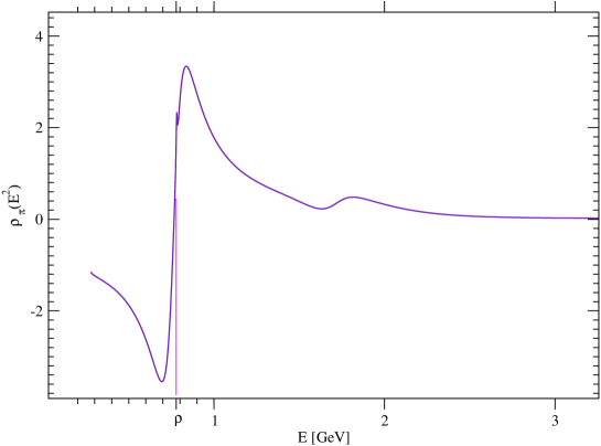
Figure 2: Spectral function of the pion electromagnetic form factor $F_{\pi}$. The peak for $\omega$ is visible slightly above $\rho$ meson mass, the later scale is indicated by the pointer and letter $\rho$. A naively expected spectral peak of the main $\rho$ resonance is distorted due to the presence of the background function $D_{bg}$.

Associated spectral function $\rho_{F}$ for the most likelihood (labeled AI) fit is shown in the Fig. 2 . Contrary to the vacuum polarization spectral function, the function $\rho_{F}$ is not positive definite. Requiring the positivity, we would get resonances more localized ( see the Tab. for small widths achieved), however the value of $\chi^{2}\simeq 6$ excludes this possibility as a reliable one. Interested reader can find fitted values in the table 1, where also parameters for the GS fit are shown for purpose of completeness. Although the meaning is lost, we still use the word “width” for various $\Gamma$ parameters used in associated fits.

fit	A I			A II	(constr)	G.S.	model
name	m	$\Gamma$	c	m	$\Gamma$	m	$\Gamma$
$\rho(775)$	778.48	146.379	-	780.02	152.3	773.25	148.6
$\omega$	781.684	8.4500	0.001514	781.69	8.53	780.4	9.609
$\rho(2)$	1202.0	1270.0	-0.0666	1299.0	150.0	—	—
$\rho(3)$	1694.0	704.00	-0.0666	1428.6	230.0	1356.5	252.2
$\rho(4)$	1735.0	291.7	0.0666	1742	134.0	1668	124.0
$\rho(5)$	2200.0	1242.0	-0.0666	2217	150.0	2217	320.0
$\chi^{2}$ /n.o.p.	1.0	/ 15 par.		6	/ 18 par.	1.6	/ 19 par.

Table 1: List of parameters for various fits as described in the text. AI stands for the most likelihood fit based on spectral representation, AII stands for the same but with with constrained positivity and G.S. stands for 19 parametric GS model. $\chi^{2}$ and number of free parameters are shown, $\chi^{2}$ functions are calculated with IE of AI for all fits for purpose of comparison. In order to avoid confusion a simple numbering is used to name the excited $\rho$ mesons.

All combined data and the most likelihood fit is shown in Fig. 1 (left panel) some details, e.g. chosen errors are shown in right panel of the Fig. 1. The constant phase in the Eq. (15) was fitted such that $\phi_{o}=-1.1303rad$, the overall normalization factor of the spectral function $\rho_{F}$ was found ${\cal{N}}^{-1}=0.85560$. Couplings for two additional fits are different, they are complex for GS fit and not displayed for brevity. Further details of GS fit are displayed in the Appendix.

To conclude this Section we argue that our 15 parametric analytical fit based on the spectral representation for the pionic form factor excellently describes the world combined data on two pions productions. Adding a new meson entity does not lead to substantial reduction of the inflated error. In implies, already right number of degrees freedom was achieved and the size of the IE is limited by property of the data rather then by quality of our fit.

V $\Pi_{h}$ determination

In the previous section we have found numerical fits for the most important contribution to HVP. The inflated error $\sigma_{I}(s)$ was determined by using the global $\chi^{2}$ criterion for each model fit separately. Form this point of view the 15 parameters spectral representation fit and 19 parameters GS model fit provided comparable good results, however their different analytical forms can lead to the local changes which are not completely clear from the global characteristic of $\chi^{2}$ fits. In order to see these effects we evaluate the muon production cross section and compare with precise measurement at phi meson peak as well as we compare electromagnetic running charge as has been measured by KLOE collaboration more recently.

Likewise in approaches polar2 ; polar3 ; DAVIER2011 , the method of obtaining of HVP herein is based on the integration of the Eq. (7), where in our case the smooth function $\sigma_{fit}$ is used for this purpose. In order to achieve our desired comparison one needs to add all remaining important contributions to $\sigma_{h}$. Following the similar routine as in the calculation of $\sigma_{\pi\pi}$ contribution, we have found fits with acceptably small continuous IE for the remaining exclusive channels: $K^{+}K^{-}$, $K_{L}K_{S}$ and $\pi\pi\pi$ as well as sub-dominant $\eta\gamma$ and $\pi\gamma$ production cross sections have been included. With the precision achieved the final states with four pions has been included as well, while we have neglected $KK\pi$ and the other states with higher multiplicity then 3. Neglected cross sections are flat, very small and their quantitative effect was estimated by comparison with off resonances HP functions calculated in polar2 ; polar3 , where these channels were recently included. Further, following the standard routine, the effect of well established vector charmonia and bottomonia has been included into $\sigma_{h}$ via their BW forms with PDG averaged values.

All necessary fits with sources of experimental data are described in the appendices, each separately devoted to the individual process as named above. For this purpose we profit from a number of accurate and compatible measurements as well as from a number of published well established and known interpolating fits for all necessary exclusive channels. For each case we however perform our own $\chi^{2}$ and determine IE. Fro the later, a using of formula (11) fully accepts the last experiments, eg. CMD-3, BESS-III, KLOE, as well as most SND,CMD-2 and BABAR measurements, while we have discard the data from old experiments (CMD,DM,NA7,OLYA,TOF). For each individual exclusive cross section we use just one fit, with the exception of the cross section $\sigma_{\pi\pi}$ discussed in preceding Section. All codes and required data inputs are collected at author’s web page www .

The second necessary ingredients to maintain precise comparison one needs to solve (7) with relatively high numerical precision. The so called Hollinde trick was used to perform principal value integration (for the meaning see for instance Eq. (C.2) in the paper SAULI2003 ). The integral equation (7) was solved iteratively within a combined integration methods (Simpson and Gaussian) at large numerical grid. In case of the use of the analytical fit for $\sigma_{\pi\pi}$ we have used the identical grid to evaluate the fit and the HVP. In this way we get rid of additional systematical numerical error due to the interpolation and have achieved numerical precision required for a meaningful comparison of tiny effects made by the use of different fits for $\sigma_{\pi\pi}$ cross section.

V.1 $\alpha_{QED}$ at $\phi$ meson energy

Let us start with the comparison of calculations for the muon pair productions at $\phi$ meson energy. HVP obtained by method described in previous Section and by other methods in polar2 ; polar3 is used to calculate $\mu\mu$ cross section and compared to the experiment in the Fig. 3. The line labeled by ”Th F.J.” or ”Th F.I.” represents cross section calculated with the use of HP in polar2 and in polar3 respectively.
-

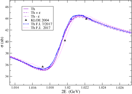
Figure 3: Muon pair cross section, comparison between theory and experiment as described in text.

Observed $\phi$-meson kick in $\mu\mu$ spectrum is reproduced by the Standard Theory dispersion relation and it is shown in the Fig.3. the error band (dashed and dot-dashed lines) is added.

The differences among various theoretical results have systematical origin due to the different strategy used for determination of HVP at $\phi$ meson invariant mass. Remind that the total error was governed by systematical error due to the luminosity and detection uncertainties ($\delta_{syst}=1.2\%$) all ”theoretical” lines agree with experiments within experimental errors. The error band (dashed and dot-dashed lines) is added into the figure for comparison as well. We do not show the error band for the calculation based on AI fit. Instead for purpose of figure we have used $c_{I}=0.8$ to determine the error band, recalling the fit based on the spectral representation for $\sigma_{\pi\pi}$ generates the same result at $\phi$ meson energy as the fit based entirely on $GS$ model. The figure is thus identical to those in SAHVP1 ; SAHVP2 . The KLOE data points are represented by triangles, noting that the standard statistical deviations roughly correspond with the size of the triangle. Slightly different situation appears at lower energy as it is discussed in the next Section.

VI $\alpha_{QED}$ at KLOE2

Very recently, the running of the electromagnetic coupling has been measured via radiative return method by KLOE2 collaboration KLOEdva . Thanks to achieved precision, it is for the first time, when the ”kick” effect was seen in the $\rho/$$\omega$ energy region. All calculated results for QED running coupling are compared in four figures, more specifically for the large region of $s$ in figures 4 as well as details for KLOE2 accessible region are shown for the left shoulder (left figure 5) and the right shoulder (right figure 5). All determined HP functions provide almost identical picture of the running coupling for KLOE2 energy region and there are very small difference between the result obtained here and in polar2 ; polar3 . A tiny error bands are not shown as they are about magnitude smaller then the standard experimental deviation.

In comparison to polar2 ; polar3 we have got a smaller polarization at very near of the muonic threshold. The origin of this remains unclear to the author. Looking elsewhere in momentum axis it should not originate in neglected high multiplicity final hadronic states (interested reader can find the portion of individual hadronic contributions for instance in SAHVP1 ; SAHVP2 ).

--

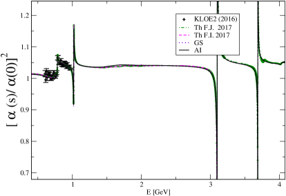
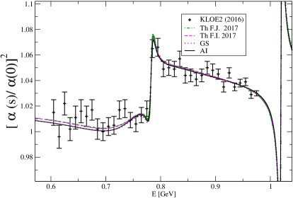
Figure 4: Square of the fine structure constant. Lines labeled by F.I. , F.J stand for HP extractions made by polar3 or polar2 respectively. Global view and comparison with KLOE2.

--

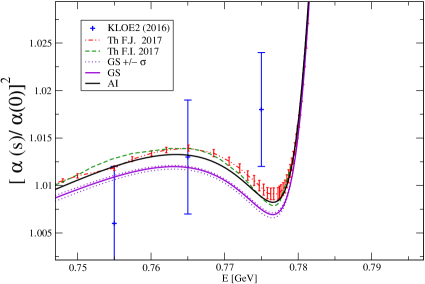
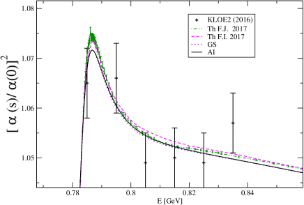
Figure 5: Square of the fine structure constant as in the previous figure. Details at the shoulders of $\rho/\omega$ peak.

VII Conclusion

The strategy of evaluation of HVP based on the use of fits for exclusive hadroproduction in $e^{+}e^{-}$ annihilation was suggested and the evaluation was performed in practice. We advocate for the use of special form for the inflated error which mix statistical and systematic errors of several experiments and is particularly suited for the analyzes of combined data on $\sigma_{h}$ bellow $3GeV$. In addition to some popular phenomenological fits, the dispersion relation for the pion electromagnetic form factor was found to be excellently working here. Within a reduced number of free parameters describing the form factor, it provides best fit for combined data from the threshold $2m_{\pi}$ to 2.5 GeV. However it turns that some of identified resonances, including also reintroduced excited meson $\rho(1250)$, are largely affected by presence of the background as well as their mutual interference is enhanced and plays the role. Nevertheless, the entire spectral function $\rho_{\pi}$ is considerably simple and can be used to evaluate other physical quantities (e.g. anomalous magnetic moments of leptons).

The aforementioned spectral fit together with the other considered fits for $\pi\pi$ (hadronic) production cross sections have been then utilized to calculate of $\sigma_{\mu\mu}$ cross section and QED running charge at the timelike region of momenta and compared with 2004 KLOE $\sigma_{\mu\mu}$ as well ass with 2016 KLOE2 measurement for the electromagnetic running charge. In both cases the “theoretical” error due to the determined inflated error of $\sigma_{h}$ was shown to be several times smaller then the total experimental errors. Obtained results have been compared with those where hadronic vacuum polarization was extracted by other methods. Based on the mutual comparison of different fits of $\sigma_{h}$, which have the similar global quality quantified by $\chi^{2}$, allowed us to show that (difficult to estimate) systematical error due to the methodology used herein is reasonable small.

Regarding our best resulting fit for the process $\sigma_{\pi\pi}$, the masses of $\rho(n)$ relatively agree with the others (rupp ), whilst widths are much larger in case of two first excited states. The reason is that there is a relatively admixture with the background functions $D_{bg}$, which enhance the mutual interference among resonances as well. Obviously, the overlap of resonances is such enormous, that the interpretation of such contributions as radially excited mesons can be a severe simplification of more complicated nonperturbative terms. To this point let us mention the observation sauli2020 , where it was shown that the quark dynamical mass function is not a smooth function of momentum variable at the timelike region and no simple quantum mechanical model, which uses a constant quark mass approximation, can be therefore reliable trusted. Actually, the running of masses at the timelike region can cause reordering or mutual washout of resonances and $\rho(2)$ and $\rho(3)$ vectors are not distinguishable in principle. Due to the same reasoning the mass of $m_{K}^{*}$ does not need to be heavier then $m_{\rho(2)}$ if one needs to avoid very large meson width for any reason. In a honest approach, a wide resonances can be regarded as an effective description of more non-perturbative contributions mixtured at once.

VIII Acknowledgments

The author is grateful to P. Bydžovský for stimulating discussions and thanks to prof. F. Jagerlehner for his help and advice to run the code polar2 and to G. Venanzoni for invitation to FCCP 2017, which was partially motivating and useful for final comparisons with the data of other groups.

Appendix A Details on analytical fit

In this appendix we review the list of functions, which have been used in our constructions.

Especially important is the form of Gounaris-Sakurai dressed vector meson propagator, which reads

$${\cal W}^{GS}=\frac{m^{2}+d(m)\Gamma/m}{M^{2}(s)-s-im\Gamma(s,m,\Gamma)}\,\,,$$ (16)

$$M^{2}(s)=m^{2}\left[1+\frac{\Gamma k^{2}(s)}{k^{3}(m)}(h(s)-h(m^{2}))+\frac{\Gamma h^{{}^{\prime}}(m^{2})}{k(m)}(m^{2}-s)\right]\,\,,$$ (17)

$$\Gamma(s,m,\Gamma) = \Gamma\frac{m}{\sqrt{s}}\left[\frac{L_{2}(s,m_{\pi})}{L_{2}(m^{2},m_{\pi})}\right]^{3}\,\,,$$

$$L_{2}(s,m_{\pi}) = \sqrt{s-4m^{2}_{\pi}}\,\,,$$ (18)

where we have defined following auxiliary functions:

$$h(s)=\frac{\beta(s)}{2}\ln\left(\frac{\sqrt{s}+2k(s)}{2m_{\pi}}\right)\,\,,$$ (19)

$$h^{{}^{\prime}}(m^{2})=\frac{2m_{\pi}^{2}h(m)}{m^{4}\beta(m)}+\frac{2m_{\pi}^{2}}{\pi m^{4}\beta(m)}+\frac{\beta(m)}{2\pi m^{2}}\,\,,$$ (20)

$$d(m)=\frac{4m_{\pi}^{2}}{m^{2}\beta^{3}(m)}(3h(m)-2/\pi)+\frac{1}{\pi\beta(m)}\,,$$ (21)

with the usual shorthand notation:

$$\beta(s)=\frac{L_{2}(s,m_{\pi})}{\sqrt{s}}\,\,,\,\,k(s)=\frac{L_{2}(s,m_{\pi})}{2}\,\,,$$ (22)

used for the velocity and the two pion Lorentz invariant phase space factor.

The Breight-Wigner function for the narrow $\omega$ meson was taken in the form:

$${\cal W}_{\omega}=\frac{m^{2}_{\omega}}{m^{2}_{\omega}-s-im_{\omega}\Gamma_{\omega}}\,.$$ (23)

Appendix B Gounaris-Sakurai fit of $F_{\pi}$

The G-S fit for combined data reads

$$F_{GS}(s)=\frac{{\cal W}^{GS}_{\rho}(s,m_{\rho},\Gamma_{\rho}){\cal D}_{\rho}(s)\frac{1+c_{\omega}{\cal W}_{\omega}(s,m_{\omega})}{1+c_{\omega}}+\sum_{i}c_{\rho^{i}}{\cal W}^{GS}_{\rho^{i}}(s,m_{\rho^{i}},\Gamma_{\rho^{i}})}{1+c_{\rho^{1}}+c_{\rho^{2}}+c_{\rho^{3}}}\,\,.$$ (24)

where the entering functions ${\cal W}^{GS}$ and ${\cal W}_{\omega}$ are identical to those defined in the previous appendix. However here they are taken with complex prefactors: $c_{V}=|c_{V}|e^{i\phi_{V}}$. In addition we have found advantageous to deform $\rho/\omega$ peak by the introduction of auxiliary function ${\cal D}_{\rho}$, which was chosen such that ${\cal D}_{\rho}=1$ above $\rho$ meson mass and

$${\cal D}_{\rho}(s)=x+(1-x)\left[\frac{1-4m_{\pi}^{2}/s}{1-4m_{\pi}^{2}/m_{\rho}^{2}}\right]^{1/2}\,,$$ (25)

bellow the value $s=m_{\rho}^{2}$. The parameter $x$ was fitted providing the value $x=0.37202$.

The index i runs over the resonances labeled as $\rho(1500)$, 2 for$\rho(1800)$ and $i=3$ stands for BaBar resonance corresponding with the peak at $2200MeV$ in the paper SAHVP2 , while they are relabeled for purpose of this paper as $\rho(3),\rho(4)$ and $\rho(5)$ respectively.

Appendix C Fit for $\pi^{+}\pi^{-}\pi^{0}$ channel

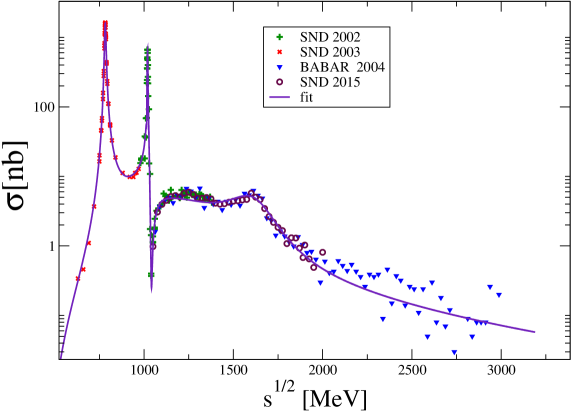
Figure 6: Measured $\sigma_{3\pi}$ and the fit, global view.

Complicated by the shape, $e^{+}e^{-}\to 3\pi$ total cross section consists from two dominant peaks of the narrow omega and phi vector resonance. The first peak can be represented by an almost perfect BW function, while the second one is crudely deformed as the $\phi$ meson peak turns abruptly down and makes the fitting more complicated. Happily a sum of complexified and slightly deformed BW functions provide very good auxiliary function for making a fit out of the data even without taking of full correct three pions phase space and without the use of any ”background function”. However these are the data itself which does not allow to minimize $\chi^{2}$ with the same error function as in the previous case and the IEF is taken slightly larger by enlarging the coefficients in Eq. (11) such that $c_{L}=1nb^{1/2}$ and $c_{s}=1$ . In this exceptional case we get minimized $\chi^{2}$ slightly larger then one: $\chi^{2}=1.23$ with the resulting curve and the data shown in the Fig. 6 and in the Fig. 7 in detail. Note also here, that we get $\chi^{2}=0.95$ if we cut the data above $1.05GeV$, having thus the region of $\omega$ and $\phi$ mesons under a better control.

Like in the previous case, only BW functions with masses higher then the threshold are used. We do not exploit VMD idea of rho meson as an intermediator, wherein virtual decay $\omega\rightarrow\pi\rho\rightarrow 3\pi$ would require ”dressed” rho meson propagator and numerical integration over the three body phase space would be needed. This would inevitably causes a drastic grow of the time of the minimization procedure (from days to unacceptable years). Actually, we are not improving a given VMD model but we are looking for the smallest $\chi^{2}$ instead, for which purpose the use of proposed auxiliary functions is more suited in practice.

Our simplified fit therefore reads:

$$\sigma_{3\pi}(s) = \frac{12\pi}{s^{3}}L_{3}(s)\left|\sum_{V=\omega,\phi}{\cal W}_{V}{\cal D}_{V}+\sum_{V=1,2,3}{\cal W}_{V}\right|^{2}\,\,,$$

$${\cal W}_{V} = \frac{m_{V}\Gamma_{V}(s)e^{i\phi_{V}}}{m_{V}^{2}-s-im_{V}\Gamma_{V}(s)}\sqrt{\frac{m_{V}B_{V}}{L_{3}(m_{V}^{2})^{3}}}\,\,,$$ (26)

where for all $V$ the auxiliary functions now read

$$\Gamma_{V}(s) = \Gamma_{V}\frac{m_{V}L_{3}^{3}(s)}{s^{1/2}L_{3}^{3}(m_{V}^{2})}\,,$$

$$L_{3}(s) = \sqrt{s-9m_{\pi}^{2}}\,,$$ (27)

and where the function which further deform omega meson peak reads

$${\cal D}_{\omega}(s) = \left[1+c_{1}\frac{s-m_{\omega}^{2}}{2}+c_{2}\sqrt{s-m_{\omega}^{2}}\right]^{-1}\Theta(s-m_{\omega}^{2})+$$ (28)

$$+ \left[1+c_{3}\frac{(s-m_{\omega}^{2})}{2}+c_{4}\sqrt{m_{\omega}^{2}-s}\right]^{-1}\Theta(m_{\omega}^{2}-s)\,\,,$$

with fitted constants $c_{1}=0.105321{\mbox{G}eV}^{-2}$, $c_{2}=-0.0598{\mbox{G}eV}^{-1}$, $c_{3}=-0.254221{\mbox{G}eV}^{-2}$, $c_{4}=0.055406{\mbox{G}eV}^{-1}$.

Whilst the function which deforms BW shape of $\phi$ meson is chosen different from $\omega$ and reads

$${\cal D}_{\phi}(s)=1+{\cal W}_{L}(s)\Theta(m^{2}_{\phi}-s)+{\cal W}_{R}(s)\Theta(-m^{2}_{\phi}+s)\,,$$ (29)

where in Eq. (29) BW functions (26) are taken. Stress here, that these functions serve to deform the shape of the left and the right shoulder of $\phi$ meson resonance and they appear in the product with $\phi$ meson BW and should not be confused with a conventional meson. All fitted numbers are listed in Tab. (2). In the function $L_{3}$ the value $m_{\pi}=139.57018{\mbox{M}eV}$ is taken, ignoring the difference between charged and neutral pion mass. The cross section is taken from $\sqrt{s}=3m_{\pi}$, bellow it is zero.

–	mass/MeV	width/MeV	B	$z$
$\omega$	782.6141	8.7031	$3.0885\,\,10^{-5}$	0
L	1015.461	2.813	0.167	134.1
R	1025.487	12.301	0.121	184.35
$\phi$	1019.704	4.067	$5.0807\,\,10^{-5}$	163.62
$V_{1}$	1086.425	252.0	$8.9\,\,10^{-7}$	124.36
$V_{2}$	1219.280	569.0	$2.97\,\,10^{-7}$	78.123
$V_{3}$	1636.32	278.0	$1.52\,\,10^{-6}$	174.62

Table 2: Parameters of the cross section fit for $\sigma_{K^{+}K^{-}}$ as described in the text.

In usual VMD’s the parameter $B$ stands for the product of branch ratios $Br(V\to ee)Br(V\to 3\pi)$. Here the value for $\omega$ meson significantly differs from the BaBaR measurement ($Br(\omega\to ee)Br(\omega\to 3\pi)_{\mbox{B}aBaR}=6.7\,\,10^{-5}$) since the fit is different as well. There are other differences, whether stemming from our different formula for the fit is not obvious. The last resonance agrees with the meson conventionally labeled as $\omega^{{}^{\prime\prime}}$ (see 3piSND2015 ), noting also that $\phi^{{}^{\prime}}$ observed at the same energy in other process (see the next Section) should be there as well. On the other side, there is no good evidence for super-wide ($\Gamma\simeq 900MeV$) SND/BaBaR established meson. This, over all overlapping resonance, conventionally labeled $\omega^{{}^{\prime}}$, with quoted mass $\simeq 1470\pm 50$ by SND2015, is preferably replaced by two BW functions with much lower masses and different complex couplings. Of course, recalling the meaning and purpose of our fit, which uses complex phases and avoids a use of correct 3-body phase space, does not allow to make a strong statement about the vector meson content of $\sigma_{3\pi}$ cross section.

-

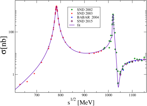
Figure 7: Selected data for $\sigma_{3\pi}$ and the fit, view on the peaks.

Appendix D Fit for cross section of the process $e^{+}e^{-}\to K^{+}K^{-}$

Very important, since the most dominant exclusive process at $\phi$ meson peak energy, has been measured not only on the peak, but thanks to the ISR method also fairly above: up to the total energy $E=8{\mbox{G}eV}$. Fine selected data are chosen from several last measurements, e.g. the most precise data charcmd2 are fully taken into account, we have also used selection survived (off peak) data as obtained by SND chargeSND1 ; chargeSND2 , and from the energy 1350 MeV till 5 GeV we exploit the BaBaR data chargebababar1 ; chargebababar2 , providing total $N_{d.o.f}=142$ for $K^{+}K^{-}$ cross section. Remind two important notes here for completeness. Firstly, the $J/\Psi$ and $\Psi^{\prime}$ peaks were subtracted by BaBaR collaboration and we add them separately. Secondly, keeping a certain amount of threshold BaBaR data is possible, in a way one still keeps $\chi^{2}<1$ without changing fit. Here we simply preferred to keep $\chi^{2}$ lower, with $N_{d.o.f.}$ smaller for future purposes. Fit for the charged K meson pair production cross section reads

$$\sigma_{K^{+}K^{-}}(s)=|A|^{2}s^{-5/2}f_{c}\left[\frac{L_{2}(s,m_{K})}{L_{2}(m_{\phi}^{2},m_{K})}\right]^{3}$$ (30)

with the function $f_{c}$ in used is defined as

$$f_{c} = \frac{1+\alpha\pi(1+v(s)^{2})/2v(s)}{1+\alpha\pi(1+v(m_{\phi}^{2})^{2})/2v(m_{\phi}^{2})}\,\,,$$

$$v(s) = L_{2}(s,m_{K})/\sqrt{s}\,\,,$$ (31)

where $m_{K}$ is the mass of charged Kaon, $L_{2}$ is defined earlier in (18), and the amplitude is given by the sum of $BW$ functions:

$$A=\sum_{V}e^{iz_{V}}{\cal W}_{V}(s)=\sum_{V}e^{iz_{V}}\frac{\sqrt{c\,m_{V}\,B_{V}\,\Gamma_{V}}}{m^{2}_{V}-s-i\Gamma_{V}\sqrt{s}}\,\,,$$ (32)

where $c=4.5465\,\,10^{-5}$, and where all BW functions are common for narrow as well as for wide resonances.

The sum in (32) runs over the BW functions, noting that the four of lowest five can be identified with usual i.e. more or less established radial excitation of the $\phi$ and $\omega$ . Their names are quoted in bracket in the first column of the Tab. 3. The one unlabeled there has a small coupling to the leptons and do not need to be necessarily related with conventional meson, however it helps to accommodate the shape of fit to the cross section data. Up to the ground state meson, we are not strongly pointing a given BW structure with a given meson name, since due to the interference effect the parameters are strongly correlated. In general, it is hard to label overlapping resonances, noting trivially that the observed pattern above $\phi$ meson arises from the admixture of the light flavor quark-antiquark components, however what is flavor content of a single broad BW peak is not obvious, at least when comparing to electrically neutral ground state vectors: $\phi,\omega$ and $\rho$ mesons. Selected data and the fit with $\chi^{2}=0.56$ (obtained with IEF) are illustrated at Fig. 8.

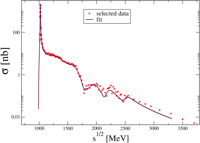
Figure 8: Selected data for $\sigma_{K^{+}K^{-}}$ and the fit, $\phi$ peak view.

label(content)	mass/MeV	width/MeV	B	$z$
$\phi$	1019.2469	4.1358	0.5377	0
$V_{1}(\omega^{{}^{\prime}})$	1337.1	372.83	0.00890	180.71
$V_{2}(\phi^{{}^{\prime}}\omega^{{}^{\prime\prime}})$	1624.8	307.406	0.0061	222.53
-	1813.033	80.01	0.0003535	92.6
$V_{3}(\phi^{{}^{\prime\prime}})$	1892.36	262.0	0.00252	104.91
$V_{4}$	2178	157.7	0.000175	100.2
$V_{5}$	2510	160.1	0.0000364	134.2

Table 3: Numbers for charged kaons channel

Appendix E Fit for the neutral kaons channel $e^{+}e^{-}\to K^{0}_{S}K^{0}_{L}$

-

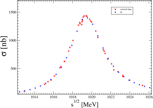
Figure 9: Measured $\sigma_{K_{L}K_{S}}$ and the fit around the peak position.

To fit the process $\sigma(e^{+}e^{-}\to K^{0}_{S}K^{0}_{L})$ we have used the data collected by Novosibirsk SND,CMD-2 collaborations and very newly by CMD-3 group SNDKK2001 ; CMD2KK2004 ; CMD3KK2016 as well as the BaBaR data BABARKK2014 were exploited above $\phi$ meson peak. For this purpose the similar formula as for the process $e^{+}e^{-}-->K^{+}K^{-}$ is used, however in addition to that, we have introduced the deformation function into the cross section (i.e. there is a change $|A|^{2}\rightarrow d(s)|A|^{2}$), where the function $d$ is represented by the following step functions

$$d(s) = \left[1+\frac{d_{1}(s-m_{\phi}^{2})}{2}+d_{2}\sqrt{s-m_{\phi}^{2}}\right]^{-1}\Theta(s-m_{\phi}^{2})$$ (33)

$$+ \left[1-\frac{d_{3}(s-m_{\phi}^{2})}{2}-d_{4}\sqrt{m_{\phi}^{2}-s}\right]^{-1}\Theta(m_{\phi}^{2}-s)$$

and four fitted numbers within four(five) digit accuracy read: $d_{1}=1.3204{\mbox{G}eV}^{-2},d_{2}=0.8615{\mbox{G}eV}^{-1},d_{3}=12.371{\mbox{G}eV}^{-2},d_{4}=1.291{\mbox{G}eV}^{-1}$.

The amplitude is made out solely from BW functions, wherein we have found that three vector mesons are enough. However, due to the flatness of the cross section, it is advantageous to distinguish the narrow $\phi$ meson and wide resonances. The appropriate BW functions read:

$${\cal W}_{\phi}(s) = \frac{m_{\phi}^{3}\sqrt{12\pi\Gamma_{\phi}B_{\phi}/m_{\phi}}}{m^{2}_{\phi}-s-i\Gamma_{\phi}\frac{s}{m_{\phi}}}\,\,,$$

$${\cal W}_{V}(s) = e^{iz_{V}}\frac{m_{V}\Gamma(s,m_{V})\sqrt{B_{V}m_{V}/L_{3}(m_{V}^{2},m_{\pi})}}{m^{2}-s-im_{V}\Gamma(s,m_{V})}\,\,,$$

$$\Gamma(s,m_{V}) = \frac{m_{V}\Gamma_{V}}{\sqrt{s}}\left[\frac{L_{3}(s,m_{\pi})}{L_{3}(m_{V}^{2},m_{\pi})}\right]^{3}\,\,,$$ (34)

where we have used $L_{3}$ function for the running width for resonances $V_{1}\simeq\phi^{,}$ and $V_{2}\simeq\phi^{,,}$. Relevant numbers are listed in the Tab. 4 :

	mass/MeV	width/MeV	B	$z$
$\phi$	1019.3886	4.2612	$0.4235\,10^{-6}$	–
$V_{1}$	1670.320	198.0	$0.24975\,10^{-6}$	177.5
$V_{2}$	2066.985	248.5	$0.3072\,10^{-6}$	147.8

Table 4: Numbers for neutral kaons channel

To get the fit the data with $N_{d.o.f}=93$ has been used. The results are sketched in figures 9 and 10.

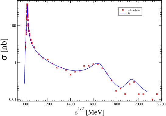
Figure 10: Measured $\sigma_{K_{L}K_{S}}$ and the fit, global view.

Appendix F Fit for the $\eta\gamma$ and $\pi\gamma$ cross sections

-
-

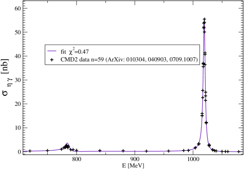
Figure 11: Measured $\sigma_{\eta\gamma}$ and its fit.

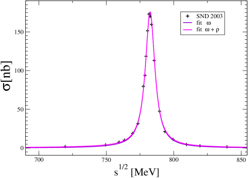
Figure 12: Measured $\sigma_{\pi\gamma}$ and two fits as described in the text are shown.

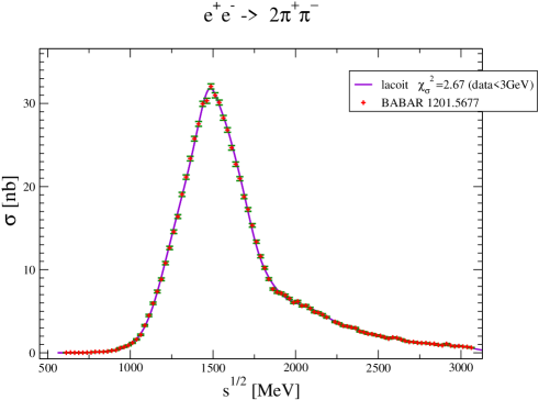
Figure 13: Measured $\sigma_{4\pi}$ and the fit.

The fit of the cross section of the process $e^{+}e^{-}\to\pi^{0}\gamma$ is based on simple admixture of $\rho$ and $\omega$ BW functions with constant parameters. It reads

$$\sigma_{\pi\gamma}(s)=K(1-m_{\pi}^{2}/s)^{3/2}\left[\frac{m_{\omega}^{4}}{(m_{\omega}^{2}-s)^{2}+\Gamma_{\omega}^{2}m_{\omega}^{2}}+2.1\frac{m_{\rho}^{4}}{(m_{\rho}^{2}-s)^{2}+\Gamma_{\rho}^{2}m_{\rho}^{2}}\right]$$ (35)

with $K=64/(3m_{\pi}^{2})10^{-9}$ and the remaining parameters are $m_{\omega}=782.5MeV,\Gamma_{\omega}=8.63MeV;m_{\rho}=775.02MeV,\Gamma_{\rho}=149.59MeV$. We neglect the interference term in this case. The resulting fit is shown in the Fig. 12 where also the fit with only $\omega$ meson is shown for interesting comparison (numbers not shown). The better fit, the one with inclusion of $\rho$ meson, is used for the calculation of hadronic $\Pi_{h}$.

For the cross section $\sigma_{\eta\gamma}$ we have used the data with $N_{d.o.f}=59$ measured by CMD-2/SND detectors and published in the period 2001-2014 etagam1 ; etagam2 ; etagam3 , where also the data for $\sigma_{\pi\gamma}$ has been obtained.

The parameterization of the cross section was chosen such that

$$\sigma_{\eta,\gamma}(s)=\frac{1}{s}\left[{\cal W}_{\omega}(s,m_{\omega})+e^{iz_{\phi}}{\cal W}_{\phi}(s,m_{\phi}){\cal D}(s)\right]^{2}\,\,,$$ (36)

where the choice (32) for BW was made. Only $\omega$ and $\phi$ mesons are considered and heavier mesons are ignored as the cross section for $\eta,\gamma$ production is fairly small etagam3 at higher energies. The deformation is considered for the $\phi$ meson case, while the phase space factor is effectively absorbed into the fit.

The fitted values of BW parameters are $m_{\omega}=785.9MeV,\Gamma_{\omega}=9.06MeV;m_{\phi}=1019.415MeV,\Gamma_{\rho}=4.0306MeV$ and the deformation function is chosen as

$${\cal D}(s) = \left[1+\frac{24.49GeV^{-2}(s-m^{2})}{2}+0.1326GeV^{-1}\sqrt{s-m_{\phi}^{2}}\right]^{-1}\Theta(s-m_{\phi}^{2})+$$ (37)

$$+ \left[1+\frac{-4.62GeV^{-2}(s-m2)}{2}-3.0GeV^{-1}\sqrt{m_{\phi}^{2}-s}\right]^{-1}\Theta(m_{\phi}^{2}-s)\,\,.$$

The phase was fitted such that $z_{\phi}=20.65^{o}$. The fitted function and the data are shown in the Fig. 11.

Appendix G Fit for the $4\pi$ cross section

To fit the cross section $\sigma(e^{+}e^{-}\to 4\pi)$ we used the data collected by BaBaR collaboration ctyripi . Working with single measurement the experimental statistical error can be used to find a fit, in this case $\chi^{2}=2.7$ was achieved, providing safe constrain $\chi^{2}<1$ when IEF is used instead. As a fitting function we have chosen the product of two BW’s series with a suitable phase factor. It simulates $2\rho$ peak with other six heavy excitation in combination included as well. Further, the shape is modified by the function made out of the sum of unit and the eight properly centered Gaussian functions. Like in previous case, the fit serves for numeric and should not confused with any ”effective theory” calculation and it should be regarded as such. We do not write down the full details of the fit, noting only here, it involves 28 parameters related with BW functions and their mixing, and 24 parameters related with Gaussian functions (for interested reader, the code can be sent via email on request of the author). The number of parameters are not used to reduce n.d.f. (number of data points). The fitted function and the data are shown in the Fig. 13.

References

- (1) G. Bennet et al., Phys. Rev. Lett. 89, 101804 (2002).
- (2) K. Olive et al., Rewiev of Particle Physics, The Muon Anomalous Magnetic Moment by A. Hoecker and B. Marciano, Chin. Phys. C 38, 090001 (2014).
- (3) B. Abi et al., Phys. Rev. Lett. 126, 141801 (2021).
- (4) J. E. Augustin, et al.; Phys. Rev. Lett. 30, 462 (1973).
- (5) F. A. Berends and G.J. Komen, Nuc. Phys. B 115, 114-140 (1976).
- (6) F. Ambrosino, et al.; Phys. Lett. B 608, 199-205 (2005).
- (7) F. Jegerlehner, J. Phys. G 29, 101 (2003), the updated code is available at http://www-com.physik.hu-berlin.de/ fjeger
- (8) The vacuum polarisation corrections used by Novosibirsk experiments (SND, CMD2, CMD3): http://cmd.inp.nsk.su/ ignatov/vpl .
- (9) KLOE2 Collab. and F . Jegerlehner, Phys. Lett. B 767, 485–492 (2017).
- (10) N. Hammoud, R. Kamiński, V. Nazari, G. Rupp, Phys. Rev. D 102, 054029 (2020).
- (11) T. Hilger, M. Gomez-Rocha, A. Krassnigg, Eur. Phys. J. C 77, 625 (2017).
- (12) T. Goecke, Ch. S. Fischer, R. Williams, Phys. Lett. B 704, 2011-217 (2011).
- (13) V. Sauli, Few Body Syst. 61 , 3, 23 (2020).
- (14) A. B. Arbuzov, et al.; JHEP 9710, 001 (1997).
- (15) N. Cabibbo and R. Gatto, Phys. Rev. 224, N.5,1577-1595 (1961).
- (16) S. Eidelman, F. Jegerlehner, Z. Phys. C67, 585-602 (1995).
- (17) M. Davier, A. Hoecker, B. Malaescu, Z. Zhang, Eur. Phys. J. C71, 1515 (2011).
- (18) P. Bydzovsky, R. Kaminski, and V. Nazari, Phys. Rev. D 94, 116013 (2016).
- (19) E. Bartos, S. Dubnicka, A. Liptaj, A. Z. Dubnickova, and R. Kaminski, Phys. Rev. D 96, 113004 (2017).
- (20) V.Sauli, Acta Phys. Polon .Supp. 10 no.4, 1159-1164 (2017).
- (21) V. Sauli, ArXiv:1708.03616, EPJ Web Conf. 179, 01021 (2018).
- (22) M. Hoferichter, P. Stoffer, JHEP 1907, 073 (2019).
- (23) K. Hagiwara, R. Liao, A.D. Martin, Daisuke Nomura, T. Teubner, J. Phys. G38, 085003 (2011);
- (24) A. Anastasi et al., Phys.Lett. B767 485 (2017).
- (25) V. Sauli, JHEP 0302, 001 (2003).
- (26) A. Aloisio, et al (KLOE Collaboration), Phys. Lett. B 606, 12–24 (2005).
- (27) V. M. Aulchenko, et al (CMD-2 Collaboration), JETP Lett. 82, 743-747 (2005); PismaZh. Eksp. Teor. Fiz. 82, 841-845 (2005).
- (28) M.N.Achasov,et al, J. Exp. Theor. Phys. 103, 380-384 (2006); Zh. Eksp. Teor. Fiz. 130, 437-441 (2006).
- (29) J. P. Lees (BABAR Collaboration), Phys. Rev. D 86, 032013 (2012).
- (30) M. Ablikim, (BESIII Collaboration) Phys. Lett. B753, 629-638 (2016).
- (31) E.L. Lomon, S. Pacetti, Analytic pion form factor, arXiv:1603.09527
- (32) G. J. Gounaris and J. J. Sakurai, Phys. Rev. Lett. 21, 244 (1968).
- (33) R. R. Akhmetshin et al (CMD-2 Collaboration), Phys. Lett. B578, 285-289 (2004).
- (34) M. N. Achasov et al, Phys. Rev. D 68, 052006 (2003).
- (35) M.N.Achasov et al, Phys. Rev. D66, 032001 (2002).
- (36) V. M. Aulchenko et al,JETP, 121, 27–34 (2015).
- (37) B. Aubert, et al (The BABAR Collaboration), Phys. Rev. D70, 072004 (2004).
- (38) R.R.Akhmetshin (CMD-2 collaboration), Phys. Lett. B669, 217-222 (2008). R.R.Akhmetshin et all., Phys. Lett. B695, 412-418 (2011).
- (39) M. N. Achasov et al., Phys. Rev. D63, 072002.
- (40) M. N. Achasov et al. (SND Collaboration), Phys. Rev. D 76, 072012 (2007).
- (41) The BABAR Collaboration,Phys. Rev. D 88, 032013 (2013).
- (42) The BABAR Collaboration, Phys. Rev. D 92, 072008 (2015).
- (43) M.N, Achasov, Phys. Rev. D63, 072002 (2001).
- (44) R. R. Akhmetshin (CMD-2 collaboration), Phys. Lett. B578, 285-289 (2004).
- (45) E. A. Kozyrev (CMD-3 collaboration), Phys. Lett. B 760, 10, 314-319 (2016); E. A. Kozyrev (CMD-3 collaboration), PHIPSI15, ArXiv:1603.03230.
- (46) The BABAR Collaboration, J. P. Lees, Phys. Rev. D 89, 092002 (2014).
- (47) CMD-2 collab., Phys. Lett. B509, 217-226 (2001).
- (48) M. N. Achasov, Phys. Rev. D76, 077101 (2007).
- (49) M. N. Achasov, et al. Phys. Rev. D 90, 032002 (2014).
- (50) The BABAR Collaboration, J. P. Lees, Phys. Rev. D 85, 112009 (2012).
- (51) Most important codes and data files are usualy stored at the athor’s web page: http://gemma.ujf.cas.cz/ sauli/papers.html