Formation Control and Network Localization via Distributed Global Orientation Estimation in $3$-D

Abstract

In this paper, we propose a novel distributed formation control strategy, which is based on the measurements of relative position of neighbors, with global orientation estimation in 3-dimensional space. Since agents do not share a common reference frame, orientations of the local reference frame are not aligned with each other. Under the orientation estimation law, a rotation matrix that identifies orientation of local frame with respect to a common frame is obtained by auxiliary variables. The proposed strategy includes a combination of global orientation estimation and formation control law. Since orientation of each agent is estimated in the global sense, formation control strategy ensures that the formation globally exponentially converges to the desired formation in 3-dimensional space.

I Introduction

Cooperative control of multiple autonomous agents has attracted a lot of attention due to its practical potential in various applications. Formation control of mobile autonomous agents is one of the most actively studied topics in distributed multi-agent systems. Depending on the sensing capability and controlled variables, various problems for the formation control have been studied in the literature [1].

Consensus-based control law for the desired formation shape is known as the displacement-based approaches. In this approach, agents measure the relative positions of their neighbors with respect to a common reference frame. Then, agents control the relative position for the desired formation. In the literature, it has been known that this method achieves global asymptotic convergence of the formation to the desired one [2, 3, 4, 5]. Fundamental requirement for the displacement-based approach is that all agents share a common sense of orientation. Therefore, local reference frames need to be aligned with each other. Oh and Ahn [5] found the displacement-style formation control strategies based on orientation estimation, under the distance-based setup (i.e., local reference frames are not aligned with each other). In this approach, agents are allowed to align the orientation of their local coordinate systems by exchanging their relative bearing measurements. By controlling orientations to be aligned, the proposed formation control law allows agent to control relative positions simultaneously. Similar strategy using the consensus protocol is found in [6]. In the paper, control objective is to reach a desired formation with specified relative positions and orientations in the absences of a global reference frame. These strategies ensure asymptotic convergence of the agents to the desired formation under the assumption that interaction graph is uniformly connected and initial orientations belong to an open interval $[0,\pi)$[5, 6]. In our previous work[7], we proposed a novel formation control strategy via the global orientation estimation. The orientation of each agent is estimated based on the relative angle measurement and auxiliary variables assigned in the complex plane. Unlike the result of [5, 6], in this new approach, consensus property, which is based on the Laplacian matrix with complex adjacency matrix, is applied to allow the global convergence of the auxiliary variables to the desired points. In this way, we showed that the global convergence of formation to desired one for the multi-agent system having misaligned frames could be achieved.

In this paper, we extend the result of [7] to 3-dimensional space. Even though we share the philosophy of the algorithm of [7], there are intrinsic distinctions from [7] as follows. First, in 2-dimensional space, an unique auxiliary variable for each agent is required to estimate the orientation of the local frame. However, for the estimation of orientation in 3-dimensional system, we require more than two auxiliary variables for each agent, since at least two auxiliary variables are required for obtaining the rotation matrix in $\mathrm{SO}(3)$. Second, while the direction of the unique auxiliary variable can be considered as the orientation in 2-dimensional space, the orientation in 3-dimensional space can not be determined directly from the two different directions of auxiliary variables. Thus, we need to have additional processes compared to the case of 2-dimensional space for obtaining the estimated orientation. The novel method proposed in this paper uses the consensus protocol with auxiliary variables to estimate a rotation matrix in $\mathrm{SO}(3)$. This consensus protocol achieves global convergence of auxiliary variable, since configuration space of auxiliary variable is a vector space instead of nonlinear space like circle. We show that auxiliary variables construct the rotation matrix that identifies the estimated orientation. For the case of general $n$-dimensional space, the estimation method for unknown orientation is proposed in our previous work[8]. In this paper, we modify the estimation method for the case of 3-dimensional space, and combine it with the formation control law for the desired formation shape. The estimated direction of the frame is used to compensate misaligned frames of each agent in the formation system. Consequently, the formation control law with the estimated coordinate frame achieves a global convergence of multi-agent system to desired shape in 3-dimensional space, under the distance-based setup. Third, we also show that the proposed strategy can be applied to the localization problem of sensor networks equipped with displacement and orientation measurement sensors. We design the position estimation law for the given displacement measurements. Then, the position estimation law is combined with the orientation estimation law. It thus shows that convergence property of localization algorithm is identical to the one of formation control algorithm.

The outline of this paper is summarized as follows. In Section II, preliminaries are described. In Section III, an idea for estimation law is described and stability of estimation law is analyzed. Convergence property of the formation control strategy with orientation estimation is then analyzed in Section IV. By using the proposed method, localization algorithm in networked systems is analyzed in Section V. Simulation results are provided in Section VI. Concluding remarks are stated in Section VII.

II Preliminaries

In this paper, we use the following notation. Given $N$ column vectors $x_{1}$, $x_{2}\dots x_{N}\in\mathbb{R}^{n}$, $\mathbb{x}$ denotes the stacking of the vectors, i.e. $\mathbb{x}=(x_{1},x_{2},\dots,x_{N})$. The matrix $I_{n}$ denotes the $n$-dimensional identity matrix. Given two matrices $A$ and $B$, $A\otimes B$ denotes the Kronecker product of the matrices. The exterior product, also known as wedge product, of two vectors $u$ and $v$ is denoted by $u\wedge v$.

II-A Consensus Property

Given a set of interconnected systems, the interaction topology can be modeled by a directed weighted graph $\mathcal{G}=(\mathcal{V},\mathcal{E},\mathcal{A})$, where $\mathcal{V}$ and $\mathcal{E}$ denote the set of vertices and edges, respectively, and $\mathcal{A}$ is a weighted adjacency matrix with nonnegative elements $a_{kl}$ which is assigned to the pair $(k,l)\in\mathcal{E}$. Let $\mathcal{N}_{i}$ denote neighbors of $i$. The Laplacian matrix $L=[l_{ij}]$ associated to $\mathcal{G}=(\mathcal{V},\mathcal{E},\mathcal{A})$ is defined as $l_{ij}=\sum_{k\in\mathcal{N}_{i}}a_{ik}$ if $i=j$ and $l_{ij}=-a_{ij}$ otherwise. If there is at least one node having directed paths to any other nodes, $\mathcal{G}$ is said to have a rooted-out branch. In the following, we only consider the graph $\mathcal{G}$ with a rooted-out branch. The following result is borrowed from [9].

Theorem II.1

Every eigenvalue of $L$ has strictly positive real part except for a simple zero eigenvalue with the corresponding eigenvector $[1,1,\dots 1]^{T}$, if and only if the associated digraph has a rooted-out branch.

Let us consider $N$-agents whose interaction graph is given by $\mathcal{G}=(\mathcal{V},\mathcal{E},A)$. A classical consensus protocol in continuous-time is as follows [10]:

$$\dot{x}_{i}(t)=\sum_{j\in\mathcal{N}_{i}}a_{ij}(x_{j}(t)-x_{i}(t)),~{}\forall i\in\mathcal{V}$$ (1)

where $x_{i}\in\mathbb{R}^{n}$. Using the Laplacian matrix, (1) can be equivalently expressed as

$$\dot{\mathbb{x}}(t)=-L\otimes I_{n}\mathbb{x}(t)$$ (2)

The following result is a typical one.

Theorem II.2

The equilibrium set $\mathcal{E}_{x}=\{\mathbb{x}\in\mathbb{R}^{nN}:x_{i}=x_{j},~{}\forall i,j\in\mathcal{V}\}$ of (2) is globally exponentially stable if and only if $\mathcal{G}$ has a rooted-out branch. Moreover, the state $\mathbb{x}(t)$ converges to a finite point in $\mathcal{E}_{x}$.

II-B Orientation Alignment

We assume that relative orientation and relative displacement measurements are only available in the formation control problem. The orientation of local reference frame can be controlled to be aligned with others. For the alignment of orientation, we can consider the consensus algorithm of (1) based on the relative quantities of states i.e. $(x_{j}-x_{i}),~{}j\in\mathcal{N}_{i}$. In the case of $\mathrm{SO}(2)$, the orientation of $i$-th agent is denoted by $\theta_{i}\in\mathrm{S}^{1}$. Let us denote the displacement between $\theta_{j}$ and $\theta_{i}$ as $\theta_{ji}$. Note that $\theta_{ji}=\theta_{ji}-2\pi$ and in general, $\theta_{ji}\neq\theta_{j}-\theta_{i}~{}.$ The consensus protocol in the unit circle space is as follows[5, 6]:

$$\dot{\theta}_{i}=\sum_{j\in\mathcal{N}_{i}}a_{ij}\theta_{ji},~{}~{}i\in\mathcal{V}$$ (3)

In Euclidean space, the convex hull of a set of points in $n$-dimensions is invariant under the consensus algorithm of (1). The permanent contraction of this convex hull allows to conclude that the agents end up at a consensus value[11, 12]. In unit circle space, convergence property of the consensus algorithm based on the relative quantities of states is analyzed in similar way, while the convergence of states to a consensus value is not possible for all initial value of states. In other words, there is a subset such that convex hull of the set of points is invariant. In the following example, it will be shown that there is a domain which does not achieve the contraction of the convex hull under the consensus algorithm (3).

• Example of anti-synchronization: Let us suppose that twenty agents on the unit circle have all-to-all interaction topology shown in Fig. 1. Consensus protocol based on the displacement is designed as follows :

  $$\dot{\theta}_{i}=\sum_{j\in\mathcal{N}_{i}}\theta_{ji},~{}~{}~{}i\in\{1,2,\dots,20\}$$ (4)

  The initial values of $\theta_{i}$ are assigned on out of range of $\pi$ as the pattern which is shown in Fig.1. The simulation result of (4) in Fig.1 shows that consensus is not guaranteed on unit circle space.

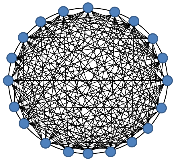
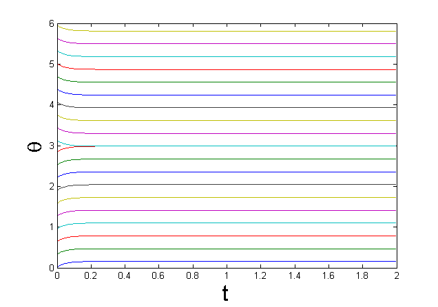
Figure 1: Twenty particles on unit circle with all-to-all sensing graph (left figure) and the simulation result(right figure) of (4) are demonstrated.

In the unit circle space, a sufficient condition for the permanent contraction of a convex hull is stated in the following theorem.

Theorem II.3 ([5, 13])

Consider the coupled oscillator model (3) with a connected graph $\mathcal{G}(\mathcal{V},\mathcal{E},\mathcal{A})$. Suppose that a convex hull of all initial values is within an open semi circle. Then, this convex hull is positively invariant, and each trajectory originating in the convex hull achieves an exponential synchronization.

The fundamental difference between a consensus protocol (1) in Euclidean space and another protocol (3) in unit circle space is the non-convex nature of configuration spaces like circle or sphere. For this reason, a global convergence analysis of the consensus algorithm in nonlinear space is quite intractable and at least very dependent on the communication graph[12].

In this paper, instead of controlling the orientation to be aligned, we estimate the orientation by using auxiliary variables defined on the higher dimensional vector spaces rather than unit circle space. Although consensus algorithm plays still important role in the proposed method, unlike the alignment law (3), the proposed method achieves global convergence of the estimated variables. This is described in the next section.

II-C Problem Statement

Consider $N$ single-integrator modeled mobile agents in the space: $\dot{p}_{i}=u_{i}~{},~{}i=1,\dots N,$ where ${p}_{i}\in\mathbb{R}^{3}$ and $u_{i}\in\mathbb{R}^{3}$ denote the position and control input, respectively, of agent $i$ with respect to the global reference frame, which is denoted by ${}^{g}\sum$. Following the notions of [15], we assume that agent $i$ maintains its own local reference frame with the origin at $p_{i}$. An orientation of $i$-th local reference frame with respect to the global reference frame is identified by a proper orthogonal matrix $C_{i}\in\mathrm{SO}(3)$ as illustrated in Fig. 2. By adopting a notation in which superscripts are used to denote reference frames, the dynamics of agents are described as $\dot{{p}}_{i}^{i}=u_{i}^{i},~{}i=1,\dots N,$ where ${{p}}_{i}^{i}\in\mathbb{R}^{3}$ and $u_{i}^{i}\in\mathbb{R}^{3}$ denote the position and control input, respectively, of agent $i$ with respect to ${}^{i}\sum$. For a weighted directed graph $\mathcal{G}=(\mathcal{V},\mathcal{E},\mathcal{A})$, agent $i$ measures the relative positions of its neighboring agents with respect to ${}^{i}\sum$ as:

$$p^{i}_{ji}:=p_{j}^{i}-p_{i}^{i},~{}j\in\mathcal{N}_{i},i\in\mathcal{V}.$$ (5)

We note that $p_{j}-p_{i}=C_{i}^{-1}(p_{j}^{i}-p_{i}^{i})$, because the local reference frames are oriented as much as the rotation matrix $C_{i}$ from the global reference frame.

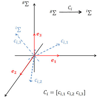
Figure 2: The local coordinate frame of $i$-th agent is rotated from the global reference frame $\left({}^{g}\sum\right)$ by $C_{i}$. $\{e_{i,1},e_{i,2},e_{i,3}\}$ is the set of orthonormal bases of $i$-th local frame ${}^{i}\sum$.

In this paper, we attempt to estimate $C_{i}$ by using the relative orientation measurement. Then, the estimated orientation is used to calibrate $C_{i}$ for the formation control. Let the desired formation $\mathbb{p}^{*}=(p_{1}^{*},\dots,p_{N}^{*})\in\mathbb{R}^{3N}$ be given. The formation problem is then stated as follows:

Problem II.1

Consider $N$-agents modeled by (1). Suppose $\mathcal{G}=(\mathcal{V},\mathcal{E},\mathcal{A})$ is the interaction graph of the agents. For a common reference frame ${}^{a}\sum$, design a control law such that $p_{j}^{a}-p_{i}^{a}\rightarrow p_{j}^{*}-p_{i}^{*}$ as $t\rightarrow\infty$ for all $i,j\in\mathcal{V}$ based on the measurements such as the relative displacement and relative orientation, which are measured in local coordinate frames of each agent.

We next formulate the localization problem. Under the same assumption of the Problem II.1, we desire to estimate the position of each agent. We denote $\hat{p}_{i}$ as the estimated position of $p_{i}$ with respect to the global reference frame. Then, the localization problem is stated in follows:

Problem II.2

Consider $N$-agents modeled by (1). Suppose $\mathcal{G}=(\mathcal{V},\mathcal{E},\mathcal{A})$ is the interaction graph of the agents. For each agent $i\in\mathcal{V}$, design an estimation law of $\hat{p}_{i}$ such that $\|\hat{p}_{j}-\hat{p}_{i}\|\rightarrow\|p_{j}-p_{i}\|$ as $t\rightarrow\infty$ for all $j\in\mathcal{V}$ based on the measurements such as the relative displacement and relative orientation, which are measured in local coordinate frames of each agent.

The following section proposes a method for the orientation estimation by using only relative orientation measurement. We describe the estimation method in general $n$-dimensional space instead of 3-dimensional space.

III Novel Method for Orientation Estimation

Orientation or attitude is often represented using three or four parameters in 3-dimensional space. Three or four-parameter representations include the unit-quaternions, axis-angle and Euler angles. While these parameters cannot represent orientation globally nor uniquely, the rotation matrix in $\mathrm{SO}(n)$ is unique and globally defined[16].

The orientation in the $n$-dimensional space is defined by an $n\times n$ proper orthogonal matrix $C\in\mathrm{SO}(n)$ containing, as column vectors, the unit vectors $\mathbb{c}_{i}(i=1,2,\dots n)$ identifying the orientation of the local frame with respect to the reference frame. A matrix $C$ has properties such as $C^{T}C=I$ and $\mathrm{det}(C)=+1$. When the common reference frame is the Cartesian coordinate system with standard basis $\mathbb{e}_{i}$$(i=1,\dots,n)$, the orientation of local frame is represented as $\mathbb{c}_{i}=C\mathbb{e}_{i}$ which is the $i$-column vector of $C$.

III-A Orientation estimation in $\mathrm{SO}(n)$

Consider $N$ agents whose interaction graph is $\mathcal{G}$ that has a spanning tree in $n$-dimensional space. Each agent does not share a common reference frame. It follows that the $i$-th local reference frame is rotated from the global reference frame with the amount of $C_{i}\in\mathrm{SO}(n)$. Let us suppose that $C_{ji}$ denotes the orientation of $j$-th local reference frame with respect to the $i$-th local reference frame. It provides $i$-th agent view to the $j$-th local reference frame with respect to the $i$-th local reference frame. If the global reference frame has the standard basis, each basis of $i$-th local frame with respect to the global reference frame is the column vector of $C_{i}$. It is well-known that $C_{ji}$ is defined by the multiplication of two rotation matrices as follows:

$$C_{ji}=C_{j}C_{i}^{-1}=C_{j}C_{i}^{T}$$ (6)

We assume that the $i$-th agent measures the orientation of $j$-th agent with respect to the $i$-th local reference frame. Therefore, $C_{ji}$ is obtained by the measurement. Let $\hat{C}_{i}\in\mathrm{SO}(n),\forall i\in\mathcal{V}$ be an estimated orientation which is the proper orthogonal matrix. Orientation estimation problem can be stated as follows:

Problem III.1

Consider $N$-agents whose interaction graph is $\mathcal{G}$ in $n$-dimensional space. For the common orientation which is identified by $C^{*}\in\mathrm{SO}(n)$, design an estimation law such that $C_{i}(t)^{T}\hat{C}_{i}\rightarrow C^{*}$ as $t\rightarrow\infty$ for all $i\in\mathcal{V}$ based on the relative orientation (6).

Let us denote $B_{i}\in\mathrm{SO}(n)$ which is defined as

$$B_{i}:=C_{i}X~{},~{}X\in\mathrm{SO}(n),\forall i\in\mathcal{V}.$$ (7)

According to (6), it follows that

$$B_{j}=C_{ji}B_{i}~{},~{}\forall(i,j)\in\mathcal{E}.$$ (8)

Under the assumption of Problem III.1, finding the steady state solution of $\hat{C}_{i}$ is equivalent to finding $B_{i}$ satisfying the equality (8). Then, Problem III.1 can be restated as follows:

Problem III.2

Under the assumption of Problem III.1, design an evolutionary algorithm for $B_{i}:[0,\infty)\rightarrow\mathbb{R}^{n\times n}$ such that

• $B_{i}(t)\in\mathrm{SO}(n)~{},~{}\forall t\in[0,\infty)$

• $B_{j}(t)\rightarrow C_{ji}B_{i}(t)$ as $t\rightarrow\infty$ , $\forall(i,j)\in\mathcal{E}$

Let us suppose that $n-1$ auxiliary variables are generated at each agent. Each auxiliary variable at $i$-th agent is denoted by $z_{i,k}\in\mathbb{R}^{n},k\in\{1,2,\dots,n-1\}$. Let $B_{i}$ be represented as $B_{i}=[b_{i,1},b_{i,2},\dots,b_{i,n}]$ where $b_{i,k}\in\mathbb{R}^{n},k\in\{1,\dots n\}$, is a $k$-th column vector of $B_{i}$. To generate orthonormal column vectors of $B_{i}$ from $z_{i,k}$ , we can use Gram-Schmidt process with any independent vectors $z_{i,k}\forall k\in\{1,\dots n-1\}$ as follows:

$$\begin{array}[]{ll}v_{i,1}:=z_{i,1}&,b_{i,1}:=\frac{v_{i,1}}{\|v_{i,1}\|}\\ v_{i,2}:=z_{i,2}-\langle z_{i,2},b_{i,1}\rangle b_{i,1}&,b_{i,2}:=\frac{v_{i,2}}{\|v_{i,2}\|}\\ \quad\vdots&~{}~{}~{}~{}~{}~{}~{}\vdots\\ v_{i,m}:=z_{i,m}-\sum_{k=1}^{m-1}\langle z_{i,m},b_{i,k}\rangle b_{i,k}&,b_{i,m}:=\frac{v_{i,m}}{\|v_{i,m}\|}\end{array}$$ (13)

where $m=n-1$ and $\langle\cdot,\cdot\rangle$ denotes the operator of inner product. The rest of the procedure include determining $b_{i,n}$ such that the determinant of $B_{i}$ is equivalent to $1$. We consider $b_{i,n}$ as a pseudovector for making det($B_{i}$) to be one. Pseudovector is a quantity that transforms like a vector under a proper rotation. In $n$-dimensional vector space, a pseudovector can be derived from the element of the ($n-1$)-th exterior powers, denoted $\wedge^{(n-1)}(\mathbb{R}^{n})$. It follows that

$$b_{i,1}\wedge b_{i,2}\wedge\cdots\wedge b_{i,n-1}.$$ (14)

Since every vector can be written as a linear combination of basis vectors, $\wedge^{(n-1)}(\mathbb{R}^{n})$ can be expanded to a linear combination of exterior products of those basis vectors. The pseudovector can be obtained from coefficients of (14). Since we obtain $b_{i,n}$ from the formalization of pseudovector, the matrix $B_{i}$ is a proper rotation.

This is one way to calculate the quantity $b_{i,n}$ in higher dimensional space, while there is no natural identification of $\wedge^{(n-1)}(\mathbb{R}^{n})$ with $\mathbb{R}^{n}$. Another convention for obtaining $b_{i,n}$ with proper rotation $B_{i}$ is stated in [8].

Now, we consider a second goal of the Problem III.2. We propose a single integrator model for dynamics of auxiliary variables as follows :

$$\dot{z}_{i,k}=u_{i,k}\quad,\forall i\in\mathcal{V},\forall k\in\{1,\dots,n-1\}.$$ (15)

Under the assumption of the Problem III.1, a control law for (15) is designed as follows for all $i\in\mathcal{V}$ and $k\in\{1,\dots,n-1\}$:

$$u_{i,k}=\sum_{j\in\mathcal{N}_{i}}a_{ij}(C_{ji}^{-1}z_{j,k}-z_{i,k})$$ (16)

where $a_{ij}>0$. From the definition of $C_{ji}$, we have $C_{ji}^{-1}=C_{ji}^{T}=C_{ij}$. Let $\mathbb{z}_{k}$ be a stacked vector form defined by $\mathbb{z}_{k}:=(z_{1,k},z_{2,k},\dots,z_{N,k})$. Here, (15)-(16) can be written in terms of $\mathbb{z}_{k}$ as follows:

$$\dot{\mathbb{z}}_{k}=H\mathbb{z}_{k}$$ (17)

where $H\in\mathbb{R}^{nN\times nN}$ is a block matrix which is defined as

$$H:=\left[\begin{array}[]{cccc}H_{11}&H_{12}&\cdots&H_{1N}\\ H_{21}&H_{22}&\cdots&H_{2N}\\ \vdots&\vdots&\ddots&\vdots\\ H_{N1}&H_{N2}&\cdots&H_{NN}\\ \end{array}\right]$$ (22)

Each partition $H_{ij}\in\mathbb{R}^{n\times n}$ is written as follows:

$$H_{ij}=\left\{\begin{array}[]{cl}a_{ij}C_{ij}&,j\in\mathcal{N}_{i}\\ -\sum_{j\in\mathcal{N}_{i}}a_{ij}I_{n}&,i=j\\ \mathbb{0}_{n}&,j\notin\mathcal{N}_{i}\end{array}\right.$$ (26)

where $\mathbb{0}_{n}\in\mathbb{R}^{n\times n}$ is a matrix having only zero entries.

III-B Analysis of the Stability

Let us consider the eigenvalue of $H$. By using a nonsingular matrix $D$, similarity transformation can be achieved as follows : $\bar{H}:=D^{-1}HD$. Suppose that $D$ is a block diagonal matrix defined by $D:=\operatornamewithlimits{diag}(C_{1},C_{2},\dots,C_{N})$ where $C_{i}\in\mathbb{R}^{n\times n}$, $i=\{1,\dots N\}$. Suppose that $\bar{H}_{ij}\in\mathbb{R}^{n\times n}$ denotes a partition of $i$-th row and $j$-th column in the block matrix $\bar{H}$. $\bar{H}_{ij}$ is written as follows :

$$\bar{H}_{ij}=C_{i}^{T}H_{ij}C_{j}=\left\{\begin{array}[]{cl}a_{ij}I_{n}&,j\in\mathcal{N}_{i}\\ -\sum_{j\in\mathcal{N}_{i}}a_{ij}I_{n}&,i=j\\ \mathbb{0}_{n}&,j\notin\mathcal{N}_{i}.\end{array}\right.$$ (30)

From (30), $\bar{H}$ is rewritten as $\bar{H}=-L_{H}\otimes I_{n}$ where $L_{H}\in\mathbb{R}^{N\times N}$ has zero row sum with dominant diagonal entries. From the Theorem II.1, all eigenvalues of $L_{H}$ have strictly positive real part except for a simple zero eigenvalue with corresponding eigenvector $\xi=(1,1,\dots,1)\in\mathbb{R}^{N}$.

Let us consider a coordinate transformation as $\mathbb{z}_{k}=D\mathbb{q}_{k}$. Then (17) is rewritten as follows:

$$\mathbb{\dot{q}}_{k}(t)=-L_{H}\otimes I_{n-1}{\mathbb{q}}_{k}(t),~{}~{}\forall k\in\{1,\dots,n-1\}$$ (31)

From the Theorem II.2, it is clear that $\mathbb{q}_{k}$ converges to the equilibrium set which is indicated as $\mathcal{E}_{q}=\{\mathbb{x}=(x_{1},x_{2},\dots,x_{N})\in\mathbb{R}^{nN}:x_{1}=x_{2}=\cdots=x_{N}\}$. For the estimation of orientation, we have to avoid the convergence of variables $\mathbb{q}_{k}$ to zero. Therefore, the desired equilibrium set is defined by $\mathcal{S}_{q}:=\mathcal{E}_{q}\setminus\{0\}$. For a square matrix $A$, define the column space of matrix $A$ as $\mathbb{C}(A)$. Then, we have the relationship $\mathbb{C}(A)=\rm{null}$$(A^{T})^{\perp}$, where $\mathrm{null}$$(A^{T})^{\perp}$ denotes the orthogonal space of null space of $A^{T}$. Based on the consensus property mentioned in the previous section, the following lemma provides conditions for the convergence of $\mathbb{q}_{k}$ to $\mathcal{S}_{q}$.

Lemma III.1

Suppose that $\mathcal{G}$ has a rooted-out branch. For the dynamics (31), there exists a finite point $\mathbb{q}^{\infty}_{k}\in\mathcal{S}_{q}$ for each $k\in\{1,\dots n-1\}$ such that $\mathbb{q}_{k}$ exponentially converges if and only if an initial value $\mathbb{q}_{k}(t_{0}),\forall k\in\{1,2,\dots,n-1\}$ is not in $\mathbb{C}(L_{H}\otimes I_{n})$.

Proof:

From the Theorem II.2, $\mathbb{q}_{k},\forall k\in\{1,2,\dots n-1\}$ globally exponentially converges to $\mathcal{E}_{q}$. Then, for each $k\in\{1,2,\dots n-1\}$, there exists a finite point $\mathbb{q}^{\infty}_{k}\in\mathcal{E}_{q}$ and constants $\lambda_{q},\eta_{q}>0$ such that

$$\|\mathbb{q}_{k}(t)-\mathbb{q}^{\infty}_{k}\|\leq\eta_{q}\mathrm{e}^{-\lambda_{q}(t-t_{0})}\|\mathbb{q}_{k}(t_{0})-\mathbb{q}^{\infty}_{k}\|.$$ (32)

Now, we consider a steady state solution $\mathbb{q}^{\infty}_{k}$. A solution of $\mathbb{q}_{k}$ is written as follows:

$$\mathbb{q}_{k}(t)=\mathrm{e}^{-L_{H}\otimes I_{n}(t-t_{0})}\mathbb{q}(t_{0}).$$ (33)

The Jordan form of $L_{H}$ is obtained by the similarity transformation as follows: $G^{-1}L_{H}G=J$. Let $G$ and $G^{-1}$ be represented as $G=[g_{1}~{}\cdots~{}g_{N}]$ and $G^{-1}=[w_{1}^{T}~{}\cdots~{}w_{N}^{T}]^{T}$ respectively. We supposed that $g_{N}$ is the right eigenvector of the zero eigenvalue. Then, $w_{N}$ is the left eigenvector of the zero eigenvalue. Since every nonzero eigenvalue of $L_{H}$ has negative real part, the state transition matrix $e^{J\otimes I_{n}(t-t_{0})}$ has the following form as $t\rightarrow\infty$.

$$\mathrm{e}^{J\otimes I_{n}(t-t_{0})}\rightarrow\left[\begin{array}[]{cccc}0&&&\\ &0&&\\ &&\ddots&\\ &&&1\end{array}\right]\otimes I_{n}$$ (38)

From (38), the steady state solution of $\mathbb{{q}}_{k}$ is as follows:

$$\lim_{t\rightarrow\infty}\mathbb{q}_{k}(t)$$

$$\quad=\lim_{t\rightarrow\infty}(G\otimes I_{n})\mathrm{e}^{J\otimes I_{n}(t-t_{0})}(G^{-1}\otimes I_{n})\mathbb{q}_{k}(t_{0})$$

$$\quad=(g_{N}\otimes I_{n})(w_{N}\otimes I_{n})\mathbb{q}_{k}(t_{0})$$

$$\quad=(g_{N}w_{N}\otimes I_{n})\mathbb{q}_{k}(t_{0})$$ (39)

This implies that $\mathbb{q}_{k}(t)$ converges to zero if and only if $\mathbb{q}_{k}(t_{0})$ is perpendicular to the $w_{N}\otimes I_{n}$ which is the left eigenvector of the zero eigenvalue. Then, it follows that $(w_{N}\otimes I_{n})\mathbb{q}_{k}(t_{0})=0$ if and only if $\mathbb{q}_{k}(t_{0})$ is in $\rm{null}$$(L_{H}^{T}\otimes I_{n})^{\perp}$. Since $\rm{null}$$(L_{H}^{T}\otimes I_{n})^{\perp}=\mathbb{C}(L_{H}\otimes I_{n})$, it completes the proof. ∎

The result of Lemma III.1 implies $\lim_{t\rightarrow\infty}\mathbb{z}_{k}(t)=D\mathbb{q}_{k}^{\infty}$ for each $k$. Let $B_{i}\in\mathrm{SO}(n)$ be derived from the procedure including Gram-Schmidt process of $z_{i,k},\forall k\in\{1,\dots n-1\}$ and the calculation of $b_{i,n}$. Consequently, there exists $P^{\infty}_{i}\in\mathrm{SO}(n)$ to which $B_{i}$ converges. We can show that $B_{i}(t)\rightarrow C_{ij}B_{j}(t),(i,j)\in\mathcal{E}$ as $t\rightarrow\infty$ from the following result.

Theorem III.1

Let $C_{i}\in\mathrm{SO}(n)$ denote a rotation matrix which identifies the orientation of the $i$-th agent. Suppose that $n\times n$ matrix $B_{i}$ for the $i$-th agent is derived from the procedures (13), (14) and (17). Then, there exists a common matrix $X\in\mathrm{SO}(n)$ such that $B_{i}$ converges to $C_{i}X$ as $t\rightarrow\infty$ for all $i\in\{1,\dots N\}$.

Proof:

By using the coordinate transformation, we define $q_{i,k}\in\mathbb{R}^{n}$ for all $i\in\{1,\dots N\}$ and $k\in\{1,\dots,n-1\}$ such that $z_{i,k}=C_{i}q_{i,k}$. Let us replace the value of $q_{i,k}$ with $z_{i,k}$ in the procedure (13). From the definition of $b_{i,k}$ for all $k$ in (13), $v_{i,k}$ is rewritten as follows :

$$\begin{array}[]{rl}v_{i,1}&=C_{i}q_{i,1}:=C_{i}x_{i,1}\\ v_{i,2}&=C_{i}q_{i,2}-\langle C_{i}q_{i,2},\frac{v_{i,1}}{\|v_{i,1}\|}\rangle\frac{v_{i,1}}{\|v_{i,1}\|}\\ &:=C_{i}x_{i,2}\\ \ \quad\vdots\\ v_{i,n-1}&=C_{i}q_{i,n-1}-\sum_{k=1}^{n-2}\langle C_{i}q_{i,n-1},\frac{v_{i,k}}{\|v_{i,k}\|}\rangle\frac{v_{i,k}}{\|v_{i,k}\|}\\ &:=C_{i}x_{i,n-1}\end{array}$$ (46)

Using this to replace $v_{i,m}$ by $x_{i,m},\forall m\in\{1,\dots n\}$, $x_{i,m}$ can be written as follows:

$$\begin{array}[]{rl}x_{i,1}&=q_{i,1}\\ x_{i,2}&=q_{i,2}-\langle q_{i,2},\frac{x_{i,1}}{\|x_{i,1}\|}\rangle\frac{x_{i,1}}{\|x_{i,1}\|}\\ \quad\vdots\\ x_{i,n-1}&=q_{i,n-1}-\sum_{k=1}^{n-2}\langle q_{i,n-1},\frac{x_{i,k}}{\|x_{i,k}\|}\rangle\frac{x_{i,k}}{\|x_{i,k}\|}\end{array}$$ (51)

This is a Gram-Schmidt procedure with respect to the $q_{i,k},\forall k\in\{1,\dots n-1\}$. From the result of Lemma III.1, for each $k$, $q_{i,k}$ converges to a finite point $q_{k}^{\infty}\in\mathbb{R}^{n}$ as $t\rightarrow\infty$ for all $i\in\mathcal{V}$. This implies that there exists a finite vector $x_{k}^{\infty}\in\mathbb{R}^{n}$ such that $\{x_{i,1},x_{i,2}\cdots x_{i,n-1}\}\rightarrow\{x_{1}^{\infty},x_{2}^{\infty},\cdots x_{n-1}^{\infty}\}$ as $t\rightarrow\infty$ for all $i$. It is clear that $b_{i,k}$ and $x_{i,k}$ have the following relationship: $b_{i,k}=C_{i}\frac{x_{i,k}}{\|x_{i,k}\|},\forall k\in\{1,2\dots n-1\}$. We also derive $b_{i,n}$ from (14). Therefore, in the steady state of $x_{i,k}$, we have the following solution of $B_{i}(t)$:

$$\lim_{t\rightarrow\infty}B_{i}(t)=C_{i}\left[\frac{x_{1}^{\infty}}{\|x_{1}^{\infty}\|}\frac{x_{2}^{\infty}}{\|x_{2}^{\infty}\|}\cdots\frac{x_{n}^{\infty}}{\|x_{n}^{\infty}\|}\right],\quad\forall i\in\mathcal{V}$$ (52)

It completes the proof. ∎

Since $B_{i}(t)\rightarrow C_{i}X$ as $t\rightarrow\infty$, it is clear that $B_{i}(t)\rightarrow C_{ij}B_{j}(t)$ as $t\rightarrow\infty$. From the result of Theorem III.1, we now see that the proposed algorithm provides the solution of the Problem III.2. Since we transformed the Problem III.1 to Problem III.2, $B_{i}$ is the estimated orientation.

In the following section, we combine this algorithm with the formation control. For a practical reason, we consider the formation control in 3-dimensional spaces instead of the general $n$-dimensional spaces.

IV Formation Control In 3-D Space

In 3-dimensional space, we have to obtain the matrix $B_{i}\in\mathrm{SO}(3)$ satisfying conditions stated in Problem III.2. We have two auxiliary variables denoted by $z_{i,1},z_{i,2}$ for the $i$-th agent. By using the proposed estimation law (17) and Gram-schmidt process, we can obtain $b_{i,1}$ and $b_{i,2}$. Since the pseudovector is directly calculated by using a cross product of two vectors in 3-dimensional space, the quantity $b_{i,3}$ is as follows :

$$b_{i,3}=b_{i,1}\times b_{i,2},~{}~{}~{}\forall i\in\mathcal{V}.$$ (53)

Note that $\hat{C}_{i}(t)=B_{i}(t)\in\mathrm{SO}(3)$. We now propose a control law for the formation system under the assumption of Problem II.1. Consider the following control law:

$$u_{i}^{i}=k_{u}\sum_{j\in\mathcal{N}_{i}}l_{ij}((p^{i}_{j}-p_{i}^{i})-\hat{C}_{i}(p_{j}^{*}-p_{i}^{*}))$$ (54)

where $k_{u}>0$ and $l_{ij}>0$. Since $u_{i}=C_{i}^{-1}u_{i}^{i}$, the position dynamics of $i$-th agent with respect to the global reference frame is written as follows:

$$\dot{p}_{i} = u_{i}=C_{i}^{-1}u_{i}^{i}$$ (55)

$$= k_{u}\sum_{j\in\mathcal{N}_{i}}l_{ij}C_{i}^{-1}\left((p^{i}_{j}-p_{i}^{i})-\hat{C}_{i}(p_{j}^{*}-p_{i}^{*})\right)$$ (56)

$$= k_{u}\sum_{j\in\mathcal{N}_{i}}l_{ij}\left((p_{j}-p_{i})-C_{i}^{-1}\hat{C}_{i}(p_{j}^{*}-p_{i}^{*})\right)$$ (57)

From the Theorem III.1, there exists $C^{*}\in\mathbb{R}^{3\times 3}$ such that $C_{i}^{-1}\hat{C}_{i}(t)$ converges to $C^{*}$ as $t\rightarrow\infty$. By defining ${e}_{i}:=p_{i}-C^{*}p_{i}^{*}$, we obtain the error dynamics as follows:

$$\dot{{e}}_{i} = k_{u}\sum_{j\in\mathcal{N}_{i}}l_{ij}({e}_{j}-{e}_{i})$$ (58)

$$+\underbrace{k_{u}\sum_{j\in\mathcal{N}_{i}}l_{ij}(C^{*}-C^{-1}_{i}\hat{C}_{i})(p_{j}^{*}-p_{i}^{*})}_{w_{i}:=}$$

Then, (58) can be rewritten in the vector form as follows:

$$\mathbb{\dot{e}}=-k_{u}L\otimes I_{3}\mathbb{e}+\mathbb{w}$$ (59)

where $\mathbb{e}=({e}_{1},\dots,{e}_{N})$ and $\mathbb{w}=(w_{1},\dots,w_{N})$. From (33) and the result of the Theorem III.1, it is clear that $C_{i}^{-1}\hat{C}_{i}$ converges to $C^{*}$ with an exponential rate. It follows that there exist $k_{w}>0$ and $\lambda_{w}>0$ such that

$$\|\mathbb{w}(t)\|\leq k_{w}\mathrm{e}^{-\lambda_{w}(t-t_{0})}\|\mathbb{w}(t_{0})\|$$ (60)

Now, we consider the solution of $\mathbb{e}(t)$ given by

$$\mathbb{e}(t)=\mathrm{e}^{-L\otimes I_{3}(t-t_{0})}\mathbb{e}(t_{0})+\int^{t}_{t_{0}}\mathrm{e}^{-L\otimes I_{3}(t-\tau)}\mathbb{w}(\tau)d\tau.$$ (61)

By using the result in Theorem 3.1 of [5], the following result is obtained.

Theorem IV.1

Under the estimation law (17) and the formation control law (54), there exists a finite point $p_{\infty}$ such that $p_{i}(t),\forall i\in\mathcal{V}$ globally exponentially converges to $C^{*}p_{i}^{*}+p_{\infty}$, if $\mathcal{G}$ has a rooted-out branch, and $\mathbb{\hat{q}}_{k}(t_{0}),\forall k\in\{1,2\}$is not in $\rm{C}$$(L_{H}\otimes I_{3})$.

Proof:

Let us define $\mathcal{E}_{e}$ as

$$\mathcal{E}_{e}:=\{(x_{1},\dots,x_{N})\in\mathbb{R}^{3N}:x_{i}=x_{j},\forall i,j\in\mathcal{V}\}$$ (62)

There exists $\mathbb{e}^{*}\in\mathcal{E}_{e}$, $k_{l}>0$ and $\lambda_{l}>0$ such that

$$\|\mathbb{e}(t)-\mathbb{e}^{*}\| \leq \left\|\mathrm{e}^{-L\otimes I_{3}(t-t_{0})}\mathbb{e}(t_{0})-\mathbb{e}^{*}\right\|$$ (64)

$$+\left\|\int^{t}_{t_{0}}\mathrm{e}^{-L\otimes I_{3}(t-\tau)}\mathbb{w}(\tau)d\tau\right\|$$

$$\leq k_{l}\mathrm{e}^{-\lambda_{l}(t-t_{0})}\|\mathbb{e}(t_{0})-\mathbb{e}^{*}\|$$ (66)

$$+\int^{t}_{t_{0}}\left\|\mathrm{e}^{-L\otimes I_{3}(t-\tau)}\right\|\left\|\mathbb{w}(\tau)\right\|d\tau$$

According to the definition of induced norm, $\left\|\mathrm{e}^{-L\otimes I_{3}(t-\tau)}\right\|$ is written as

$$\left\|\mathrm{e}^{-L\otimes I_{3}(t-\tau)}\right\|=\max_{\|\mathbb{x}\|=1,t_{0}\leq\tau\leq t}\left\|\mathrm{e}^{-L\otimes I_{3}(t-\tau)}\mathbb{x}\right\|\leq\eta$$ (67)

where $\eta>0$ is a finite value which bounds the matrix norm. It follows from (60) and (67) that

$$\int^{t}_{t_{0}}\left\|\mathrm{e}^{-L\otimes I_{3}(t-\tau)}\right\|\left\|\mathbb{w}(\tau)\right\|d\tau~{}~{}~{}~{}~{}~{}~{}~{}~{}~{}~{}~{}~{}~{}~{}~{}~{}~{}~{}~{}$$ (68)

$$\leq\int^{t}_{t_{0}}\eta k_{w}\mathrm{e}^{-\lambda_{w}(\tau-t_{0})}\left\|\mathbb{w}(t_{0})\right\|d\tau~{}~{}~{}~{}~{}~{}~{}$$ (69)

$$=\frac{-\eta k_{w}}{\lambda_{w}}\left[\mathrm{e}^{-\lambda_{w}(\tau-t_{0})}\right]^{t}_{t_{0}}\left\|\mathbb{w}(t_{0})\right\|~{}~{}~{}~{}~{}~{}~{}$$ (70)

$$=\frac{-\eta k_{w}}{\lambda_{w}}\left\|\mathbb{w}(t_{0})\right\|(\mathrm{e}^{-\lambda_{w}(t-t_{0})}-1)~{}~{}~{}~{}~{}~{}$$ (71)

From (71), (66) can be written as follows:

$$\|\mathbb{e}(t)-\mathbb{e}^{*}\| \leq k_{l}\mathrm{e}^{-\lambda_{l}(t-t_{0})}\|\mathbb{e}(t_{0})-\mathbb{e}^{*}\|$$ (73)

$$-\frac{\eta k_{w}}{\lambda_{w}}\left\|\mathbb{w}(t_{0})\right\|(\mathrm{e}^{-\lambda_{w}(t-t_{0})}-1).$$

By replacing $t_{0}$ with $t_{0}^{\prime}=(t+t_{0})/2$ in (73), we obtain

$$\|\mathbb{e}(t)-\mathbb{e}^{*}\| \leq k_{l}\mathrm{e}^{-\lambda_{l}\left(\frac{t-t_{0}}{2}\right)}\left\|\mathbb{e}(\frac{t+t_{0}}{2})-\mathbb{e}^{*}\right\|$$

$$-\frac{\eta k_{w}}{\lambda_{w}}\left\|\mathbb{w}(\frac{t+t_{0}}{2})\right\|(\mathrm{e}^{-\lambda_{w}\left(\frac{t-t_{0}}{2}\right)}-1)$$

$$\leq k_{l}^{2}\mathrm{e}^{-\lambda_{l}(t-t_{0})}\|\mathbb{e}(t_{0})-\mathbb{e}^{*}\|$$

$$-\frac{\eta k_{w}^{2}}{\lambda_{w}}\mathrm{e}^{-\lambda_{w}\left(\frac{t-t_{0}}{2}\right)}\left\|\mathbb{w}(t_{0})\right\|(\mathrm{e}^{-\lambda_{w}\frac{t-t_{0}}{2}}-1)$$

This completes the proof. ∎

V Network Localization in 3-D Space

Consider the agents under the assumption of Problem II.2. We can obtain $\hat{C}_{i}$ from the proposed estimation method for the unknown orientation as stated in the previous sections. Then, we design an estimation law of $\hat{p}_{i}$ as follows:

$$\dot{\hat{p}}_{i}=k_{u}\sum_{j\in\mathcal{N}_{i}}l_{ij}(\hat{p}_{j}-\hat{p}_{i}-\hat{C}_{i}^{T}p^{i}_{ji})$$ (74)

where $p_{ji}^{i}$ is a relative displacement defined in (5) and $k_{u},l_{ij}>0$. We know that $p^{i}_{ji}=p^{i}_{j}-p^{i}_{i}=C_{i}(p_{j}-p_{i})$. By defining $\tilde{p}_{i}$ as $\tilde{p}_{i}:=\hat{p}_{i}-C^{*}p_{i}$, we obtain the estimation error dynamics as follows :

$$\dot{\tilde{p}}_{i} = k_{u}\sum_{j\in\mathcal{N}_{i}}l_{ij}(\hat{p}_{j}-\hat{p}_{i}-\hat{C}_{i}^{T}C_{i}(p_{j}-p_{i}))$$ (75)

$$= k_{u}\sum_{j\in\mathcal{N}_{i}}l_{ij}\left(\tilde{p}_{j}-\tilde{p}_{i}\right)$$

$$+\underbrace{k_{u}\sum_{j\in\mathcal{N}_{i}}l_{ij}(C^{*}-\hat{C}_{i}^{T}C_{i})(p_{j}-p_{i})}_{\psi_{i}:=}$$

Thus the overall error dynamics for position estimation can be written as

$$\dot{\tilde{\mathbb{p}}}=-k_{u}L\otimes I_{3}\tilde{\mathbb{p}}+\Psi$$ (76)

where $\tilde{\mathbb{p}}=(\tilde{p}_{1},\tilde{p}_{2},\dots,\tilde{p}_{N})$ and $\Psi=(\psi_{1},\psi_{2},\dots\psi_{N})$. We notice that (76) corresponds to (59). We obtain the following corollary based on the relationship.

Corollary V.1

Under the orientation estimation law (17) and the position estimation law (74), there exists a finite point $\hat{p}^{\infty}_{i},\forall i\in\mathcal{V}$ to which $\hat{p}_{i}$ globally exponentially converges, such that $\|\hat{p}^{\infty}_{j}-\hat{p}^{\infty}_{i}\|=\|p_{j}-p_{i}\|$, if $\mathcal{G}$ has a rooted-out branch, and $\mathbb{\hat{q}}_{k}(t_{0}),\forall k\in\{1,2\}$is not in $\rm{C}$$(L_{H}\otimes I_{3})$.

VI Simulation Result

In this section, we provide simulation results to verify the proposed methods. We consider six agents whose interaction graph is illustrated in Fig. 3.

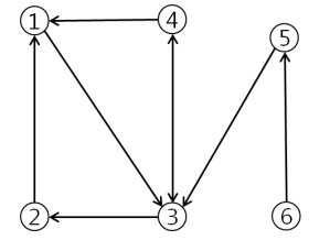
Figure 3: Interaction graph of six agents for simulation

Suppose that each agent has its own reference frame which is rotated from the global reference frame by the proper orthogonal matrix $C_{i}\in\mathbb{R}^{3\times 3},i=\{1,2,3,4,5,6\}$. For the simulation, the matrix $C_{i}$ is arbitrary determined. Estimated orientation of $i$-th agent identified by $\hat{C}_{i}$ can be obtained by using two auxiliary variables. Under the estimation law (17), $\hat{C}_{i}(t)$ converges to a steady state solution as $t$ goes to infinity. The formation control law (54) of $i$-th agent is simultaneously conducted with the estimation of orientation $\hat{C}_{i}$. According to the result of the Theorem IV.1, the position of $i$-th agent denoted by $p_{i}$ converges to $C^{*}p_{i}^{*}+p_{\infty}$, where $C^{*}\in\mathbb{R}^{3\times 3}$ is a common rotation matrix obtained by $C^{T}\hat{C}_{i}(t)$ as $t\rightarrow\infty$, $p_{i}^{*}$ is desired position of $i$-th agent, and $p_{\infty}$ is a common position vector. Fig. 4 shows the result that the measured displacement of neighboring agents converges to the desired displacement with rotational motion. Fig. 5 depicts that the formation of six agents using the proposed strategy, which includes a combination of orientation estimation and formation control law, converges to the rotated desired shape.

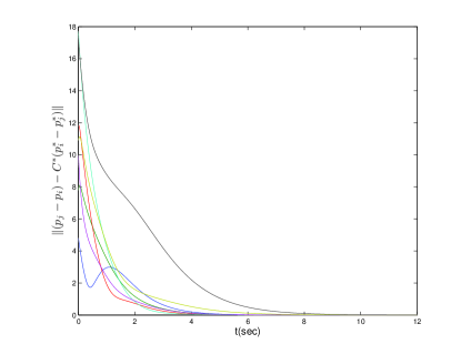
Figure 4: Difference of the measured displacement and the desired displacement of neighboring agents. $C^{*}$ is a common rotation matrix.

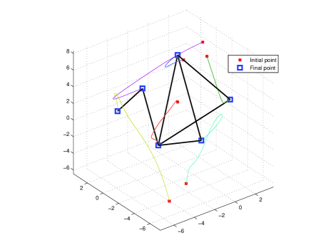
Figure 5: Formation control via orientation estimation in 3 dimensional space

VII Conclusion

In this paper, we proposed a novel estimation method for unknown orientation of agent with respect to the common reference frame in general $n$-dimensional space. We added virtual auxiliary variables for each agent. These auxiliary variables are corresponding to column vectors of estimated orientation $\hat{C}_{i}\in\mathrm{SO}(n)$. An estimation law of auxiliary variables is based on the principle of consensus protocol. Since configuration space for the proposed method is $n$-dimensional vector space instead of nonlinear space like unit circle, global convergence of auxiliary variables is guaranteed. Consequently, each desired point to which auxiliary variables converge, under the proposed estimation law, is transformed to the estimated orientation. This estimated frame is used to compensate the rotated frame of each agent in the formation control system. Under the formation control law with proposed estimation method, we guarantee a global convergence of multi-agent system to the desired shape in 3-dimensional space, under the distance-based setup. The proposed strategy can also be applied to the localization problem in networked systems. The result remedies the weak point of previous works [5, 6] where the range of initial orientations is constrained to $0\leq\theta_{i}<\pi$.

References

• [1] K.-K. Oh, M.-C. Park, and H.-S. Ahn, “A survey of multi-agent formation control,” Automatica, vol. 53, pp. 424–440, 2015.
• [2] Z. Lin, B. Francis, and M. Maggiore, “Necessary and sufficient graphical conditions for formation control of unicycles,” IEEE Transactions on Automatic Control, vol. 50, pp. 121–127, 2005.
• [3] W. Ren and E. Atkins, “Distributed multi-vehicle coordinated control via local information exchange,” Int. Journal of Robust and Nonlinear Control, vol. 17, pp. 1002–1033, 2007.
• [4] D. V. Dimarogonas and K. J. Kyriakopoulos, “A connection between formation inachievability and velocity alignment in kinematic multi-agent systems,” Automatica, vol. 44, no. 10, pp. 2648–2654, 2008.
• [5] K.-K. Oh and H.-S. Ahn, “Formation control and network localization via orientation alignment,” IEEE Trans. on Automatic Control, vol. 59, no. 2, pp. 540–545, Feb. 2014.
• [6] E. Montijano, D. Zhou, M. Schwger, and C. Sagues, “Distributed formation control without a global reference frame,” in Proceedings of Americal Control Control(ACC),2014, 2014, pp. 3862–3867.
• [7] B.-H. Lee and H.-S. Ahn, “Distributed formation control via global orientation estimation,” Automatica, vol. 73, pp. 125–129, 2016.
• [8] ——, “Distributed estimation for the unknown orientation of the local reference frames in n-dimensional space,” in Proc. Control Automation Robotics and Vision(ICARCV), 2016 14th International Conference on, Nov. 2016.
• [9] L. Moreau, “Stability of continuous-time distributed consensus algorithms,” in Decision and Control 2004. CDC. 43rd IEEE Conference on, Dec. 2004, pp. 3998 – 4003.
• [10] L. Scardovi and R. Sepulchre, “Synchronization in networks of identical linear systems,” Automatica, vol. 45, pp. 2557–2562, 2009.
• [11] A. Jadbabaie, J. Lin, and A. S. Morse, “Coordination of groups of mobile autonomous agents using nearest neighbor rules,” IEEE Transactions on Automatic Control, vol. 48, no. 6, pp. 988–1001, 2013.
• [12] R. Sepulchre, “Consensus on nonlinear spaces,” Annual Reviews in Control, vol. 35, pp. 56–64, 2011.
• [13] F. D$\rm{\ddot{o}}$rfler and F. Bullo, “Synchronization in complex networks of phase oscillator:a survey,” Automatica, vol. 50, no. 6, pp. 1539–1564, 2014.
• [14] L. Moreau, “Stability of multiagent systems with time-dependent communication links,” IEEE Trans. on Automatic Control, vol. 50, no. 2, pp. 169–182, Feb. 2005.
• [15] K.-K. Oh and H.-S. Ahn, “Formation control of mobile agents based on distributed position estimation,” IEEE Trans. on Automatic Control, vol. 58, no. 3, pp. 737–742, Mar. 2013.
• [16] N. Chaturvedi, A. Sanyal, and N. McClamroch, “Rigid-body attitude control,” IEEE Control Systems, vol. 31, no. 3, pp. 30–51, 2011.