An easy and efficient approach
for testing identifiability of parameters
Abstract
The feasibility of uniquely estimating parameters of dynamical systems from observations is a widely discussed aspect of mathematical modelling. Several approaches have been published for analyzing identifiability. However, they are typically computationally demanding, difficult to perform and/or not applicable in many application settings.
Here, an intuitive approach is presented which enables quickly testing of parameter identifiability. Numerical optimization with a penalty in radial direction enforcing displacement of the parameters is used to check whether estimated parameters are unique, or whether the parameters can be altered without loss of agreement with the data indicating non-identifiability. This Identifiability-Test by Radial Penalization (ITRP) can be employed for every model where optimization-based fitting like least-squares or maximum likelihood is feasible and is therefore applicable for all typical deterministic models.
The approach is illustrated and tested using 11 ordinary differential equation (ODE) models. The presented approach can be implemented without great efforts in any modelling framework. It is available within the free Matlab-based modelling toolbox Data2Dynamics (Raue et al., 2015). Source code is available at https://github.com/Data2Dynamics.
I Introduction
An essential step of mathematical modelling is estimation of parameters. Although the methodology is not restricted to ordinary differential equation (ODE) models, the focus in this paper is on this class of models because they are frequently used to describe the dynamics of molecular compounds, e.g. involved in signalling pathways or gene regulation networks. In this setting, parameters represent abundances of cellular compounds or their interaction strengths, but can also comprise scaling- or variance parameters for the measurements. Defining dynamic models by translating molecular interaction maps based on biochemical rate laws can lead to large and over-parameterized models where the data does not provide enough information for uniquely estimating parameters. This issue has been termed non-identifiability and occurs in all settings, where the level of detail of the model does not fit to the amount of experimental data.
For small models non-identifiabilities can be detected by analytical approaches, e.g. based on power series expansions (Pohjanpalo, 1978; Walter and Lecourtier, 1982), calculation of transfer matrices (Bellman and Astroem, 1970), differential algebra (Bellu et al., 2007; Ljung and Glad, 1994; Maria Pia Saccomani, 2003), similarity transformations (Vajda, 1981), Lie-group theory (Merkt et al., 2015), or by treating parameters as constant dynamic states and applying concepts from observability or controllability analyses (Travis and Haddock, 1981). For more realistic settings, numerical methods have been published which are based on the rank of the Jacobian (Catchpole and Morgan, 1997; Karlsson et al., 2012) or Fisher-Information (Hidalgo and Ayesa, 2001; Viallefont et al., 1998). Nonparametric transformations have been used in (Hengl et al., 2007) to find non-identifiable parameter relationships based on multi-start optimization results. In addition, the profile-likelihood has been suggested to investigate identifiability for given experimental data (Raue et al., 2009, 2011). Since this approach is tailored to nonlinear systems as they frequently occur in systems biology and it provides statistically valid confidence intervals, this method might be the currently most frequently applied approach in this field. However, calculation of likelihood profiles for all parameters is time-consuming, especially for large systems and there are recent efforts for developing computationally more efficient methods (Raman et al., 2017). Despite the multitude of approaches, the ongoing discussion and research in this field still indicates lack of efficient and broadly applicable approaches.
In this manuscript, penalized optimization is employed for testing of structural identifiability by an additional model fitting step. The penalty enters like an additional data point which is used to pull in the parameter direction where the data provides least information. This approach enables a fast and reliable procedure for identifiability analysis and thereby resolves a major bottleneck of mathematical modelling. The applicability is demonstrated for two illustration- and nine application models.
II Methods
In the following sections, the mathematical notation is introduced. Since several definitions and terms of identifiability/non-identifiability exists, different terminologies are also briefly summarized.
II.1 Model setting
Although the presented method is applicable for any model where parameters are estimated by maximum-likelihood or any other optimization-based fitting method, the discussion is restricted to ODE models in the systems biology context in the following. In this setting, chemical reaction laws are frequently utilized to define rate equations describing the dynamics
| (1) |
of concentrations . Different stimulations or perturbations are represented in the model by inputs . The inital values are either known or defined as additional parameters, i.e. . The dynamic states are linked to measurements
| (2) |
via observation functions , which might comprise scalings and/or transformations like a log-transformation. In this formulation, represents additive Gaussian noise although the approach is not restricted to this type of noise and other distributions can be considered by defining the likelihood with the respective density function for the measurement errors. In an easy setup, the magnitude of the experimental errors is constant, i.e. . In general, an error model
| (3) |
e.g. , might depend on and could also contain parameters like absolute or relative noise levels. Therefore, in a general formulation the parameter vector contains all unknown constants determining the dynamics, the predicted observations and the noise levels.
Note that a notation has been chosen where index enumerates individual measurements and each data point has an individual observation function for a specific experimental design (Kreutz and Timmer, 2009) given by the time point, observed state(s) as well as possible assignments to inputs, offset- or scaling parameters and error model . This notation emphasize that measurements are often performed for different but sparse combinations of observables/measurement techniques, stimulation/perturbations and time points and is therefore commonly used in statistics, e.g. for multivariate models like linear models, mixed effects models or survival models.
II.2 Parameter estimation and objective function
Maximum likelihood estimation
| (4) |
has several beneficial statistical properties like asymptotic normality, consistency and efficiency (Cox and Hinkley, 1994). For known Gaussian errors , least-squares estimation
| (5) |
with the least-squares objective function
| (6) |
is a special case of maximum likelihood estimation since the estimate coincides with because . If prior knowledge about some parameters is available, this can be accounted for by using a penalized log-likelihood
| (7) |
which in the case of Gaussian priors also yields a sum of quadratic terms and can be treated like additional data points. In the following, is used as a general place-holder for the objective function which is without loss of generality assumed to be minimized
| (8) |
for parameter estimation, i.e. might coincide with , or . Independently of the chosen objective function and its signum, we term as likelihood in the following.
II.3 Parameter identifiability
A variety of terms and definitions for non-identifiability are available in literature. In general, non-identifiability refers to lack of information for uniquely specifying the parameters. In this subsection, two complementary points of view are summarized.
II.3.1 Mathematical point of view
A series of papers consider a setting with predefined observables but without specifying observation noise nor number and location of time points. A widely used mathematical definition of non-identifiability (Oana-Teodora Chis, 2011) in this setting is: A parameter , is structurally locally identifiable if for almost any , there exists a neighbourhood such that if
| (9) |
If this property holds not only within a neighbourhood but for the whole parameter space, the parameter is termed structurally globally identifiable.
This formulation considers analysis of identifiability of model parameters for a given set observation functions. It is independent on the number and accuracy of data points and therefore fits well to applications settings where (almost) continuous and noise-free observations are feasible. In this setting, identifiability refers to a unique mapping from the observed dynamics to parameters (Ljung, 1999). In agreement with this, (Bellman and Astroem, 1970) defined structural identifiability already in 1970 as a unique minimum of
| (10) |
In many application disciplines like cell biology, however, the number of data points is limited and the measurements exhibit a non-neglectable amount of noise. Then, parameter identifiability depends on availability of measurements, e.g. on the number of data points and on the exact combinations of measurement times, input and observation functions. Moreover, non-identifiabilities occurring in parameters of the observation functions or error models have to be considered. Therefore, the mathematical definition (9) or (10) does only partly capture the effects occurring in inverse problems and can be reasonably extended by a formulation considering individual data points.
II.3.2 Statistical point of view
In a statistical formulation, parameter identifiability can be defined as a unique minimum of the log-likelihood (Little et al., 2010), e.g. in the least-squares setting as a unique minimum of
| (11) |
where summation is performed over all data points, i.e. over all combinations of input, observation function and measurement time. Moreover, as discussed above, summation can comprise additional terms originating from priors or estimation of noise levels.
For this setup, the profile likelihood
| (12) |
has been suggested for assessing identifiability (Raue et al., 2009) of a parameter . In (12), all parameters are optimized except for different values for . A parameter with a flat profile likelihood indicates non-unique parameter estimates because changing can be entirely compensated by refitting the other parameters. Such flat directions in the parameter space indicate redundant parametrizations. Therefore, the existence of flat likelihood profiles has been used to define structural non-identifiability (Raue et al., 2009). This property depends on the set of given observations , but is independent on the magnitude of observation noise because scaling all ’s only scales the objective function but does not impact existence of entirely flat manifolds.
Since the profile likelihood is applicable for any model which allows optimization-based estimation, it has become a standard approach in systems biology for assessing identifiability111Most citations for in Web of Science when searching for “identifiability analysis systems biology”. Using a proper threshold, the profile likelihood also enables the calculation of confidence intervals (Kreutz et al., 2011). In some cases, it might occur that a unique minimum exists, but the profile likelihood does not exceed the confidence threshold in lower and/or upper direction. Then, the confidence interval has infinite size. This effect only occurs in the case of measurement noise and it vanishes in the limit . Since averaging over replicates decreases the standard deviation this limit is asymptotically obtained by increasing the number of measurement replicates. Because this effects only occurs due to practical limitations in generating a sufficient number of replicates, it has been used to define practical non-identifiability (Raue et al., 2009). Both cases are difficult to distinguish in applications since the likelihood might be locally flat but could still exceed a significance threshold as shown later in section IV.3. Since discrimination between both scenarios is only a terminological issue and not the focus of the article, we do not further discuss this aspect. We use structural non-identifiability as synonym for locally flat likelihood and focus on detection of this property in the following.
III Approach
In the following, the major focus is the statistical point of view, i.e. identifiability is investigated for an inverse setting with given experimental data. In section III.5, the approach is adapted to investigate identifiability in the mathematical, i.e. continuous and noise-free context.
III.1 Testing identifiability
Existence of redundant parametrizations, i.e. presence of flat directions of the likelihood for a given data set, is investigated by penalized optimization. After standard model fitting, i.e. after parameters are estimated according to (11), we suggest usage of a penalized objective function
| (13) |
with
| (14) |
in to pull the parameter vector away from the estimated parameters . The penalty term is quadratic and has its minimum at a circular manifold with radius centered around . Parameters minimizing are denoted by , i.e.
| (15) |
The penalization strength is chosen by default as . Thereby, it holds with and the magnitude of the increase
| (16) |
of the objective function by penalization is after fitting in the interval and therefore easy to interpret.
is the major characteristic used to define the Identifiability-Test by Radial Penalization (ITRP). In the case of structural non-identifiability, the parameters can be altered and thereby minimize the penalty without reducing agreement with the data. Then, the penalty vanishes without increasing the data-related part of the objective function. Therefore indicates structural non-identifiability. In contrast, indicates that the model is structurally identifiable since the parameter cannot be moved by an euclidean distance without loss of agreement with the data. The Identifiability-Test by Radial Penalization (ITRP) suggested in this manuscript consists of an additional fit based on () and evaluation whether there is an increase of the objective function (16).
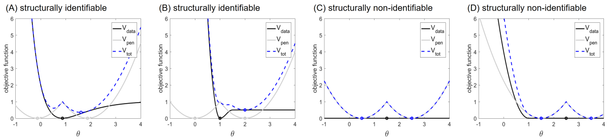
Because quadratic terms can be most efficiently optimized, the -norm has been used in (14) for calculating the distance between and as well as for penalizing the distance to the target radius . An alternative would be the -norm which could be used to enforce that the parameters are exactly at the sphere with radius . This however depends on and therefore requires a proper choice of . Moreover, optimization could be hampered due to non-continuous derivatives which would slow down the approach.
Fig. 1 shows possible scenarios for the trade-off between penalty and data agreement . Panel (B) corresponds to an identifiable setting with a unique minimum but a flat plateau which results in . This scenario shows that is better suited for assessing identifiability than evaluating whether is equal to .
III.2 Implementation
Fitting a model by numerical optimization requires integration of the ODEs and an implementation of the objective function as defined in (11). For efficient numerical optimization, this function should also calculate the derivatives . This is available in typical modelling toolboxes. In the following, we provide equations for implementing the ITRP introduced in the previous section.
For implementing the ITRP, the standard objective function used to fit a model has to be augmented via by adding the penalty term and by respectively adapting the derivative
| (17) |
with
| (18) |
The Hessian is given by
| (19) |
with
| (20) |
Some least-squares optimization routines like lsqnonlin (Coleman and Li, 1996; The MathWorks, ) use data residuals
| (21) |
and a Jacobian with
| (22) |
for optimization instead of a scalar objective function. These algorithms internally calculate the sum of squared residuals within the optimization routine and approximate the Hessian matrix by . For applying the identifiability test, the residual vector has to be augmented with the square-root of (14), i.e. by
| (23) |
and the derivatives with
| (24) |
Since the presented approach is numeric, a threshold is required to decide whether is larger than zero. A proper choice of depends on the accuracy of optimization e.g. on the termination thresholds. In our examples, we chose - which worked for all application examples. For properly choosing , we suggest to use a termination criterion for optimization which is based on minimal changes of the objective function , e.g. TolFun=1e-6 in Matlab notation (The MathWorks, ) instead of threshold based on parameter changes (TolX in Matlab notation).
In principle, a single penalized fit is sufficient to detect non-identifiability. However, to increase the robustness of the outcome with respect to non-converging fits we chose a multi-start strategy with five fits with different initial guesses throughout the manuscript. In the Supplementary Information we show the dependency on the number of fits and show that for all models two initial guesses, one using as starting point and one random choice, are sufficient to perform the ITRP.
III.3 Parameter subsets
In some applications, non-identifiability might only matter for a specific subset of the parameters, e.g. the dynamic parameters. Then, the exact values of other parameters, e.g. scaling parameters, might be of minor concern. In such a situation, only the parameters of interest should be used to define the penalty and (16) becomes
| (25) |
III.4 Iterative analysis
The parameter component
| (26) |
which the largest change due to penalized optimization can be termed as the least identifiable parameter. In the case of non-identifiability, this parameter index indicate a non-identifiable parameter, although the result might not be unique in the case of several non-identifiabilities. Fixing such a parameter enables investigation of the remaining non-identifiabilities. By repeatedly applying this procedure, the number of non-identifiabilities can be found, i.e. the number of parameters which have to be fixed (or estimated elsewhere) for obtaining an entirely identifiable model. This procedure is illustrated in the results section IV.3.
III.5 Investigating mathematical identifiability
Data-based non-identifiability (9) can be seen as a necessary but not sufficient prerequisite for mathematical non-identifiability which is based on continuous, noise-free observations. The ITRP introduced above can be adapted to also investigate mathematical identifiability. For this purpose, the limiting case has to be considered. This can be seen by comparing in (6) with the integral difference (10). The constant value used to replace measurement uncertainties is relevant for the ITRP from the numerical point of view for distinguishing increasing from non-increasing objective functions , i.e. has to be chosen properly in relation to the magnitude of the threshold .
We used the accuracy of numerical integration which is roughly specified by absolute and relative tolerances and of the numerical ODE intergration algorithm. In the Supplementary Information, mathematical identifiability is investigated for a pathway model with
| (27) |
where atol refers to the absolute integration tolerance and rtol to the relative. Since each time point where the dynamics is evaluated contributes to the objective function and the outcome should not dependent on the number of chosen data points used to evaluate the dynamics.
III.6 Scope and restrictions
The procedure is only applicable if the objective function used for parameter estimation is deterministic. This means, that the procedure does not reliably work for models with a stochastic dynamics. Moreover, the ITRP as presented above requires estimated parameters as starting point. Non-optimality of this parameters could be indicated by negative .
The presented approach rely on a reliably working optimization procedure. If optimization does not reliable work, flat directions are not found by penalized optimization. For the standard procedure using a single , this problem cannot be distinguished from an identifiable setting because in both cases the objective function increase due to penalization. In contrast, calculating the dependency of on on an interval might indicate an optimization problem by a non-smooth outcome (see IV.2). Another way to ensure that optimization works reliable enough, is to artifically introduce a non-identifiability, e.g. by replacing a parameter by a product of two parameters and then check as a positive-control whether such a non-identifiability is found.
Prespecified bounds for the parameters can be considered by restricting optimization to the feasible region. In fact, most of the application examples have parameter bounds which prevent failure of ODE integration. The definition of the feasible parameter space can be considered as part of the model structure.
IV Results
| Name | Identifiable? | Publication | ||
|---|---|---|---|---|
| ABC | 3 | 11∗ | Yes | Kreutz et al. (2011) |
| ABC_rel | 4 | 11∗ | No | |
| Bachmann | 113 | 542 | No | Bachmann et al. (2011) |
| Becker | 16 | 85 | Yes | Becker et al. (2010) |
| Boehm | 9 | 48 | Yes | Boehm et al. (2014) |
| Bruno | 16 | 46 | Yes | Bruno et al. (2016) |
| Raia | 39 | 205 | No | Raia et al. (2011) |
| Schwen | 30 | 292 | No | Schwen et al. (2015) |
| Swameye | 16 | 46 | No | Swameye et al. (2003) |
| Toensing-School | 5 | 15 | Yes | Tönsing et al. (2017) |
| Toensing-Zika | 17 | 57 | No | Tönsing et al. (2017) |
Two small illustration models as well as nine application models with real measurements were used to demonstrate the applicability and capabilities of the presented approach in this chapter. Table 1 provides an overview about the models which have between 3 and 113 estimated parameters and between 11 and 542 data points. Five models are structurally identifiable, six are structurally non-identifiable as shown in the Supplementary Information where the mostly cited approach (Raue et al., 2009) which is at the same also applicable for all investigated models has been applied as a reference.
IV.1 Illustration models
A small and illustrative model of two consecutive reactions
| (28) |
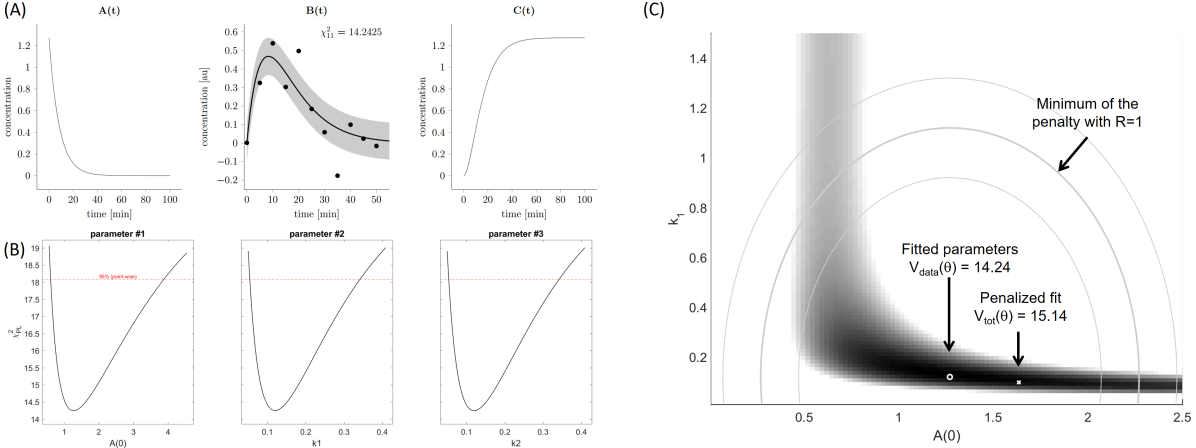
with rates and initial conditions is utilized to illustrate the ITRP. For the simulated measurements, normally distributed noise with has been assumed which corresponds to a typical signal-to-noise ratio for applications in molecular biology of around . For an identifiable setting, is assumed to be measured at . Although parameter log-transformation is reasonable for fitting ODE models (Kreutz, 2016), we omit the log-transformation for the illustration models in the figures to keep the setting as simple as possible. The identifiable model has a unique minimum and is termed ABC, see first row in Table 1.
For the simulated data shown in panel (A) in Fig. 2, the maximum likelihood estimate is . The profile likelihood for all parameters shown in panel (B) exhibit unique minima. Panel (C) shows , i.e. the dependency of the likelihood for given and while optimizing . The maximum likelihood estimate is indicated by the circle. If the penalty is added, the minimum shifts, but due to identifiability, the objective function increases: , i.e. which correctly indicates identifiability.
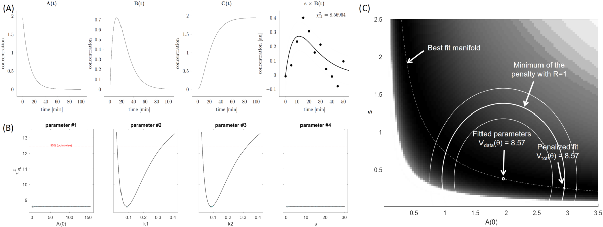
For a non-identifiable setting, it is assumed that is only measured on a relative scale, i.e. the observation function is
| (29) |
with scaling parameter . This model has four fitted parameters and is termed ABC_rel (2nd row in Table 1). Panel (A) in Fig. 3 shows the dynamics and the measurements . The profile likelihood of parameters and shown in panel (B) are flat indicating a non-unique minimum and non-identifiability. In the two-dimensional representation shown in panel (C), the parameters and are optimized for different combinations of and . The flat best-fit manifold is indicated by the dashed line.
If the ITRP is applied, the parameters are shifted due to the penalty but the objective function does not increase, i.e. which correctly indicates non-identifiability.
IV.2 Dependency on penalty location and parameter relationships
In (Raman et al., 2017), radial constraints have been used to define multi-scale sloppiness and combined with an integration-based approach to uncover non-identifiabilities and its corresponding parameter relationships. Such a procedure can be interpreted as calculation of a prediction profile likelihood
| (30) |
as suggested in (Kreutz et al., 2013) for predicting the radial, euclidean distance
| (31) |
to the estimated parameters.
In (Kreutz et al., 2013), is was shown that penalized optimization
| (32) |
can be used to calculate the solution of the constrained optimization in (30) in a numerically more robust manner for any kind of prediction . In our setting (31), penalties are exactly satisfied in the case of non-identifiability and therefore both profiles (30) and (32) coincide.
The ITRP, in turn, is equivalent to equation (32) for a single radius . For testing of non-identifiability, only one point at the profile (32) for the radial distance is sufficient. Here, the exact choice of specifies the definition of “local” according to the definition (9). Nevertheless, the function (32) can be used to obtain a more comprehensive picture and for assessing parameter relationship(s) as discussed in (Raue et al., 2009; Raman et al., 2017).
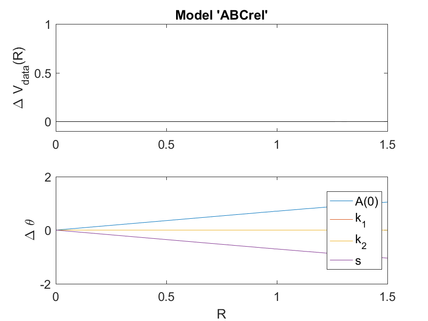
Fig. 4 shows the profile for the non-identifiable model ABC_rel. Flatness of the profile in the upper panel indicates non-uniqueness of the parameters, i.e. non-identifiability. The lower panel in Fig. 4 indicates that parameters and have to be adjusted for increasing penalties and are therefore in the flat, redundant manifold.
IV.3 Application models
| Name | Identifiability | Computation time |
|---|---|---|
| correct? | (rel. to profile likelihood) | |
| ABC | yes | 0.22 sec (0.96%) |
| ABC_rel | yes | 1.24 sec (2.47%) |
| Bachmann | yes | 9.05 sec (0.02%) |
| Becker | yes | 0.24 sec (0.25%) |
| Boehm | yes | 2.19 sec (2.48%) |
| Bruno | yes | 0.09 sec (0.38%) |
| Raia | yes | 4.50 sec (0.10%) |
| Schwen | yes | 8.40 sec (0.09%) |
| Swameye | yes | 0.66 sec (0.11%) |
| Toensing-School | yes | 0.12 sec (0.56%) |
| Toensing-Zika | yes | 0.80 sec (0.09%) |
As application examples, nine published models were analyzed as summarized in Table 1, rows 3-11. As in the original publication, the parameters were analyzed at the log10-scale. The outcome of the identifiability test is summarized in Table 2. As a reference, the profile likelihood approach (Raue et al., 2009) was used. Our new approach correctly assesses identifiability for all models and requires less than 1% computation times. The total computation time, i.e. the sum over all nine application models, was 26.1 seconds using five fits with five different initial guesses for each model but 1005.5 minutes for the profile likelihood approach, and 17.0 seconds vs. 252.7 minutes if the computationally most demanding model (Bachmann) is excluded. The command-line output of the implementation in Data2Dynamics modelling toolbox as well as the likelihood profiles are provided in detail in the Supplementary Information.
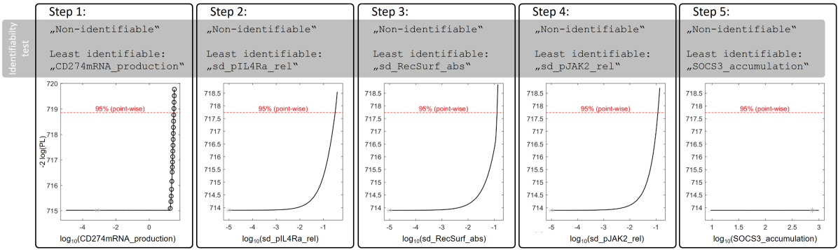
As representative example, the model published in (Raia et al., 2011) is shown in Fig. 5. For the published model, the identifiability test indicates non-identifiability and the least identifiable parameter (26) is CD274mRNA_production. The profile likelihood for this parameter shown in the left panel confirms that this parameter can be altered without loss of agreement with the data.
Next, the approach is iteratively applied as discussed in section III.4. For this purpose, CD274mRNA_production is first fixed and the ITRP is applied for this setup. The model is still non-identifiable and next parameter sd_pIL4Ra_rel is moved mostly for minimizing . The profile likelihood confirms non-identifiability in this setup. Repeating this procedure next detects sd_pJAK2_rel as non-identifiable parameters, then sd_RecSurf_abs, and finally SOCS3_accumulation. Fixing those five parameters yields a completely identifiable model.
V Conclusion and summary
In this manuscript, the Identifiability-Test by Radial Penalization (ITRP) for testing identifiability is applicable in any setting where the model can be fitted by optimization. There is no restriction in terms of nonlinearity or size of the models and all systems biology models which are e.g. covered by SBML (Systems Biology Markup Langage) model definitions can be analyzed. The suggested ITRP is based on comparison of the objective function of common fitting with a penalized fit pulling the parameter vector away from the first estimate. If this is feasible without worsen the objective function, non-uniqueness of the estimates is indicates which corresponds to non-identifiability.
The presented approach is more than 100 times faster than the profile likelihood approach which is according to citations currently the mostly frequently applied approach in systems biology and, at least according to our knowledge, the only approach with the same general applicability. Feasibility and performance of the suggested method has been demonstrated using 11 ODE models. Moreover, some extended analyses were introduced like investigation of parameter dependencies or analysis of mathematical identifiability.
Funding
This work was supported by the German Ministry of Education and Research by grant EA:Sys [FKZ 031L0080].
References
- Raue et al. (2015) A. Raue, B. Steiert, M. Schelker, C. Kreutz, T. Maiwald, H. Hass, J. Vanlier, C. Tönsing, L. Adlung, R. Engesser, et al., Bioinformatics 31, 3558 (2015).
- Pohjanpalo (1978) H. Pohjanpalo, Math. Biosci. 41, 21 (1978).
- Walter and Lecourtier (1982) E. Walter and Y. Lecourtier, Math. and Comp. in Simulation 24, 472 (1982).
- Bellman and Astroem (1970) R. Bellman and K. Astroem, Math. Biosci. 3-4, 329 (1970).
- Bellu et al. (2007) G. Bellu, M. P. Saccomani, S. Audoly, and L. D’Angio, Comp. Meth. and Progr. in Biomed. 88, 52 (2007), ISSN 0169-2607.
- Ljung and Glad (1994) L. Ljung and T. Glad, Automatica 30, 265 (1994).
- Maria Pia Saccomani (2003) L. D. Maria Pia Saccomani, Stefania Audoly, Automatica 39, 619 (2003).
- Vajda (1981) S. Vajda, Math. Biosci. 55, 39 (1981).
- Merkt et al. (2015) B. Merkt, J. Timmer, and D. Kaschek, Phys. Rev. E 92, 012920 (2015).
- Travis and Haddock (1981) C. Travis and G. Haddock, Math. Biosci. 56, 157 (1981).
- Catchpole and Morgan (1997) E. Catchpole and B. Morgan, Biometrika 84, 187 (1997).
- Karlsson et al. (2012) J. Karlsson, M. Anguelova, and M. Jirstrand, IFAC Proceedings Volumes 45, 941 (2012), ISSN 1474-6670, 16th IFAC Symposium on System Identification.
- Hidalgo and Ayesa (2001) M. E. Hidalgo and E. Ayesa, Water Sci. Technol. 43, 339 (2001).
- Viallefont et al. (1998) A. Viallefont, J.-D. Lebreton, and A.-M. Reboulet, Biometrical Journal 40, 313 (1998).
- Hengl et al. (2007) S. Hengl, C. Kreutz, J. Timmer, and T. Maiwald, Bioinformatics 23, 2612 (2007).
- Raue et al. (2009) A. Raue, C. Kreutz, T. Maiwald, J. Bachmann, M. Schilling, U. Klingmüller, and J. Timmer, Bioinformatics 25, 1923 (2009).
- Raue et al. (2011) A. Raue, C. Kreutz, T. Maiwald, U. Klingmüller, and J. Timmer, IET Syst. Biol. 5, 120 (2011).
- Raman et al. (2017) D. V. Raman, J. Anderson, and A. Papachristodoulou, Phys. Rev. E 95, 032314 (2017).
- Kreutz and Timmer (2009) C. Kreutz and J. Timmer, FEBS J. 276, 923 (2009).
- Cox and Hinkley (1994) D. Cox and D. Hinkley, Theoretical Statistics (Chapman & Hall, London, 1994).
- Oana-Teodora Chis (2011) E. B.-C. Oana-Teodora Chis, Julio R. Banga, Plos One 6, e27755 (2011).
- Ljung (1999) L. Ljung, System Identification (Prentice Hall, 1999).
- Little et al. (2010) M. P. Little, W. F. Heidenreich, and G. Li, PLOS ONE 5, 1 (2010).
- Kreutz et al. (2011) C. Kreutz, A. Raue, and J. Timmer, ArXiv 1107.0013 (2011), eprint 1107.0013.
- Coleman and Li (1996) T. Coleman and Y. Li, SIAM J. Opti. 6, 418 (1996).
- (26) The MathWorks, Matlab optimization toolbox (2016), natick, MA, USA.
- Bachmann et al. (2011) J. Bachmann, A. Raue, M. Schilling, M. E. Böhm, C. Kreutz, D. Kaschek, H. Busch, N. Gretz, W. D. Lehmann, J. Timmer, et al., Mol. Syst. Biol. 7, 516 (2011).
- Becker et al. (2010) V. Becker, M. Schilling, J. Bachmann, U. Baumann, A. Raue, T. Maiwald, J. Timmer, and U. Klingm”uller, Science 328, 1404 (2010).
- Boehm et al. (2014) M. E. Boehm, L. Adlung, M. Schilling, S. Roth, U. Klingmüller, and W. D. Lehmann, J. Proteome Res. 13, 5685 (2014).
- Bruno et al. (2016) M. Bruno, J. Koschmieder, F. Wuest, P. Schaub, M. Fehling-Kaschek, J. Timmer, P. Beyer, and S. Al-Babili, J. Exp. Biol. 67, 5993 (2016).
- Raia et al. (2011) V. Raia, M. Schilling, M. Böhm, B. Hahn, A. Kowarsch, A. Raue, C. Sticht, S. Bohl, M. Saile, P. Möller, et al., Cancer Res. 71, 693 (2011).
- Schwen et al. (2015) L. Schwen, A. Schenk, C. Kreutz, J. Timmer, M. B. Rodriguez, L. Kuepfer, and T. Preusser, Plos One 10, e0133653 (2015).
- Swameye et al. (2003) I. Swameye, T. Müller, J. Timmer, O. Sandra, and U. Klingmüller, Proc. Natl. Acad. Sci. 100, 1028 (2003).
- Tönsing et al. (2017) C. Tönsing, J. Timmer, and C. Kreutz, Statistical Methods in Medical Res. to appear (2017).
- Kreutz (2016) C. Kreutz, IFAC-PapersOnLine 49, 63 (2016).
- Kreutz et al. (2013) C. Kreutz, A. Raue, D. Kaschek, and J. Timmer, FEBS J. 280, 2564 (2013).
See pages - of EmptyPage.pdf See pages - of EmptyPage.pdf See pages - of SupplementaryInformation.pdf