Investigating the Relativistic Motion of the Stars Near the Supermassive Black Hole in the Galactic Center
Abstract
The S-star cluster in the Galactic center allows us to study the physics close to a supermassive black hole, including distinctive dynamical tests of general relativity. Our best estimates for the mass of and the distance to Sgr A* using the three stars with the shortest period (S2, S38, and S55/S0-102) and Newtonian models are and kpc. Additionally, we aim at a new and practical method to investigate the relativistic orbits of stars in the gravitational field near Sgr A*. We use a first-order post-Newtonian approximation to calculate the stellar orbits with a broad range of periapse distance . We present a method that employs the changes in orbital elements derived from elliptical fits to different sections of the orbit. These changes are correlated with the relativistic parameter defined as (with being the Schwarzschild radius) and can be used to derive from observational data. For S2 we find a value of = 0.00088 0.00080, which is consistent, within the uncertainty, with the expected value of = 0.00065 derived from and the orbit of S2. We argue that the derived quantity is unlikely to be dominated by perturbing influences such as noise on the derived stellar positions, field rotation, and drifts in black hole mass.
1 Introduction
Monitoring the small group of fast-moving stars in the Galactic center (GC), known as the S-stars (Eckart & Genzel, 1997), has uncovered the existence of a supermassive black hole (SMBH), Sagittarius A* (Sgr A*), located in the central stellar cluster of the Milky Way (e.g. Eckart & Genzel, 1996; Ghez et al., 1998; Eckart et al., 2017). The small distance to Sgr A* and the high velocities of some of the S-stars during their periapse passage have triggered the investigations to test the predictions of general relativity (GR) in the vicinity of the black hole (Jaroszynski, 1998; Fragile & Mathews, 1999; Rubilar & Eckart, 2001; Weinberg et al., 2005; Zucker et al., 2006). However, tests of GR depend on an accurate knowledge of the gravitational potential, requiring precise observations of stellar orbits and meticulous determination of the mass of the SMBH () and the distance to it ().
The mass of Sgr A* and the distance to the GC are important quantities. They allow us to place the Milky Way in the observed correlations between the central black hole mass, the velocity dispersion, and the luminosity of the bulge stars (Ferrarese, 2002; Tremaine et al., 2002; Kormendy & Ho, 2013). The quantity is an essential basis for the understanding and modeling the Galactic dynamics (e.g. Englmaier & Gerhard, 1999; Portail et al., 2016). The two quantities together allow us to determine the apparent size of the Schwarzschild radius on the sky. If Sgr A* has a spin and a suitable orientation, and if the luminous accretion zone is not heavily disturbed, one can expect to see the shadow of a black hole–the size of which depends on and (e.g. Falcke et al., 2000; Fraga-Encinas et al., 2016).
Stars close to Sgr A*. One of the brightest stars (near-infrared (NIR) -band (centered at 2.18 with a width of 0.35 ) magnitude = 14.2) in this cluster is S2 (also referred to as S0-2). While the first Keplerian orbital elements of the S2’s orbit could be derived from the pre-periapse data, the situation improved significantly after the periapse passage of S2 in 2002. NIR adaptive optics (AO) imaging allowed the derivation of detailed Keplerian orbital elements (Schödel et al., 2002; Ghez et al., 2003). NIR spectroscopy resulted in radial velocities, and hence in a determination of the mass and the distance to the GC derived from the orbital data (; Ghez et al., 2003, 2005; Eisenhauer et al., 2003). These results could be improved using other high-velocity S-stars in the vicinity of Sgr A* (e.g. Ghez et al., 2008; Gillessen et al., 2009b; Boehle et al., 2016; Gillessen et al., 2017). So far the orbits of 40 of these stars at distances between 1 and 100 milliparsecs (mpc) from Sgr A* have been determined using NIR imaging and spectroscopy (Gillessen et al., 2017). However, it is presumed that there are many more fainter stars in the innermost region around Sgr A* to be discovered (Sabha et al., 2012). The star S2 has a short orbital period of about 16.2 yr which has enabled us to observe it long enough to determine its motion with high accuracy (Ghez et al., 2003; Gillessen et al., 2009b, 2017). Its velocity at periapse in units of the speed of light is 0.02, and if we consider a semimajor axis of 0″.124, an eccentricity of 0.88, and a BH mass of 4 106 , then the periapse shift to the lowest order will be around 10′.8 which is large enough to be observable (Jaroszynski, 1998; Fragile & Mathews, 1999; Rubilar & Eckart, 2001; Weinberg et al., 2005).
The proper motion of S38 (=17; also referred to as S0-38) can also help us in determining the gravitational potential parameters of the SMBH with high accuracy, since a large portion of its orbit has been observed and the rest can be covered in a short time. Another reason that makes S38 important is that although the orbit is located in the very central region of the GC, most of its orbit is to the west of Sgr A* on the sky, which is much less crowded than the other parts of the center, and thus S38 is less prone to confusion with other sources in the center. Moreover, the large uncertainty in determining the closest approach of S2 to the SMBH has limited us in determining the north–south motion of the black hole, while the fact that the orbit of S38 is perpendicular to the orbit of S2 can help us in overcoming this limit (Boehle et al., 2016). The orbit of S38 has been used combined with the orbit of S2 to constrain the gravitational potential in the GC in Boehle et al. (2016).
A further important source is S55/S0-102 (=17.1; Meyer et al., 2012) with a period of just 12 yr, which makes it the star with the shortest period yet known. If stars within the orbit of S2, S38, and S55/S0-102 are discovered, spin–related effects, e.g., the Lense–Thirring precession and the frame-dragging effect, and therefore tests of the no-hair theorem, appear to be in reach (Preto & Saha, 2009; Angélil et al., 2010; Merritt et al., 2010; Zhang et al., 2015).
Post-Newtonian effects. Shortly after GR had been formulated (by Einstein in 1915)111For recent overviews on its centenary, see, e.g., Iorio (2015) and Debono & Smoot (2016). it was recognized that three most promising observational tests can be set up in the regime of the weak gravitational field of the Solar system: (i) the measurement of the deflection of light passing close to a gravitating body, (ii) the time delay of light traversing the gravitational field, and (iii) the shift of the pericenter of an orbit of a test body on a closed trajectory (exhibited as the anomalous perihelion shift of Mercury).
The experimental constraints on the shift of Mercury’s perihelion sparked confusion because the total value of the shift contains additional influences, and it was also realized that these measurements could be improved if perihelion shifts from different planets (orbiting at different radii) are included.
In our present work we also adopt the shift of the pericenter as a suitable and practical approach to check the character of the gravitational field near Sgr A*. Several S-cluster stars can be employed as test particles on different orbits around the central black hole, hence improving the precision. As a consequence of our setup, we can tackle the problem within the framework of the weak-field post-Newtonian (PN) approximation. A source of complication (similar to the historical case of Mercury) is caused by a potential role of the mass of up to 104 solar masses (e.g. the robust early result by Mouawad et al., 2005) distributed within the orbit of stars, which may cause a Newtonian precession of the same order of magnitude as GR precession but in the opposite direction. Rubilar & Eckart (2001) studied this effect and concluded that this Newtonian shift may partially or completely compensate the GR shift for S2-like stars. Moreover, the granularity of the distributed mass (i.e. the number of the perturbers) may affect both the eccentricity and the orbital plane through the phenomenon of resonant relaxation (Sabha et al., 2012). These perturbations possibly hide the frame-dragging and the Lense–Thirring effects for the orbits larger than 1 mpc and 0.2 mpc, respectively (Merritt et al., 2010).
Determining the proper motions and the radial velocities of the stars can lead to the detection of manifestations of these perturbations in curves of stellar redshift, i.e., the gravitational redshift and the special relativistic transverse Doppler effect (Zucker et al., 2006; Angélil et al., 2010; Zhang et al., 2015). This might be observable during the next periapse passage of S2 in 2018.6. Zucker et al. (2006) conclude the detection of the PN effects in the redshift curves will be possible only after a decade of observation. Iorio & Zhang (2017) investigate the possibility of using the PN corrections of the Schwarzschild-like, Lense–Thirring, and quadrupole momentum effects to the orbital period in order to conduct new tests of GR. Zhang & Iorio (2017) study the gravitational perturbations on the apparent position on the sky plane and the redshift of the stars and stellar remnants around the BH in order to investigate the possibility of unbiased measurements of spin-induced effects of a Kerr BH. They also study the possible perturbations from S55/S0-102 on the orbit of S2. Hees et al. (2017) constrain a fifth force using Keck observations of the two short-period stars in search of deviations from GR. Moreover, they put an upper limit on a shift of the argument of periapse produced by a fifth force that is one order of magnitude larger than the periapse shift due to GR. The relativistic effects are stronger and probably dominant in the stars with smaller orbits (shorter periods) than S2, which makes the detection of the perturbation due to Gr more promising. The discovery of such stars is highly anticipated in the near future using instruments such as the GRAVITY on the Very Large Telescope Interferometer (VLTI, e.g. Eisenhauer et al., 2011; Eckart et al., 2012; Grould et al., 2017) which is currently being commissioned and the European Extremely Large Telescope (E-ELT, e.g. Brandl et al., 2016; Davies et al., 2016) which is under develop.
In this work, we use the NIR imaging and spectroscopy data of the three known stars closest to Sgr A* to study the properties of the central black hole, i.e. mass and the distance to it. We investigate the PN effects observable in the orbital motion of the S2 star with the smallest known periapse distance as well as simulated stars within its orbit. We start with the details of the observations in NIR, the data reductions, and the Keplerian and relativistic PN models in Sect. 2. We discuss our astrometric accuracy and find the astrometric positions of our candidate S-stars (S2, S38, and S55/S0-102) to derive the best orbital fits, both Keplerian and relativistic, and consequently obtain the gravitational potential parameters in Sect. 3. In Sect. 4 we develop two methods that use the deviations from a Newtonian symmetric orbit in two directions to measure PN effects within the weak-field limit. Since S2 is the only S-star with a small enough periapse distance that makes the observation of these effects promising and it is the only star with enough available data on astrometric and radial velocities, it is necessary to start by simulating the orbits of the stars that are located within the orbit of S2 as our highly to mildly relativistic case studies. The results from these simulations are analyzed by connecting them to the relativistic parameter at periapse, which is beneficial in assessing the magnitude of PN effects. The relativistic parameter at periapse is correlated with the mass of the BH, the periapse distance, the relativistic periapse precession, and the relativistic . The results are then applied to S2 in order to evaluate and confirm the effectiveness of our methods and are presented in Sect. 5. The results from all sections are discussed in Sect. 6 and finally a summary of the conclusions is given in Sect. 7.
2 Observations and Simulations
We can observe a large portion of the orbits of stars with short orbital periods to enable us to determine their motion with precision and thus to study the properties of our Galaxy’s SMBH. Moreover, the stars with small orbits and small closest approach to the SMBH of these stars make them the best candidates for investigating the effects of GR. Therefore, we choose S2, S38, and S55/S0-102 as our candidate S-stars. Making use of the previously reported astrometric and radial velocity data of these stars will also help us to cover more of their orbits.
The first step is to obtain the astrometric positions from the near-infrared data to find a Newtonian model for their motions. Additionally we need a model to describe their relativistic motion around the SMBH for tests of GR.
2.1 Near-infrared Data
The positions of the S-stars are calculated from the AO-assisted imaging data of the GC from 2002 to 2015 taken by the NAOS-CONICA (NACO) instrument installed at the fourth (from 2001 to 2013) and then the first (from 2014 on) unit telescope of the Very Large Telescope (VLT). The -band (2.18 m) images obtained by the S13 camera (with 13 mas pix-1 scale) and the S27 camera of NACO (with 27 mas pix-1 scale) are used. The AO guide star is IRS7 with = 6.5–7.0 mag located at about 5.5 north of Sgr A*. The data reduction consists of the standard steps–flat-fielding, sky subtraction, and bad-pixel correction. A cross-correlation algorithm is used to align the dithered exposures. We use the 27 mas pix-1 scale images to measure the position of the SiO maser stars IRS9, IRS10EE, IRS12N, IRS15NE, IRS17, IRS19NW, IRS28, and SiO-15 (Menten et al., 1997; Reid et al., 2003, 2007) which were needed for finding the connection of the NACO NIR data and the radio reference frame. In order to measure the position of the S-stars, the Lucy–Richardson deconvolution algorithm is used to resolve the sources in the 13 mas pix-1 scale images. For each epoch we included all available -band frames of the GC stellar cluster that were taken with a close to diffraction-limited AO correction and showed Sgr A* flaring. We use the reduced data presented by Witzel et al. (2012, Table 2), 2003 to mid-2010, and Eckart et al. (2013, Table 1) and Shahzamanian et al. (2015, Table 1), 2002–2012. For the remaining years, 2013–2015, the positions are obtained by observing flare activity of the black hole (see Table 1222ProgramIDs: 60.A-9026(A), 713-0078(A), 073.B-0775(A), 073.B-0085(E), 073.B-0085(F), 077.B-0552(A), 273.B.5023(C), 073-B-0085(I), 077.B-0014(C), 077.B-0014(D), 077.B-0014(F), 078.B-0136(A), 179.B-0261(A), 179.B-0261(H), 179.B-0261(L), 179.B-0261(M), 179.B-0261(T), 179.B-0261(N), 179.B-0261(U), 178.B-0261(W), 183.B-0100(G), 183.B-0100(D), 183.B-0100(I), 183.B-0100(J), 183.B-0100(T), 183.B-0100(U), 183.B-0100(V), 087.B-0017(A), 089.B-0145(A), 091.B-0183(A), 095.B-0003(A), 081.B-0648(A), 091.B-0172(A)). The radial velocity data used for S2 are from the AO-assisted field spectrometer SINFONI installed on the fourth unit telescope of the VLT and taken from Gillessen et al. (2009b). The radial velocity measurements used for S38 are from Boehle et al. (2016). The orbital fits presented in section 3 were all exclusively done with the VLT stellar positions and the radial velocities as mentioned above. However, when discussing methods to derive the relativistic parameter and in particular differences in the argument of the periapse starting in chapter section 4.2, we used in addition, for the stars S2 and S38, the positions published by Boehle et al. (2016) for the years 1995–2010 and 2004–2013, respectively.
2.2 Simulations
To investigate the effects of GR and measure their strength on some of the S-stars and the stars located within the orbit of S2, one should use a model for their relativistic non-Newtonian orbits. Here we used thePN approximation given in Einstein et al. (1938) known as the Einstein–Infeld–Hoffmann equations of motion. The PN approximation (see Weinberg (1972); Will (1993), also Schneider (1996)) applies to the particles that are bound in a gravitational field and have small velocities with respect to the velocity of light. It is based on an expansion of the quantities that determine the particle trajectory. Rewriting the equation for the gravitational potential of a compact mass distribution of a total mass and allowing it to move with a constant velocity, we can write the equation of motion of a star as
| (1) |
is the dominant mass of the BH, and are the velocity and the radius vectors of the star, and is the velocity vector of the BH. Here we consider only the mass of the BH since we are well inside the sphere of influence of the SMBH and hence we assume that the extended mass is negligible in comparison with the mass of the BH. Reducing the equation considering a negligible proper motion for the central BH gives us the equation of motion in Rubilar & Eckart (2001), which is given by
| (2) |
which can be used in the case where we are neglecting the small drift motion of the BH. We modeled the stellar orbits in Sect. 3 or Sect. 4 by integrating Equations (1) or (2) using the fourth-order Runge–Kutta method with twelve or six initial parameters respectively (i.e. the positions and velocities in three dimensions).
3 Stellar Orbits
3.1 Astrometric Accuracy
Gillessen et al. (2009b) show that for raw positions and linear transformations, the resulting mean one-dimensional position error is as large as 1 mas for the S13 NACO data.
Plewa et al. (2015) find from the average velocity differences in radial and tangential directions that the infrared reference frame shows neither pumping (vr/r) nor rotation () relative to the radio system to within 7.0 as yr-1 arcsec-1. Over 20 yr this amounts to an upper limit of about 0.14 mas arcsec-1, i.e. typically to 0.1–0.2 mas across the central 1 arcsec diameter cluster of high-velocity stars. This means that the combined error due to the residual distortions, the rotation, and the transformation across the central S-cluster is less than about 1.2 mas.
The accuracy with which an individual stellar position can be derived via a Gaussian fit is better than a tenth of a pixel and ranges for the bright S-cluster stars between 1 and 2 mas per single epoch. Obtaining the position of Sgr A* is complicated because of the crowding in the field and in particular due to the presence of S17 over a few years of our epochs. Hence, the accuracy in deriving the position of Sg A* typically ranges from 1 to 2 mas for the bright flare events and up to about 6 mas (about 1/2 pixel in camera S13) for fainter flare emissions and in the presence of S17. Plewa et al. (2015) have shown that accuracies of a fraction of a mas can be achieved for sufficiently bright stars (see below).
3.2 Connection of the NIR and Radio Reference Frames
All instrumental imaging parameters up to second order are extracted for each individual data set. Here we assumed that the pixel coordinates of the th star (, ) can be written in terms of the corrected offset coordinates (, ) from the base position as
| (3) |
and
| (4) |
The zeroth order is the base position (, ), the first order (proportional to and and in each coordinate) relates to the camera rotation angle and the pixel scales , (in arcsec pixel-1), and the second-order parameters (proportional to , , and for each coordinate) give the image distortions. The 2 6 instrumental parameters (, b0, …, , ) are determined for each data set by comparison to a radio reference frame consisting of eight maser sources with positions and proper motions tabulated by Plewa et al. (2015). The parameters are computed by solving an over-determined nonlinear equation for these eight stars via the orthonormalization of the 12 8 matrix. Based on this analysis we find that the fitted pixel scales and the very small second-order distortion parameters are typically 10-3 of the first-order scaling parameters. After the correction for the instrumental parameters the final errors of the position fit ranged from 1 to 10 mas per data set for the bright maser stars.
For each year we choose a wide-field (27 mas pix-1 scale) image containing the maser sources and the closest high-resolution (13 mas pix-1 scale) image in which the S-stars and Sgr A* can best be separated. Via the formalism given above we then match the higher resolution 13 mas pixel-1 scale positions onto the larger-field 27 mas pix-1 scale images containing the infrared counterparts of the maser sources. The corresponding frames are connected using six overlap sources for which the offsets to Sgr A* are measured: IRS16SW (S95), IRS16C (S97), S65, S96, S67, and S2. In a second step we use the distortion-corrected infrared positions (i.e. their projected trajectories) of the radio maser star counterparts given by Plewa et al. (2015) to connect our positional reference frame to the radio frame. This is done under the assumption that the radio masers are quasi-co-spatial with the associated stars. Oyama et al. (2008) and Sjouwerman et al. (2004) show that this is a reasonable assumption because the maser spot shells are distributed over less than 1 mas around their central stars.
As a result we find the motion of the infrared counterpart of Sgr A* with respect to the radio rest frame. We find that (over our baseline in time) the infrared position of Sgr A* agrees with the radio position to within less than 1.4 mas and the proper motion is smaller than 0.3 mas per year. Hence, this is the accuracy with which we can connect the infrared and radio reference frames for the central S-star cluster, which is about an order of magnitude below what has been achieved by Plewa et al. (2015), i.e., 0.17 mas in position (in 2009) and 0.07 mas in velocity. Hence, the comparison to the radio reference frame shows that the infrared and radio positions of Sgr A* are in good agreement and that to the first order the S-stars are orbiting the IR counterpart of Sgr A*.
We can compare our result with the expectations from the input data. If we consider that, depending on the source strength, the stellar positions have been measured from the NIR images with an accuracy of better than 1–10 mas (typically better than between 0.037 and 0.3 pixels) then the uncertainty in the connection to the radio frame is dominated by the correction for the distortion of about 1 mas, as corrected by Plewa et al. (2015). In the following we will stay with the conservative assumption of an accuracy of 10 mas for the position determination. The remaining uncertainty in the connection to the radio frame is influenced by: 1) The accuracy in mosaicking to access the maser source in the 27 mas pix-1 fields; this process is typically affected by of the order of nine sources along the overlap regions between the frames; 2) measuring from the eight maser sources in the 27 mas pix-1 mosaics; 3) connecting the 27 mas pix-1 scale to the 13 mas pix-1 scale data using six sources. We assume that the accuracy in determining positions in the 13 mas pix-1 scale field is twice as large as in the 27 mas pix-1 scale field. As a result the final accuracy for the determination of a single source position is of the order of half the accuracy reached in the single 27 mas pix-1 scale frames, i.e., between 0.5 and 5 mas. Using all eight maser sources to determine the single epoch positions for the measurements of proper motion gives an accuracy of at least 1.7 mas. As shown in Fig. 1 the single-epoch statistics for Sgr A* and for all eight maser sources are in very good agreement with this estimate. Our analysis of the S-star orbits below shows that we achieved a positional accuracy on the comparatively faint S-cluster sources of 3 mas.
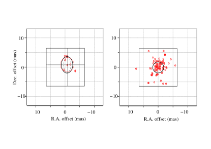
3.3 Derivation of the Positions and the Orbits
The procedure described above allows us to derive the stellar positions and the infrared position of Sgr A* with respect to the radio rest frame. We choose only images (33 in total) in which Sgr A* was flaring in the infrared in order to locate it directly in our coordinate system and have a good control of its possible motion with respect to the stellar cluster. In addition to the three candidate stars (S2, S38, and S55/S0-102), five stars (S7, S10, S26, S30, and S65) in their vicinity of them are selected to verify their reported positions and motions (Gillessen et al., 2009b; Plewa et al., 2015; Gillessen et al., 2017). This allowed us to validate the quality of the reference frame on an image-by-image basis. These reference stars are chosen from the bright sources within the central arcsecond and have relatively low velocities and almost linear motions on the sky. Moreover, they can always be detected without any confusion or overlapping with other sources.
After locating all sources in all images, the pixel positions of the three candidate stars and five reference stars are extracted. This is done by two-dimensional Gaussian fits of the position of the isolated sources. In the case of partial overlapping of stars in some epochs, the pixel positions are obtained without Gaussian fit, and therefore larger corresponding measurement errors are considered.
S2 can be detected in all 33 images from 2002 to 2015. S38 is probably confused with other sources in the years before 2004 and thus we keep only 29 astrometric measurements from 2004 to 2015 for it. Also S55/S0-102 is a faint star (16 times fainter than S2; Meyer et al., 2012) located in a very crowded region close to Sgr A*, therefore it is not detectable in every image, and that leaves us with 25 measurements from 2004 to 2015.
The pixel positions are transformed into an astronomic reference frame. To do so, we fit a linear equation of motion to the five reference stars, given in Table 2, and find the residuals in all the mosaics. We use the mean of all the residuals from all the reference stars in the image to correct for the image distortion and the astronomic positions of all our sources including Sgr A* in each corresponding image. The standard deviation of the mean of the residuals is inserted into the uncertainties of the astrometric data as the uncertainty of the reference frame. The resulting positions are given in Tables 3–5 for S2, S38, and S0-102/S55, respectively. Fitting a linear motion to the Sgr A* data after these transformations, we get
| (5) |
| Star | R.A. | Dec. | |
|---|---|---|---|
| (yr) | (arcsec) | (arcsec) | |
| S7 | 2002.578 | (0.5146 0.0026)+(-0.0040 0.0001)t | (-0.0421 0.0020)+(-0.0016 0.0002)t |
| S10 | 2002.578 | (0.0552 0.0023)+(-0.0045 0.0001)t | (-0.3736 0.0020)+(0.0037 0.0002)t |
| S26 | 2002.578 | (0.5105 0.0027)+(0.0060 0.0001)t | (0.4296 0.0020)+(0.0016 0.0004)t |
| S30 | 2002.578 | (-0.5434 0.0024)+(-0.0001 0.0003)t | (0.3806 0.0021)+(0.0036 0.0002)t |
| S65 | 2002.578 | (-0.7575 0.0034)+(0.0023 0.0006)t | (-0.2684 0.0033)+(-0.0015 0.0006)t |
| Date | R.A. | Dec. | R.A. Error | Dec. Error |
|---|---|---|---|---|
| (Decimal) | (arcsec) | (arcsec) | (arcsec) | (arcsec) |
| 2002.578 | 0.0386 | 0.0213 | 0.0066 | 0.0065 |
| 2003.447 | 0.0385 | 0.0701 | 0.0009 | 0.0010 |
| 2003.455 | 0.0393 | 0.0733 | 0.0012 | 0.0012 |
| 2004.511 | 0.0330 | 0.1191 | 0.0010 | 0.0008 |
| 2004.516 | 0.0333 | 0.1206 | 0.0009 | 0.0006 |
| 2004.574 | 0.0315 | 0.1206 | 0.0009 | 0.0009 |
| 2005.268 | 0.0265 | 0.1389 | 0.0007 | 0.0011 |
| 2006.490 | 0.0141 | 0.1596 | 0.0065 | 0.0065 |
| 2006.584 | 0.0137 | 0.1609 | 0.0033 | 0.0007 |
| 2006.726 | 0.0129 | 0.1627 | 0.0033 | 0.0007 |
| 2006.800 | 0.0107 | 0.1633 | 0.0033 | 0.0007 |
| 2007.205 | 0.0064 | 0.1681 | 0.0004 | 0.0007 |
| 2007.214 | 0.0058 | 0.1682 | 0.0004 | 0.0008 |
| 2007.255 | 0.0069 | 0.1691 | 0.0010 | 0.0007 |
| 2007.455 | 0.0047 | 0.1709 | 0.0004 | 0.0006 |
| 2008.145 | -0.0076 | 0.1775 | 0.0007 | 0.0012 |
| 2008.197 | -0.0082 | 0.1780 | 0.0007 | 0.0011 |
| 2008.268 | -0.0084 | 0.1777 | 0.0006 | 0.0008 |
| 2008.456 | -0.0118 | 0.1798 | 0.0006 | 0.0009 |
| 2008.598 | -0.0126 | 0.1802 | 0.0009 | 0.0010 |
| 2008.708 | -0.0127 | 0.1806 | 0.0008 | 0.0013 |
| 2009.299 | -0.0216 | 0.1805 | 0.0006 | 0.0009 |
| 2009.334 | -0.0218 | 0.1813 | 0.0006 | 0.0009 |
| 2009.501 | -0.0233 | 0.1803 | 0.0005 | 0.0008 |
| 2009.605 | -0.0266 | 0.1800 | 0.0012 | 0.0015 |
| 2009.611 | -0.0249 | 0.1806 | 0.0006 | 0.0008 |
| 2009.715 | -0.0260 | 0.1804 | 0.0006 | 0.0008 |
| 2010.444 | -0.0347 | 0.1780 | 0.0013 | 0.0021 |
| 2010.455 | -0.0340 | 0.1774 | 0.0008 | 0.0013 |
| 2011.400 | -0.0430 | 0.1703 | 0.0009 | 0.0017 |
| 2012.374 | -0.0518 | 0.1617 | 0.0012 | 0.0016 |
| 2013.488 | -0.0603 | 0.1442 | 0.0006 | 0.0019 |
| 2015.581 | -0.0690 | 0.1010 | 0.0014 | 0.0010 |
| Date | R.A. | Dec. | R.A. Error | Dec. Error |
|---|---|---|---|---|
| (Decimal) | (arcsec) | (arcsec) | (arcsec) | (arcsec) |
| 2004.511 | -0.0667 | 0.0576 | 0.0017 | 0.0016 |
| 2004.516 | -0.0673 | 0.0690 | 0.0066 | 0.0065 |
| 2005.268 | -0.1178 | 0.0583 | 0.0065 | 0.0066 |
| 2006.490 | -0.1544 | 0.0558 | 0.0065 | 0.0065 |
| 2006.584 | -0.1600 | 0.0613 | 0.0073 | 0.0078 |
| 2006.726 | -0.1684 | 0.0550 | 0.0009 | 0.0008 |
| 2006.800 | -0.1690 | 0.0549 | 0.0011 | 0.0009 |
| 2007.205 | -0.1851 | 0.0513 | 0.0005 | 0.0008 |
| 2007.214 | -0.1853 | 0.0506 | 0.0005 | 0.0008 |
| 2007.255 | -0.1807 | 0.0524 | 0.0010 | 0.0007 |
| 2007.455 | -0.1898 | 0.0474 | 0.0005 | 0.0065 |
| 2008.145 | -0.2058 | 0.0363 | 0.0009 | 0.0013 |
| 2008.197 | -0.2065 | 0.0359 | 0.0008 | 0.0011 |
| 2008.268 | -0.2049 | 0.0338 | 0.0007 | 0.0009 |
| 2008.456 | -0.2111 | 0.0325 | 0.0008 | 0.0010 |
| 2008.598 | -0.2141 | 0.0346 | 0.0010 | 0.0010 |
| 2008.708 | -0.2175 | 0.0338 | 0.0010 | 0.0013 |
| 2009.299 | -0.2315 | 0.0244 | 0.0007 | 0.0009 |
| 2009.334 | -0.2310 | 0.0241 | 0.0007 | 0.0009 |
| 2009.501 | -0.2344 | 0.0216 | 0.0006 | 0.0008 |
| 2009.605 | -0.2360 | 0.0156 | 0.0012 | 0.0015 |
| 2009.611 | -0.2350 | 0.0202 | 0.0007 | 0.0008 |
| 2009.715 | -0.2363 | 0.0178 | 0.0006 | 0.0009 |
| 2010.444 | -0.2415 | 0.0053 | 0.0013 | 0.0021 |
| 2010.455 | -0.2437 | 0.0009 | 0.0009 | 0.0014 |
| 2011.400 | -0.2425 | -0.0113 | 0.0010 | 0.0017 |
| 2012.374 | -0.2519 | -0.0251 | 0.0013 | 0.0017 |
| 2013.488 | -0.2450 | -0.0409 | 0.0007 | 0.0019 |
| 2015.581 | -0.2320 | -0.0617 | 0.0016 | 0.0013 |
| Date | R.A. | Dec. | R.A. Error | Dec. Error |
|---|---|---|---|---|
| (Decimal) | (arcsec) | (arcsec) | (arcsec) | (arcsec) |
| 2004.511 | 0.0549 | -0.1552 | 0.0066 | 0.0065 |
| 2004.516 | 0.0711 | -0.1536 | 0.0066 | 0.0065 |
| 2005.268 | 0.0707 | -0.1437 | 0.0065 | 0.0066 |
| 2006.490 | 0.0731 | -0.1199 | 0.0065 | 0.0065 |
| 2006.584 | 0.0749 | -0.1220 | 0.0065 | 0.0065 |
| 2006.726 | 0.0790 | -0.1180 | 0.0066 | 0.0065 |
| 2006.800 | 0.0731 | -0.1169 | 0.0066 | 0.0065 |
| 2007.205 | 0.0835 | -0.0883 | 0.0065 | 0.0065 |
| 2007.255 | 0.0797 | -0.0763 | 0.0066 | 0.0065 |
| 2007.455 | 0.0784 | -0.0635 | 0.0065 | 0.0065 |
| 2008.145 | 0.0659 | -0.0346 | 0.0065 | 0.0066 |
| 2008.197 | 0.0641 | -0.0338 | 0.0065 | 0.0066 |
| 2008.268 | 0.0711 | -0.0309 | 0.0065 | 0.0066 |
| 2008.456 | 0.0692 | -0.0167 | 0.0065 | 0.0066 |
| 2008.598 | 0.0678 | -0.0144 | 0.0066 | 0.0066 |
| 2008.708 | 0.0620 | -0.0058 | 0.0066 | 0.0066 |
| 2009.334 | -0.0017 | 0.0358 | 0.0065 | 0.0066 |
| 2009.501 | -0.0257 | 0.0291 | 0.0065 | 0.0066 |
| 2009.605 | -0.0305 | 0.0243 | 0.0066 | 0.0067 |
| 2009.715 | -0.0390 | 0.0378 | 0.0065 | 0.0066 |
| 2010.444 | -0.0620 | -0.0453 | 0.0066 | 0.0068 |
| 2010.455 | -0.0523 | -0.0404 | 0.0018 | 0.0020 |
| 2011.400 | -0.0492 | -0.1080 | 0.0066 | 0.0067 |
| 2012.374 | -0.0345 | -0.1180 | 0.0013 | 0.0029 |
| 2013.488 | -0.0134 | -0.1380 | 0.0007 | 0.0019 |
| 2015.581 | 0.0239 | -0.1678 | 0.0016 | 0.0066 |
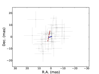
Figure 2 shows this linear fit compared to the previous study done by Gillessen et al. (2009b). The linear fits and the uncertainties of the fits were done with a bootstrap algorithm in which we generate 50 random samples with replacements of size equal to the observed dataset and calculate the statistics on the sampling distribution.
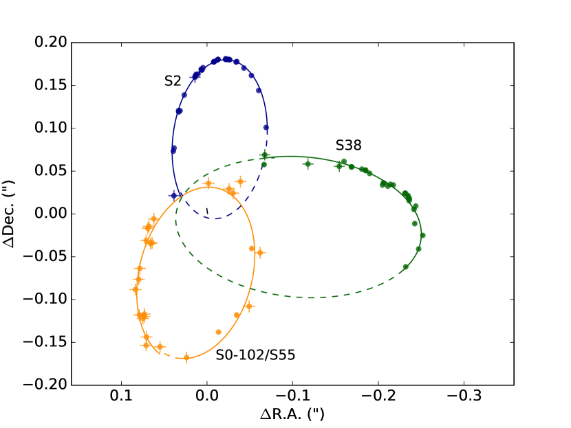
We use the PN approximation discussed in Sect. 2.2 and fit our astrometric data for the candidate stars (and simultaneously for the radial velocity in the case of S2 and S38) to the relativistic model using the minimum method. The measurement errors (considering both astrometric errors and reference frame errors) are scaled in a such way that the reduced = 1. The result is shown in Fig. 3 for all candidate stars.
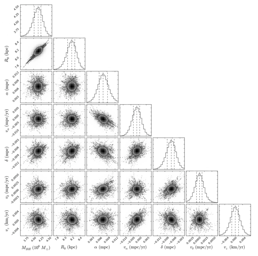
Moreover, we run Markov Chain Monte Carlo (MCMC) simulations using Newtonian models to find all six orbital parameters for the candidate stars and the gravitational potential parameters of the SMBH (including its mass and the distance to the GC), and their 1 uncertainties simultaneously. We use emcee by Foreman-Mackey et al. (2013), which is an affine-invariant ensemble sampler for MCMC. We repeat the simulations using one (S2), two (S2 and S38), and three (S2, S38, and S55/S0-102) stars. Figure 4 is a part of the results for such a simulation. The rest of the parameters are omitted for reasons of legibility. The histograms along the diagonal are the marginalized distribution for each parameter and resemble normal distributions. The rest of the panels show 2D cuts of the parameter space. If the posterior probability is broad then that parameter is not well constrained. However, the posterior probability is compac,t which means all parameters are well constrained. There are some correlations between the parameters, especially between and .
We change the model afterwards to a relativistic one using Equation (1) and repeat the simulations for the same combinations of the candidate stars. The results from all MCMC simulations are given in Table 6. The errors of the parameters are the result of their distributions from the MCMC simulations. Using two and three candidate stars reduces the uncertainties in determining most of the parameters, especially the velocity of Sgr A*, as a result of the lack of astrometric data in the lower part of the orbit of S2 and S38. Moreover Zucker et al. (2006) indicate that using a Keplerian model instead of a relativistic one might systematically underestimate .
| Keplerian | Relativistic | |||||
|---|---|---|---|---|---|---|
| Parameter (unit) | S2 Only | S2, S38 | S2, S38, S55/S0-102 | S2 Only | S2, S38 | S2, S38, S55/S0-102 |
| Black hole: | ||||||
| (106 ) | ||||||
| Distance (kpc) | ||||||
| (mas) | ||||||
| (mas) | ||||||
| (mas yr-1) | ||||||
| (mas yr-1) | ||||||
| (km s-1) | ||||||
| S2: | ||||||
| () | ||||||
| () | ||||||
| () | ||||||
| () | ||||||
| (yr) | ||||||
| S38: | ||||||
| () | ||||||
| () | ||||||
| () | ||||||
| () | ||||||
| (yr) | ||||||
| S55/S0-102: | ||||||
| () | ||||||
| () | ||||||
| () | ||||||
| () | ||||||
| (yr) |
For the starting point of the MCMC simulations, first we minimize the for the orbital parameters (the position and velocity for the relativistic model at the reference epoch) and only the mass of the SMBH and the distance to the GC. Then we try to improve the resulting by setting the position and the velocity of the central mass as free parameters. The results are then used in the code for MCMC simulations. The reference epoch for the relativistic fits is 2002 April and that for the Newtonian fits is 2002 July. This needs to be considered when comparing the position of the BH at the reference epochs of the two models.
4 Simulations and Case Studies
4.1 The Case of Simulated Stars within the Orbit of S2
The orbits of 14 stars (see Table 7) are generated using Equation (2) by positioning them at different apoapse distances with different velocities within the orbit of S2 and integrating the equation of motion using the fourth-order Runge–Kutta method until the next apoapse is reached. Since the eccentricity of the orbit is not one of the initial parameters, an additional parameter is introduced that has a linear correlation with the eccentricity in order to be able to generate orbits with the same eccentricity. If the total energy does not remain constant, the orbit gets stretched over time and the next apoapse will not be equal to the first one; consequently the resulting orbit will fail to be suitable for the purpose of this study. Hence, in order to keep the energy constant to a desirable approximation for the first few orbits, the time steps are taken to be relatively small. The drift motion of the BH can potentially have a large effect on the simulated orbits, but small orbits with short orbital periods have the advantage of being immune to the possible effects of the motion of the central mass.
Also we assume that each S-star is a single star and not a binary or a bright component of one. Binaries can have effects on astrometric and radial velocity measurements and the binary disruption at the periapse can affect the orbit of the primary. Moreover there is no evidence, at least for S2, of a secondary component in the spectra (Eisenhauer et al., 2005; Martins et al., 2007, 2008).
| Star | R.A. | ( , ) | ||||||
|---|---|---|---|---|---|---|---|---|
| (mpc) | (103km s-1) | (mpc) | (mpc) | (rad) | ||||
| 1 | 0.07 | (5.34 , 0.00) | 0.120 | |||||
| 2 | 0.5 | (2.00 , 0.00) | 0.015 | |||||
| 3 | 0.05 | (7.75 , 0.00) | 0.106 | |||||
| 4 | 0.06 | (7.07 , 0.00) | 0.087 | |||||
| 5 | 0.04 | (10.00 , 0.00) | 0.095 | |||||
| 6a | 0.06 | (6.45 , 5.00) | 0.061 | |||||
| 6b | 0.06 | (8.16 , 0.00) | 0.061 | |||||
| 7a | 0.05 | (8.00 , 6.00) | 0.056 | |||||
| 7b | 0.05 | (10.00 , 0.00) | 0.056 | |||||
| 8 | 0.07 | (8.45 , 0.00) | 0.039 | |||||
| 9 | 0.10 | (7.07 , 0.00) | 0.027 | |||||
| 10 | 0.05 | (10.95 , 0.00) | 0.044 | |||||
| 11a | 0.06 | (8.00 , 6.00) | 0.037 | |||||
| 11b | 0.06 | (10.00 , 0.00) | 0.037 | |||||
| 12 | 0.08 | (9.35 , 0.00) | 0.022 | |||||
| 13 | 0.09 | (9.43 , 0.00) | 0.017 | |||||
| 14 | 1.00 | (3.00 , 0.00) | 0.001 | |||||
| S2 | - | - | 0.0007 |
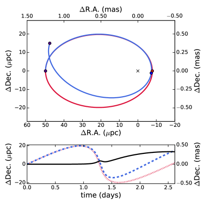
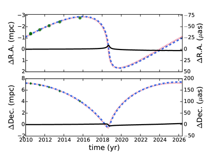
Figure 5 demonstrates two different paths a star (case 7a of Table 7) will take with the same initial position and momentum, on the sky plane, when the orbit is purely Newtonian (red line) and when the first-order PN approximation is used. The blue/red circle shows the periapse position of the relativistic/Newtonian orbit. The purple points mark the positions of the apoapses for both orbits. For a Newtonian orbit the apoapse positions overlap, while for a relativistic orbit there is a shift in the apoapse position after one orbit. The orbit is oriented horizontally so most of the difference between the positions can be seen in the declination (Dec.) direction. The Dec. of the two orbits, the dashed blue line for the relativistic orbit and the dotted red line for the Newtonian, and the difference between them, the solid black line are plotted against time in the bottom panel. As a result of the periapse shift, most of the deviation from the Newtonian orbit happens after the periapse. There is a peak in the plot, which indicates the periapse.
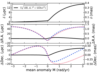
However, if one wants to compare the orbits at the same phase one should plot the positions against the mean anomaly. The middle and bottom panels in Fig. 6 show the R.A. and Dec. of the relativistic orbit with a dashed blue line and those of the Newtonian with a dotted red line with respect to their mean anomaly in units of rad yr-1. The difference between the two lines in each panel is shown with a solid black line. The top panel depicts the distance between the positions of the two cases, defined as . From one apoapse to the next the mean anomaly changes in the range M . The periapse happens at . There is no peak in the plot showing the difference in the Dec., since the two periapses happen at the same mean anomaly but not at the same time.
As mentioned above, since all our simulated orbits are located inside the orbit of S2, the upper limit for selecting the simulated case studies is the apoapse distance of S2 ( 0.234). We disregard the orbits with periapse distances smaller than the tidal disruption radius near Sgr A*, since main-sequence stars such as S-stars cannot exist within this radius. The tidal radius for the stars in the GC is defined as 85 as, given by Alexander (2005) for a star of mass , a radius of , and a SMBH mass of = 3.5 106 . The mass of the SMBH is estimated to be 4.3 106 in this study, thus the tidal radius is 90 as.
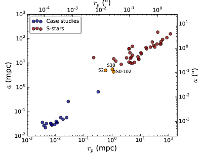
The distribution of these simulated stars compared to the distribution of the detected S-stars is depicted in Fig. 7. The S-stars are shown with red circles while the simulated stars are shown with blue circles in the plots of semimajor axis versus eccentricity (top panel) and semimajor axis versus periapse distance (bottom panel). S2, S38, and S55/S0-102 are shown with orange circles and labelled.
The stars for our highly relativistic case studies cover a similar range in eccentricity to the S-stars but smaller orbital axes. With this coverage we start developing a method to estimate and predict how relativistic the orbits of stars are after observing them for just one orbit using only astronomical data. We should keep in mind that our main goal is to find a correlation between the theoretical relativistic and the observational parameters.

4.2 Developing methods to measure the PN effects
To develope a method to measure the strength of the PN effects, first we have to find an observable that is relatively easy to measure and that changes noticeably as a result of these effects. In the search for such an observable, which also enables us to exploit the uncertainties in the orbital fitting, we employ a concept similar to that of the squeezed states.
4.2.1 Squeezed States
In our framework of orbital fitting we consider a squeezed state to be any state in which an uncertainty principle is fulfilled and saturated. As a precondition for this, we need the product of two quantities and to be larger than but very close to a minimum limit
| (6) |
In this context the term uncertainty implies that the fitting procedure allows a considerable portion of the measurement uncertainties to be shifted back and forth between the two quantities. Then we consider the result of the fitting procedure to be a state that allows us to squeeze the uncertainties into one of the variables.
If we set = and = with being the weighted sum of the squared errors as a result of fitting an elliptical orbit to the observational data, then e describes the goodness of the fit or its likelihood of representing the orbit well. The subscripts u and l in this paper denote the upper and lower parts of the orbit respectively. Hence, we write
| (7) |
or
| (8) |
We can now separate the fitting errors contributed by the random uncertainties of the measurement (subscript r) and those contributed by the misfit of the orbital shape if it is not a perfect ellipse (subscript s). The inequality (8) is true (i.e. the inequality sign is justified) if we set , which describes the overall goodness of the combined upper and lower orbital fit just based on the random measurement uncertainties, so
| (9) |
The inequality is largely compensated for if we include on the right side of the equation the goodness of the combined upper and lower orbital fit just based on the mismatch of the overall orbital shape:
| (10) |
If we assume that the measurement uncertainties for the upper and lower parts of the orbit are similar, , then we can write
| (11) |
For a global fit to the entire orbit the uncertainties are distributed well between the upper and lower parts of the orbit, and we assume that the measurement uncertainties are similar, :
| (12) |
However, if we exclusively fit the lower or upper part of the orbit well, the situation changes. If the measurements are very precise then on one side the uncertainties due to the mismatch of the shape may become dominant and much larger than the random uncertainties. As can be seen in Figs. 8 and 9 this may be relevant the for relativistic orbits. In this case, the ellipses fitted to the lower part of the orbit have systematically lower ellipticities and semimajor axes. If fitting one side only, the uncertainties due to a mismatch of the orbital shape will be concentrated (squeezed) to the orbital section on the opposite side and we find
| (13) |
| (14) |
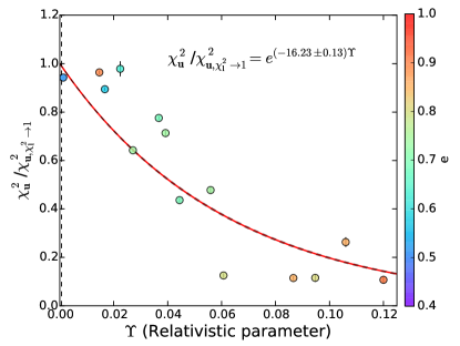
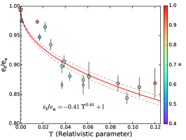
Here, and are the squeezed -values one obtains after the fit to only one side of the orbit. Therefore, the ratio between or and these two quantities can be used to decide on the degree to which the orbit is dominated by relativistic effects. Figure 10 demonstrates the correlation between and one of these ratios () for the cases in Table 7. If then we expect 1/2 for the ratio (equation (13)), but for more relativistic cases gets even larger than . As we go to more Newtonian cases, the ratio approaches unity since the systematic differences between the upper and the lower parts of the orbit disappear. The best fit describing the correlation is
| (15) |
However, squeezing the goodness of fit to only one side of the orbit has consequences for the orbital elements. For an ellipse we know
| (16) |
where is the eccentricity, is the semimajor axis,and is the semiminor axis of the ellipse. Equation (16) shows that deviations of the overall orbital shape from an ellipse will become apparent in the misfit of the semimajor axis and eccentricity if we fit only to the lower or upper half of the orbit, respectively. Such deviations from Newtonian ellipses are expected if the orbits are influenced by relativistic effects or by an additional smooth or granular extended mass distribution. The differences can be expressed as ratios of parameters and . Here, the subscripts again indicate for which orbital section the fit was optimized.
The method we present can be compared to a method by Angélil & Saha (2014) to show the relativistic effects on the argument of the periapse . The predicted pericenter shift for S2 during its Sgr A* flyby in 2018 will amount to about 11′ (for a semimajor axis of 0″.126, an eccentricity of 0.88, and a BH mass of 4.15 106 ), but Angélil & Saha (2014) point out that it does not occur smoothly. They find that the difference in from the pre- to post-periapse part of the orbit occurs almost in a step at each pericenter passage. This method is basically equivalent to a measurement of the periapse shift using the two halves of the orbit before and after the periapse.
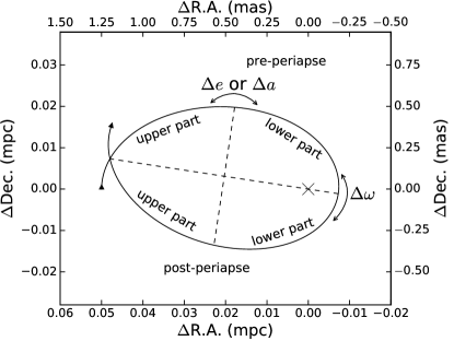
With the ratios and our method uses the orbital differences in the radial direction (see Fig. 8) and we exploit the folding symmetry along the semiminor axis (as expected from a Newtonian motion) while Angélil & Saha (2014) make use of the folding symmetry of the orbit along the semimajor axis. Hence, their method corresponds to squeezing the goodness of the orbital fit to the pre-/post-periapse part of the orbit (Fig. 8) and therefore can also be described using the formalism we present here.
The rapid change of can in principle be derived using only small sections of the pre-/post-periapse part of the orbit. However, one still needs the information on the full orbit, because the orbital solutions need to be derived in the same orbital plane in order to represent the progressing periapse shift precisely. Using elliptical fits to all or most of the upper/lower or pre-/post-periapse part of the orbit, we ensure that the entire orbit within its plane is represented in as complete a way as possible.
4.2.2 Comparison of Methods
In order to illustrate the method of and ratios and the method, we consider two full orbits of the case 7b from Table 7 (see Fig. 9). The apoapses and periapses are marked by blue and violet circles respectively in the left panel. The simulated data points shown with yellow circles make a full closed orbit on the sky in the middle panel. These data points are generated after equal time intervals. We fit an ellipse to the upper half of the data, shown as a red solid ellipse in the right panel. Subsequently, we fit another ellipse to the lower half of the data, shown as a cyan solid ellipse in the same panel.

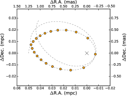
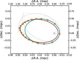
We repeat these steps for all our case studies and report the different values for the semimajor axis and eccentricity of the two halves in columns 5–8 of Table 7. The elliptical orbits and the orbital elements are obtained by a fit to the data points using the L-BFGS-B (limited-memory Broyden–Fletcher–Goldfarb–Shanno) minimization method. In order to estimate a value for the uncertainty of the measurement of each data point in the fits, we use the standard deviation of all the upper or lower half of the data points considering no mean displacement from a Newtonian orbit for half of the orbit, and an approximate mean displacement of /4 for the other half. Here is the periapse shift. The uncertainties include misfitting ellipses to the upper and lower parts of the orbit. The time intervals between the data points are in accordance with the scale of the orbit and consequently its orbital period, which can be between an hour and a month.
Next, we apply the method discussed in Sect. 4.2.1 by fitting ellipses to the pre- and post-periapse halves of the orbits of the case studies. This method is illustrated for the case 7b from Table 7 in Fig 11. We get the same values for all the orbital elements except the argument of the periapse for the two fits, as expected. The difference in of the two halves for each case study is reported in the last column of Table 7.
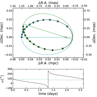
Without loss of generality all our case studies are located on the sky plane, i.e. they have no velocity component in the direction. For the sake of completeness, we add a velocity component to three of the case studies and consequently generate three cases with inclination (6a, 7a, and 11a in Table 7). Applying the two methods to these cases, assuming a real situation in which we do not have any information about the inclination but the radial velocity, includes a few more steps. Before fitting the ellipses for each of them we first have to fit a simple Newtonian orbit to the astrometric and radial velocity data to find the inclination and the line of nodes of the orbit. Then using the inclination and the argument of the periapse we have to correct the astrometric data for inclination. Afterwards we can continue with the rest of the steps. However, as a consequence of these additional steps, we have additional sources of uncertainty. Therefore, we choose not to use these cases for our analysis.
4.3 The case of S2
To see how well the methods work, we apply them to the data of one full S2 orbit. Since our VLT data from 2002 to 2015 do not allow us to cover one full orbit and since we lack sufficient data on the lower half of the orbit, we add the data provided by Boehle et al. (2016) from 1995 to 2010 to the data presented in this work. However, the two data sets do not share the same reference coordinate system. We use the approach discussed in Gillessen et al. (2009a) to bring the two data sets into a single coordinate system by assuming that they differ only in the position of the origin and the zero velocity. Therefore, we add four additional parameters—, , , and —to our parameters. Also, we make use of the PN approximation and the astrometric data presented here and in Boehle et al. (2016), and the radial velocity data in the latter and in Gillessen et al. (2009a). Finally we fit simultaneously for the S2 orbital parameters, the gravitational potential parameters, and the new parameters to bring the two data sets into a single coordinate system. The fit results for these four new parameters are
| (17) |
These values refer to the epoch of 1995 May, which is chosen as the zero time of the orbital fit. The uncertainties are the results of MCMC simulations. Using these parameters and applying them on the data from Boehle et al. (2016), we have sufficient data covering all quarters of the orbit to apply the two methods to S2. The resulting semimajor axis, eccentricities, and for S2 using the two methods are in the last row of Table 7.
Figure 12 compares the Newtonian (dotted red) and relativistic (dashed blue) fits to the combined data of S2 from 1995 to 2015. It shows the difference between the two models (black solid line) in the current period and indicates that the difference will manifest itself especially during and after the periapse in 2018.
Although Gillessen et al. (2009a) reject the probability of a rotation between the VLT and Keck data sets and we follow their suggested approach in Sect. 4.3 for bringing the two data sets into one coordinate system, adding a parameter for rotation in our calculation in order to put a limit on a possible rotation is not entirely unjustifiable. Such a rotation (if it existed) can have an undesirable effect particularly on the derivation of of S2 in Sect. 4.3 for the reason that we used only the data provided by the Keck data set for the pre-periapse fit. As a result we performed a separate MCMC simulation in which we introduced a parameter in addition to our four initial parameters (, , , ) for describing the difference in the coordinate systems. Without loss of generality we implemented the center of rotation at the location of Sgr A* and looked for the possible value of for a Newtonian orbital fit to the combined S38 data using the data provided in Boehle et al. (2016) from 2004 to 2013. The perpendicular orientation with respect to S2 on the sky makes S38 ideal for testing for a rotation between the two data sets. Irrespective of the expected small periapse shift of the orbit of S38 of only about 6′, this source is ideally suited to probe relative rotations of the data set with respect to each other because the highest quality comparison data are all on the northern side, i.e., on a single side, of the orbit. We find an upper limit for the rotation of 0′.002 for the S38 orbital fit. If we repeat the procedure for the combination of the S2 and S38 data (again only on the sections of the orbits covered by both data sets) we find an upper limit on the rotation value of 0′.1. The expected periapse shift of S2 is about 11′ (for a semimajor axis of 0″.126, an eccentricity of 0.88, and a BH mass of 4.15 106 ). Since we regard the very small rotational values as upper limits we did not apply them and we continue the analyses with the results from the MCMC simulations described before. Thus we conclude that our combination of the two data sets is ideally suited to probing for relativistic effects on the orbital elements.
5 Results
5.1 The simulated case studies
A measure of the strength of the PN effects is the relativistic parameter at the periapse, (see also Alexander, 2005; Zucker et al., 2006; Ghez et al., 2008). Other suggested parameters are the dimensionless periapse distance, the periapse shift, and the speed at the periapse in units of the speed of light , with being the velocity during the closest approach to the BH (Zucker et al., 2006). It is a justifiable parameter for determining the approximate magnitude of the components of the Schwarzschild metric outside a single object in vacuum (Baker et al., 2015). is by definition dependent on the orbital shape, i.e. the semimajor axis and eccentricity. The inverse correlations between and the semimajor axis (and consequently the orbital period) and the eccentricity are demonstrated in Fig. 13. The solid lines are = 0.9–0.5 from top to bottom in the left panel, and = 0.02–0.06 mpc (0.5–1.5 mas), = 0.27 mpc (6.7 mas), = 1 mpc (25 mas), and = 5 mpc ( 125 mas) from top to bottom in the right panel. The circles represent the simulated stars in the plane of the sky and the diamonds show the simulated stars with inclinations (corrected for) with respect to the sky plane, listed in Table 7. The dashed line shows the of S2 for both panels, which is the minimum in this study.
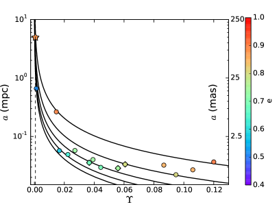
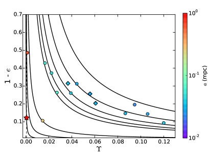
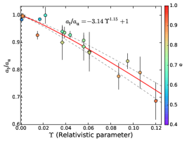
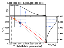
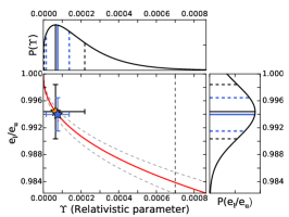
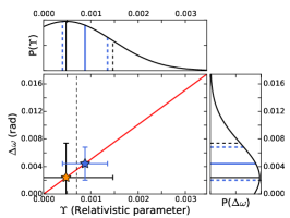
The PN effects should depend only on , according to the strong equivalence principle. However, this is not the case for other theories of gravitation so one should investigate the dependence of these effects on multiple parameters (Zucker et al., 2006). In this study our main candidate for a parameter that can describe the strength of the PN effects in an orbit is . Figure 14 shows the correlation between and ratios of the orbital parameters and , as described in Sect. 4 for the stars in Table 7.
As a result of the dependence of on the eccentricity and the semimajor axis , one might expect that in order to find a clear correlation between and the ratios and (see Fig. 13), a parameterization is necessary. It can be understood from Fig. 13 and from the definition of that the effects of and on are only dominant on small scales and for large eccentricities. These effects are negligible for sufficiently large orbits with low eccentricities. If we consider that the eccentricity of the stellar orbits typically ranges between 0.4 and 0.9 then this will result in a variation of by a factor of 6. The possible semimajor axis for orbits with between the tidal disruption radius and of S2 ranges between 0.01 mpc (0.025 mas) and 5 mpc (125 mas). For changes in semimajor axis between these values, varies by a factor of 500. However, in the ratios and their dependences on and , respectively, cancel out almost entirely. As a result, the correlations between and the two ratios in Fig. 14 show only a little scatter of the data around the calculated curves.
Figure 14 shows that the ratios and get smaller as the orbit gets more relativistic (i.e. increases). This means that, for all relativistic orbits, the fit to the upper half has a larger semimajor axis and is more eccentric than the fit to the lower half, as expected. Also, as goes to zero, both ratios approach unity since less and less deviation from a Newtonian orbit is anticipated. The best fits after trying a few models to describe the correlations are
| (18) |
and
| (19) |
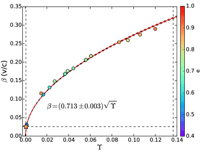
Using the periapse distance instead of the relativistic parameter will not give us any new information, since . According to Zucker et al. (2006), the stars with smaller periapse passages and consequently larger velocities at the periapse, i.e. larger , are in orbits with stronger PN effects. Also, for highly eccentric orbits with and 1 (approximately Newtonian), Zucker et al. (2006) show . Here, we also find as can be seen in Fig. 15.
5.2 The Case of S2
We also apply the analysis to data on the S-star S2. The orbit of this star shows the highest ellipticity and gives us a chance of deriving the relativistic parameter. The results for and e from the fits to the upper and lower halves of the combined data set of S2, given in the last row of Table 7, are the mean and standard deviation of the assumed normal distributions from the MCMC simulations. However, when calculating and , since both ratios in the derived correlation are limited to 1 (Equation (18) and (19)), we choose to use a truncated normal distribution as the probability density function (pdf) given by
| (20) |
for with being the pdf of a standard normal distribution and being the cumulative distribution function. Using a change of variables and the correlations between the observable parameters and , we can obtain the pdf of . These pdfs are shown next to the - and -axis in the bottom panels of Fig. 14 for S2. The solid black and dashed lines are the means and standard deviations, respectively. They correspond to the orange stars in all three panels. Moreover the medians and the median absolute deviations (”mad”) are shown with blue solid and dashed lines, respectively. They correspond to the blue stars with their error bars representing the ”mad”. The median and mean values are listed in Table 8.
| Method | Mean | Median | |||
|---|---|---|---|---|---|
| With the drift | |||||
| motion of BH: | |||||
| (Mean) | 0.00193 0.00432 | 0.00006 0.00015 | 0.00048 0.00099 | 0.00074 0.00227 | – |
| (Median) | 0.00405 0.00199 | 0.00008 0.00006 | 0.00088 0.00048 | ||
| Without the drift | |||||
| motion of BH: | |||||
| (Mean) | 0.00179 0.00424 | 0.00001 0.00005 | 0.00048 0.00099 | 0.00069 0.00223 | – |
| (Median) | 0.00392 0.00194 | 0.00002 0.00002 | 0.00088 0.00048 | 0.00142 0.00102 | 0.00088 0.00086 |

The strongest cumulative relativistic effect is the shift of the periapse due to a Schwarzschild black hole up to the first order and is given by
| (21) |
per orbit. Hence, for the second method explained in the previous section ( method), we can repeat the approach explained above. Once more the relation (Equation (21)) is limited only to the positive values for . Therefore to obtain the pdf of we use the truncated pdf of as shown in the top left panel of Fig. 14. The results are presented in Table 8. Since the values for S2 from and both describe the case for folding symmetry along the semi-minor axis, we averaged their results. Consequently, the final mean value of S2 is obtained by averaging the values corresponding to the orthogonal folding symmetries. The three values obtained for S2 are obtained from methods that react on statistical and systematic uncertainties of the data in different ways. The variations that affect act differently on the ellipticity and the semi-major axis. Similarly, the variations that affect the semi-major axis may not result in a change in . Hence, the uncertainties between the three different methods certainly do not follow a Gaussian distribution. Therefore, the three values need to be combined by averaging the median and ”mad” rather than the mean and standard deviation.
For a full treatment of S2 the drift motion of the central mass needs to be taken into account. This motion should be added to the coordinates of the ellipse we are fitting at each time step. Alternatively, the motion can be removed from the data points. If we consider the motion from Table 6 for the relativistic fit to only S2 data and remove it from the combined data set of S2, we get similar results as can be seen in Table 8.
5.3 Robustness of the Result
We can address the robustness of the result in different ways. First we exclude the possibility that the result is dominated by noise or by a drift motion of Sgr A*, then we highlight again that it is not due to rotation between the VLT and Keck data sets.
We assume that the orbital measurements are completely dominated by the noise and that the signal showing the variations of the orbital elements is dominated by noise. For simplicity we consider a displacement of an orbital section from the noise-unaffected orbit due to noise as a single degree of freedom. One can ask the question: how likely is it to get consistent results as presented in this section assuming that the noise contributions of the upper and lower halves and the pre- and post-periapse halves of the orbit are independent? Furthermore, we consider the collective noise contribution in each one of these quadrants as a displacement along the semimajor or semiminor axis of a single orbit. While no significant net displacement will occur for most of the noise realizations, a certain fraction of these realizations will result in such a displacement. Hence, the probabilities derived below are crude lower limits if one seeks to explain the result as being due to the noise only. Considering only the fraction of the noise realizations that result in a net displacement we have a total of 44 = 256 possibilities to combine them. Only one combination gives a unique configuration that results in the measured changes of , and the ratios and . This corresponds to a probability of 0.004, i.e., a 0.4% chance that the result is reproduced by noise-dominated measurements.
Allowing for at least one quadrant to be displaced improperly leaves us with five combinations that are consistent with the observed signal. Allowing for more than one of the four quadrants to be displaced improperly gives an inconsistent result for at least one of the quantities, , , or . Hence, there is only a 2% probability (5/256 = 0.019) that the result can be obtained serendipitously as a consequence of dominant noise. Therefore, we consider it to be highly unlikely that the common systematic tendency of the change in the orbital parameters and hence the corresponding ranges for the relativistic parameter are the result of pure noise only.
It can also be argued that the change in the orbital parameters is due to the drift motion of Sgr A*. In this case a constant shift in would be injected over the entire orbital time scale. For one orbit the drift would be of the order of , with being the semimajor axis of the orbit and the expected periastron shift. There would be no effect on for a north–south motion. However, in east–west direction a proper motion of Sgr A* of the order of 30 as yr-1 could explain the shift in . Nevertheless, by using the PN approximation for modeling the motion of S2 and correcting the orbital data for the residual drift motion before deriving the change in the orbital parameters, we can assume that it is very unlikely that the observed change in sign and magnitude of is due to the drift motion of Sgr A*.
It can also be excluded that the change in the orbital parameters is due to a relative rotation between the data sampling the pre- and post-periapse halves of the orbit. Both data sets are tied to the same VLA radio reference frame. Moreover the classical calibration of the camera rotation is better than 0.1, i.e. less than 6′, and therefore about a factor of two smaller than the expected periastron shift of about 11′ (for a semimajor axis of 0″.126, an eccentricity of 0.88, and a BH mass of 4.15 106 ). Furthermore, Plewa et al. (2015) find an upper limit on the temporal rotation of the infrared reference frame relative to the radio system of 7.0 as yr−-1 arcsec−-1. Over 20 yr this corresponds to an angle of less than 0′.5, i.e. 24 times smaller that the expected periastron shift. This is also consistent with our result from section 4.3. A comparison of the VLT and Keck data at times of equal coverage for S38 or for the combination of S2 and S38 results in an upper limit of the rotation of 0′.1, i.e., a value 110 times smaller than the expected periastron shift. Therefore, we consider it very unlikely that the observed change in sign and magnitude of is due to the effects of differential rotation.
6 Discussion
6.1 Comparison of the Results with the Literature
The next periapse passage of S2, assuming the values from simulations of all three stars with Newtonian models, is in 2018.51 0.22, which is in July. Boehle et al. (2016) have predicted it to be 2018.267 0.04, corresponding to April. In both cases the results indicate that the event might be optimally placed for observations. The upcoming event is highly anticipated since the deviations from a Newtonian orbit and the gravitational redshift are expected to be detectable as S2 goes through its closest approach. However, these tests of GR are possible only if we have a precise knowledge of the gravitational potential parameters and the orbit. Using the data from more than one star for orbital fitting is one way of getting a better precision in finding these parameters. Using multiple stars for determining MBH and R0 has been done before. Gillessen et al. (2017) find = (4.28 0.10) 106 and = 8.32 0.07 kpc for multiple-star fit. While the statistical uncertainties of these parameters are comparable to the uncertainties we report in our Newtonian multiple-star fit, the results reported by Gillessen et al. (2017) are in agreement with our values to within a 2 uncertainty (see Table 6). Similarly, Boehle et al. (2016) measurements from Keck are = (4.02 0.16) 106 and = 7.86 0.14 kpc. To within a 1 and 2 uncertainties, respectively, these quantities are in agreement with our comparable fit results (Newtonian S2 and S38). The uncertainties we obtain are very similar to those of Boehle et al. (2016).
The star S55/S0-102 was not selected before for mass and distance fits due to the lack of radial velocity data. Since we cannot constrain the Newtonian precession due to the uncertainty of the mass enclosed within the orbit of S2, we need at least one more star to measure the strength of the PN effects. S55/S0-102 has a very short orbital period and thus a large phase coverage. It has already passed through its periapse passage in 2009 and its next periapse time will be in 2021. Therefore, it is the best candidate for measuring deviations from a Newtonian orbit after S2. The parameters we derive for the Newtonian model using the combinations S2, S38, and S2, S38, S55/S0-102 give similar results within the uncertainties.
The estimates of mass and distance derived for the Newtonian and the relativistic models and being based solely on S2 give slightly higher results that are, however, within their larger uncertainties, still in agreement with the multiple-star solutions. They also agree very well with recent estimates of these quantities by Ghez et al. (2008) and Gillessen et al. (2009b) based on Newtonian solutions for S2 only.
Also the estimates of mass and distance for the S2, S38 combination in the relativistic case are in reasonable agreement with the Newtonian solutions, while these quantities are systematically larger in the relativistic case for the S2, S38, S55/S0-102 solution.
The ratios of the changes in orbital parameters of S2— and —and given in Table 7 agree with the study done by Iorio (2017) where time series of the first-order PN shifts of the osculating Keplerian orbital elements are found analytically and numerically. Iorio (2017) finds maximum shifts of = 30 au, = 0.003, and = 0.2 for S2. Considering a semimajor axis of = 0″.126 and an eccentricity of = 0.884, we get = 0.971 and = 0.997, which are in agreement with the values in Table 7. The results described by Iorio (2017) were obtained in a deductive way: a general relativistic theoretical scenario is used to deduce the orbital elements and their properties as a function of time, as one would expect them for the special star S2 close to the Sgr A* black hole. In our case we have to proceed in an inductive way. We start with positional and spectroscopic measurements of the three stars (including S2) that orbit the large mass associated with Sgr A*. The goal is to show that the orbit of S2 is significantly influenced by general relativistic effects. Hence, we have to provide an (indirect) observable that allows us to discriminate the relativistic from the nonrelativistic case, based on real data. The procedure we developed can be directly compared to and confirms the predictions given by Iorio (2017).
6.2 Overcoming the Bias in the Orbital Fitting
While the general agreement between the Newtonian and relativistic fits is good, it appears that the fits still need to be further constrained. While a Newtonian model seems to be able to describe the trajectory of all S-stars so far, we have to use a relativistic model if we expect the orbit to show any precession at the periapse. This is due to the fact that when fitting a Newtonian model, a small precession can be compensated by a larger drift motion of the SMBH in the same direction of the precession if we have observed the star for only about one orbital period. Even with a relativistic model, we need at least two stars with preferably different orientations on the sky (such as S2 and S38) to be able to overcome this bias.
This may be achievable in the near future by including more stars. However, using more stars that are at larger distances from Sgr A* would only bias it towards a Newtonian solution. What is needed is the inclusion of more stars closer to—or at a similar distance from—Sgr A* than the currently used trio. Observations at higher angular resolution with a high point-source sensitivity, e.g., with GRAVITY at the VLTI (Eisenhauer et al., 2011; Eckart et al., 2012; Grould et al., 2017) or cameras at telescopes such as the E-ELT (Brandl et al., 2016; Davies et al., 2016), will help in reaching this goal.
6.3 Detectability of the PN Effects
Although most of the deviations from a Newtonian orbit happen during the closest approach to the SMBH, the measurement is not an easy task since the IR counterpart of the SMBH may be confused with other sources during the periapse passage. The correlation between and the ratios and (as discussed in Sect. 4.1), can provide us with an estimate of after observing the star for one orbit, which can consequently result in the prediction of , , and . All these values cannot be measured directly without knowledge of the orbit.
Angélil & Saha (2014) propose to measure in one full orbit since at each instant is not observable and one cannot simply measure it before and after the periapse. We measure this parameter by fitting elliptical orbits to the entire S2 data set before and after periapse and derive by utilizing the correlation between and . We find the median of the resulting medians from the three distributions and its median absolute deviation to be = 0.00088 0.00080. Alternatively, since the and methods use the same symmetry in the orbit we take the average of the medians of the distributions, i.e., the one derived from the correlations between and the ratios and considering them as one method by using their mean value, and the value from method. We find = 0.00147 0.00105. Both approaches result in values that are consistent within the uncertainties with the expected value of 0.00065 for S2 (for a semimajor axis of 0″.126, an eccentricity of 0.88, and a BH mass of 4.15 106 ). The use of the medians of the distributions instead of their means for the combination of the results is justified in Sect. 5.2 One might argue that the drift motion of the SMBH might have affected our result. A large enough north–south motion will affect the semimajor axis of the orbit and an east–west motion will increase or decrease the periapse shift. To investigate this, we apply the correlations to the drift motion corrected combined data of S2 and obtain the average value of 0.00069 0.00223, which is even closer to the theoretically predicted value. The predicted drift motion is taken from Table 6 for the relativistic best fit of S2. This means that the drift motion of Sgr A* does not affect our result significantly, and for S2 the combination of these methods can successfully give a measure of the PN effects without going through complex relativistic fitting procedures. Our method is limited by the fact that the data for the pre-periapse and the bottom half of the orbit are sparser and more uncertain before 2002 than the remainder of the data. This limitation will be resolved only after S2 has reached another apoapse in 2026.
Moreover, if we consider the expected value of 0.00065 for the of S2, using the correlation between and the relativistic from Sect. 5.1, we find 0.001818 0.00008. If we use of S2 derived in this work (0.00069 0.00223) we find 0.001873 0.03027. Both values agree with 0.02 from the simulations of the orbit of S2.
7 Conclusion
In order to derive the mass of the SMBH Sgr A* and the distance to the GC, we used the three stars S2, S38, and S55/S0-102, which are currently known to be the closest to the center. We find and kpc based on Newtonian orbital models, which are in good agreement with the recently published values. There are systematic errors on these values due to the possibility of choosing a relativistic model instead of a Newtonian one (Gillessen et al., 2017). The differences in and between Newtonian and relativistic models (Table 6) are 0.57 and 0.34 kpc, respectively. We expect that the errors unaccounted for in the construction of the reference frame (some of it is accounted for by including the standard deviation of the mean of the residuals of the five reference stars in the astrometric errors of the S2, S38, and S0-102/S55 described in Sect. 3.3) are small in comparison to these values (0.04 and 0.04 kpc in the calculation done in Boehle et al. (2016). Hence the systematic errors are dominated by the differences in model, and our final best estimates are and kpc.
We use the first-order PN approximation to simulate the relativistic orbits for a broad range of the impact parameters. We present two methods that utilize the changes in the orbital parameters to measure the relativistic parameter at the closest approach to Sgr A*. The results from these methods determined for the simulated orbits are then applied to the orbital analysis of S2. Consequently, we are able to determine a consistent change in the orbital elements of S2 from the differences between the orbital fits to the upper/lower and pre-/post-periapse parts of the orbit. These changes imply a relativistic parameter of = 0.00088 0.00080 which is within the uncertainties consistent with the expected theoretical value of = 0.00065 for the star S2 orbiting Sgr A* (for a semi-major axis of 0″.12600, an eccentricity of 0.88, and a BH mass of 4.15 106 ). For the changes in the argument of periapse we find a median with median absolute deviation of ′ (or ′ applying the range for derived above) which is consistent with 11′, expected for S2 lowest order periapse shift. Since the eccentricity of S2 is the largest among the three stars, it is currently the star best suited for the determination of the relativistic parameter.
This result must be seen in the light of the discussion of the resonant relaxation within the central star cluster close to Sgr A* (Rauch & Tremaine, 1996; Alexander, 2005; Hopman & Alexander, 2006; Merritt et al., 2010; Kocsis & Tremaine, 2011; Sabha et al., 2012). Sabha et al. (2012) investigate the effects of the orbital torques on the orbit of S2 due to the resonant relaxation. They find that if a significant population of 10 black holes is present, which account for an enclosed mass between 103 and 105 (e.g. see Mouawad et al., 2005; Freitag et al., 2006), then the contributions from the scattering will be important for the trajectory of S2. The authors show that the effect for each single orbit can be of the same order of magnitude as the relativistic or Newtonian periapse shifts. The scatter of this effect is large and can lead to a significant apparent weakening or enhancement of the relativistic shift (see Figs. 9 and 10 in Sabha et al. (2012) and the description of the cases in their section 4). Also the effect may be different from one orbital period to the next. Hence, the additional contributions to the relativistic shift of the order of 10′ or even more would indicate that a significant population of massive objects (each a few tens of solar masses) influences the orbit of S2.
Taking the derived relativistic parameter of at face value implies that, at least over the orbital time scale of the S2 resonant relaxation, the proper motion of Sgr A* within the stellar cluster as well as the effect of an extended mass are not relevant within the current measurement uncertainties.
If one argues that the derived changes in the orbital parameters of S2 are random results or dominated by the disturbing effects discussed by Sabha et al. (2012), then one must claim that all these effects compensate each other such that in the sign and magnitude the theoretically predicted value of the relativistic parameter is obtained to within the 1 uncertainties.
In future, continued single-dish or interferometric studies of the stellar orbits close to Sgr A* must be performed in order to determine the relativistic parameter of other stars and to further control the influence of the drift motion of Sgr A*.
References
- Alexander (2005) Alexander, T. 2005, Phys. Rep., 419, 65
- Angélil & Saha (2014) Angélil, R., & Saha, P. 2014, MNRAS, 444, 3780
- Angélil et al. (2010) Angélil, R., Saha, P., & Merritt, D. 2010, ApJ, 720, 1303
- Baker et al. (2015) Baker, T., Psaltis, D., & Skordis, C. 2015, ApJ, 802, 63
- Boehle et al. (2016) Boehle, A., Ghez, A. M., Schödel, R., et al. 2016, ApJ, 830, 17
- Brandl et al. (2016) Brandl, B. R., Agócs, T., Aitink-Kroes, G., et al. 2016, in Proc. SPIE, Vol. 9908, Ground-based and Airborne Instrumentation for Astronomy VI, 990820
- Davies et al. (2016) Davies, R., Schubert, J., Hartl, M., et al. 2016, in Proc. SPIE, Vol. 9908, Ground-based and Airborne Instrumentation for Astronomy VI, 99081Z
- Debono & Smoot (2016) Debono, I., & Smoot, G. F. 2016, Universe, 2, 23
- Eckart & Genzel (1996) Eckart, A., & Genzel, R. 1996, Nature, 383, 415
- Eckart & Genzel (1997) Eckart, A., & Genzel, R. 1997, in Bulletin of the American Astronomical Society, Vol. 29, American Astronomical Society Meeting Abstracts, 1366
- Eckart et al. (2012) Eckart, A., Sabha, N., Witzel, G., et al. 2012, in Proc. SPIE, Vol. 8445, Optical and Infrared Interferometry III, 84451F
- Eckart et al. (2013) Eckart, A., Mužić, K., Yazici, S., et al. 2013, A&A, 551, A18
- Eckart et al. (2017) Eckart, A., Huettemann, A., Kiefer, C., et al. 2017, ArXiv e-prints, arXiv:1703.09118
- Einstein et al. (1938) Einstein, A., Infeld, L., & Hoffmann, B. 1938, Annals of Mathematics, 39, 65
- Eisenhauer et al. (2003) Eisenhauer, F., Schödel, R., Genzel, R., et al. 2003, ApJ, 597, L121
- Eisenhauer et al. (2005) Eisenhauer, F., Genzel, R., Alexander, T., et al. 2005, ApJ, 628, 246
- Eisenhauer et al. (2011) Eisenhauer, F., Perrin, G., Brandner, W., et al. 2011, The Messenger, 143, 16
- Englmaier & Gerhard (1999) Englmaier, P., & Gerhard, O. 1999, MNRAS, 304, 512
- Falcke et al. (2000) Falcke, H., Melia, F., & Agol, E. 2000, ApJ, 528, L13
- Ferrarese (2002) Ferrarese, L. 2002, ApJ, 578, 90
- Foreman-Mackey et al. (2013) Foreman-Mackey, D., Hogg, D. W., Lang, D., & Goodman, J. 2013, PASP, 125, 306
- Fraga-Encinas et al. (2016) Fraga-Encinas, R., Mościbrodzka, M., Brinkerink, C., & Falcke, H. 2016, A&A, 588, A57
- Fragile & Mathews (1999) Fragile, P. C., & Mathews, G. J. 1999, in Bulletin of the American Astronomical Society, Vol. 31, American Astronomical Society Meeting Abstracts #194, 969
- Freitag et al. (2006) Freitag, M., Amaro-Seoane, P., & Kalogera, V. 2006, ApJ, 649, 91
- Ghez et al. (2003) Ghez, A. M., Becklin, E., Duchjne, G., et al. 2003, Astronomische Nachrichten Supplement, 324, 527
- Ghez et al. (1998) Ghez, A. M., Klein, B. L., Morris, M., & Becklin, E. E. 1998, ApJ, 509, 678
- Ghez et al. (2005) Ghez, A. M., Salim, S., Hornstein, S. D., et al. 2005, ApJ, 620, 744
- Ghez et al. (2008) Ghez, A. M., Salim, S., Weinberg, N. N., et al. 2008, ApJ, 689, 1044
- Gillessen et al. (2009a) Gillessen, S., Eisenhauer, F., Fritz, T. K., et al. 2009a, ApJ, 707, L114
- Gillessen et al. (2009b) Gillessen, S., Eisenhauer, F., Trippe, S., et al. 2009b, ApJ, 692, 1075
- Gillessen et al. (2017) Gillessen, S., Plewa, P. M., Eisenhauer, F., et al. 2017, ApJ, 837, 30
- Grould et al. (2017) Grould, M., Vincent, F. H., Paumard, T., & Perrin, G. 2017, in IAU Symposium, Vol. 322, The Multi-Messenger Astrophysics of the Galactic Centre, ed. R. M. Crocker, S. N. Longmore, & G. V. Bicknell, 25–30
- Hees et al. (2017) Hees, A., Do, T., Ghez, A. M., et al. 2017, ArXiv e-prints, arXiv:1705.07902
- Hopman & Alexander (2006) Hopman, C., & Alexander, T. 2006, ApJ, 645, 1152
- Iorio (2015) Iorio, L. 2015, Universe, 1, 38
- Iorio (2017) —. 2017, ArXiv e-prints, arXiv:1705.05471
- Iorio & Zhang (2017) Iorio, L., & Zhang, F. 2017, ApJ, 839, 3
- Jaroszynski (1998) Jaroszynski, M. 1998, Acta Astron., 48, 653
- Kocsis & Tremaine (2011) Kocsis, B., & Tremaine, S. 2011, MNRAS, 412, 187
- Kormendy & Ho (2013) Kormendy, J., & Ho, L. C. 2013, ARA&A, 51, 511
- Martins et al. (2007) Martins, F., Genzel, R., Hillier, D. J., et al. 2007, A&A, 468, 233
- Martins et al. (2008) Martins, F., Gillessen, S., Eisenhauer, F., et al. 2008, ApJ, 672, L119
- Menten et al. (1997) Menten, K. M., Reid, M. J., Eckart, A., & Genzel, R. 1997, ApJ, 475, L111
- Merritt et al. (2010) Merritt, D., Alexander, T., Mikkola, S., & Will, C. M. 2010, Phys. Rev. D, 81, 062002
- Meyer et al. (2012) Meyer, L., Ghez, A. M., Schödel, R., et al. 2012, Science, 338, 84
- Mouawad et al. (2005) Mouawad, N., Eckart, A., Pfalzner, S., et al. 2005, Astronomische Nachrichten, 326, 83
- Oyama et al. (2008) Oyama, T., Miyoshi, M., Deguchi, S., Imai, H., & Shen, Z.-Q. 2008, PASJ, 60, 11
- Plewa et al. (2015) Plewa, P. M., Gillessen, S., Eisenhauer, F., et al. 2015, MNRAS, 453, 3234
- Portail et al. (2016) Portail, M., Gerhard, O., Wegg, C., & Ness, M. 2016, ArXiv e-prints, arXiv:1608.07954
- Preto & Saha (2009) Preto, M., & Saha, P. 2009, ApJ, 703, 1743
- Rauch & Tremaine (1996) Rauch, K. P., & Tremaine, S. 1996, New A, 1, 149
- Reid et al. (2003) Reid, M. J., Menten, K. M., Genzel, R., et al. 2003, ApJ, 587, 208
- Reid et al. (2007) Reid, M. J., Menten, K. M., Trippe, S., Ott, T., & Genzel, R. 2007, ApJ, 659, 378
- Rubilar & Eckart (2001) Rubilar, G. F., & Eckart, A. 2001, A&A, 374, 95
- Sabha et al. (2012) Sabha, N., Eckart, A., Merritt, D., et al. 2012, A&A, 545, A70
- Schneider (1996) Schneider, M. 1996, Himmelsmechanik. Band III: Gravitationstheorie.
- Schödel et al. (2002) Schödel, R., Ott, T., Genzel, R., et al. 2002, Nature, 419, 694
- Shahzamanian et al. (2015) Shahzamanian, B., Eckart, A., Valencia-S., M., et al. 2015, A&A, 576, A20
- Sjouwerman et al. (2004) Sjouwerman, L. O., Messineo, M., & Habing, H. J. 2004, PASJ, 56, 45
- Tremaine et al. (2002) Tremaine, S., Gebhardt, K., Bender, R., et al. 2002, ApJ, 574, 740
- Weinberg et al. (2005) Weinberg, N. N., Milosavljević, M., & Ghez, A. M. 2005, in Astronomical Society of the Pacific Conference Series, Vol. 338, Astrometry in the Age of the Next Generation of Large Telescopes, ed. P. K. Seidelmann & A. K. B. Monet, 252
- Weinberg (1972) Weinberg, S. 1972, Gravitation and Cosmology: Principles and Applications of the General Theory of Relativity, 688
- Will (1993) Will, C. M. 1993, Theory and Experiment in Gravitational Physics, 396
- Witzel et al. (2012) Witzel, G., Eckart, A., Bremer, M., et al. 2012, ApJS, 203, 18
- Zhang & Iorio (2017) Zhang, F., & Iorio, L. 2017, ApJ, 834, 198
- Zhang et al. (2015) Zhang, F., Lu, Y., & Yu, Q. 2015, ApJ, 809, 127
- Zucker et al. (2006) Zucker, S., Alexander, T., Gillessen, S., Eisenhauer, F., & Genzel, R. 2006, ApJ, 639, L21