Combining extrapolation with ghost interaction correction in range-separated ensemble density functional theory for excited states

Abstract

The extrapolation technique of Savin [J. Chem. Phys. 140, 18A509 (2014)], which was initially applied to range-separated ground-state-density-functional Hamiltonians, is adapted in this work to ghost-interaction-corrected (GIC) range-separated ensemble density-functional theory (eDFT) for excited states. While standard extrapolations rely on energies that decay as $\mu^{-2}$ in the large range-separation-parameter $\mu$ limit, we show analytically that (approximate) range-separated GIC ensemble energies converge more rapidly (as $\mu^{-3}$) towards their pure wavefunction theory values ($\mu\rightarrow+\infty$ limit), thus requiring a different extrapolation correction. The purpose of such a correction is to further improve on the convergence and, consequently, to obtain more accurate excitation energies for a finite (and, in practice, relatively small) $\mu$ value. As a proof of concept, we apply the extrapolation method to He and small molecular systems (viz. H₂, HeH⁺ and LiH), thus considering different types of excitations like Rydberg, charge transfer and double excitations. Potential energy profiles of the first three and four singlet $\Sigma^{+}$ excitation energies in HeH⁺ and H₂, respectively, are studied with a particular focus on avoided crossings for the latter. Finally, the extraction of individual state energies from the ensemble energy is discussed in the context of range-separated eDFT, as a perspective.

I Introduction

Electronic excitation energies in atoms, molecules and solids can in principle be obtained from density-functional theory (DFT) Hohenberg and Kohn (1964); Kohn and Sham (1965) by using either time-dependent Runge and Gross (1984); Casida and Huix-Rotllant (2012); Casida (1995); Marques and Gross (2004) or time-independentGunnarsson and Lundqvist (1976); Dederichs et al. (1984); Ziegler, Rauk, and Baerends (1977); von Barth (1979); Theophilou (1979); Gross, Oliveira, and Kohn (1988a, b, c); Nagy (1996); Tasnádi and Nagy (2003) approaches. The Hohenberg–Kohn (HK) theorem states that the (time-independent) ground-state density carries all the information about the system and hence excitation energies can, in principle, be extracted from it. While the ground-state energy can be obtained variationally from the ground-state density, the HK variational principle has no trivial extension to the excited states. This is one of the reason why the standard approach for computing excitation energies is nowadays linear response time-dependent DFT (TD-DFT). Despite its success and the significant efforts put into its development over the last two decades, TD-DFT still suffers from some limitations e.g. the inability to account for multiconfigurational effects Gritsenko et al. (2000) (which is inherited from standard Kohn–Sham DFT), the poor descriptionCasida et al. (1998); Dreuw, Weisman, and Head-Gordon (2003) of charge-transfer and Rydberg states with semi-local functionals and the absence of double excitationsMaitra et al. (2004) from its spectra. These limitations are associated with mainly three aspects of the theory: its single-determinantal nature, the wrong asymptotic behavior of approximate density-functional exchange-correlation potentials and the adiabatic approximation (i.e. the use of a frequency-independent exchange-correlation kernel in the response equations). Casida and Huix-Rotllant (2012) Some of these limitations can be overcome by the use of Savin’s idea of range separationSavin (1988); Stoll and Savin (1985); Savin (1996) and double-hybrid kernels.Huix-Rotllant et al. (2011)
The need for time-independent alternatives to TD-DFT for modeling excited states has attracted increasing attention over the years Filatov, Huix-Rotllant, and Burghardt (2015); Krykunov and Ziegler (2013); Ziegler et al. (2009); Glushkov and Levy (2016); Ayers and Levy (2009); Yang et al. (2017); Pastorczak, Gidopoulos, and Pernal (2013); Franck and Fromager (2014); Deur, Mazouin, and Fromager (2017). In this work we focus on one of them, namely ensemble DFT (eDFT), which is an in-principle-exact approach for the calculation of excitation energies. It was first formulated by Theophilou et al.Theophilou (1979, 1987) and then developed further by Gross, Oliveira and Kohn.Gross, Oliveira, and Kohn (1988a, b, c) Since, in eDFT, the basic variable is the ensemble density (i.e. the weighted sum of ground- and excited-state densities), the approach is in principle well suited for modelling multiconfigurational problems (like bond dissociations) or multiple excitations.Filatov, Huix-Rotllant, and Burghardt (2015) A quasi-local-density approximation and an ensemble exchange potential was developed respectively by KohnKohn (1986) and Nagy, Nagy (1998, 2001) but no further attempt was taken to develop density-functional approximations for ensembles. An ensemble is characterized by weights that are attributed to the states belonging to the ensemble. The exchange-correlation ensemble-density-functional energy depends in principle on these weights. It still remains a challenge to model this weight-dependence which actually plays a crucial role in the calculation of excitation energies Gross, Oliveira, and Kohn (1988b); Franck and Fromager (2014); Yang et al. (2014); Pribram-Jones et al. (2014); Deur, Mazouin, and Fromager (2017); Yang et al. (2017).
The recent resurgence of eDFT in the literature is partly due to the fact that, when combined with wavefunction theory by means of range separation for example Pastorczak, Gidopoulos, and Pernal (2013); Franck and Fromager (2014), it leads to a rigorous state-averaged multiconfigurational DFT. Like in conventional Kohn–Sham-eDFT, the weight-dependence of the complementary short-range exchange-correlation density functional should be modelled Franck and Fromager (2014), which is of course not trivial. A standard approximation consists in using (weight-independent) ground-state short-range functionals Pastorczak, Gidopoulos, and Pernal (2013), thus leading to weight-dependent excitation energies Senjean et al. (2015). This problem can be fixed either by using the ensemble weights as parameters Pastorczak, Gidopoulos, and Pernal (2013) or by performing a linear interpolation between equiensemble energies Senjean et al. (2015). Using ground-state functionals induces also so-called ghost-interaction errors Gidopoulos, Papaconstantinou, and Gross (2002); Nagy (1998); Tasnádi and Nagy (2003); Pastorczak and Pernal (2014). The latter are induced by the (short-range) Hartree energy that is quadratic in the ensemble density, hence the unphysical coupling terms between two different state densities. In the context of range-separated eDFT, this error can be removed either by constructing individual state energies Pastorczak, Gidopoulos, and Pernal (2013); Pastorczak and Pernal (2016) or by introducing an alternative separation of ensemble exchange and correlation short-range energies Alam, Knecht, and Fromager (2016). The latter approach has the advantage of making approximate range-separated ensemble energies essentially linear with respect to the ensemble weights. It also gave very encouraging results for the description of charge-transfer and double excitations Alam, Knecht, and Fromager (2016). Finally, while using a relatively small range separation parameter $\mu$ value (typically $\mu=0.4$-$0.5$ Fromager, Toulouse, and Jensen (2007); Gerber and Ángyán (2005) up to 1.0 a.u. Pastorczak, Gidopoulos, and Pernal (2013)) is preferable in terms of computational cost, since a significant part of the two-electron repulsion (including the Coulomb hole Franck et al. (2015)) is modelled by a density functional in this case, excitation energies might be underestimated, essentially because (weight-independent) short-range local or semi-local density functional approximations are used Senjean et al. (2016). As initially shown by Savin Savin (2014) in the context of ground-state range-separated DFT, the Taylor expansion of the energy around the pure wavefunction theory limit (i.e. $\mu\rightarrow+\infty$) can be used for improving the energy at a given (finite) $\mu$ value. This approach, known as extrapolation technique, has been extended to excited states by considering the ($\mu$-dependent) individual excited-state energies of a ground-state-density-functional long-range-interacting Hamiltonian Rebolini et al. (2015a). An extension to range-separated eDFT has been recently proposed by Senjean et al. Senjean et al. (2016) One drawback of the latter approach is that it does not incorporate ghost interaction corrections. The purpose of this work is to show how these corrections can be combined with extrapolation techniques in order to obtain accurate excitation energies.
The paper is organized as follows. After an introduction to range-separated eDFT (Sec. II.1) and the ghost-interaction error (Sec. II.2), the calculation of excitation energies by linear interpolation (Sec. II.3) will be briefly reviewed. The central result of this paper, which is the combination of extrapolation techniques with ghost-interaction corrections, is presented in Sec. II.4. Higher-order extrapolation corrections will also be introduced in Sec. II.5. Sec. III contains the computational details. The results are discussed in Sec. IV followed by a perspective section (Sec. V) on the construction of individual state energies in range-separated eDFT. Conclusions are given in Sec. VI.

II Theory

II.1 Range-separated ensemble DFT for excited states

Let $\hat{H}=\hat{T}+\hat{W}_{\rm{ee}}+\int d{\bf r}\,v_{\rm{ne}}({\bf r})\hat{n}({\bf r})$ be the electronic Hamiltonian with nuclear potential $v_{\rm{ne}}({\bf r})$ where $\hat{T}$, $\hat{W}_{\rm{ee}}$, and $\hat{n}({\bf r})$ are the kinetic energy, two-electron repulsion and density operators, respectively. In the following, we consider the ensemble $\left\{\Psi_{k}\right\}_{0\leq k\leq M-1}$ of eigenfunctions associated to the $M$ lowest eigenvalues $E_{0}\leq E_{1}\leq\dots\leq E_{M-1}$ of $\hat{H}$ with ensemble weights ${\bf w}\equiv(w_{0},w_{1},\dots,w_{M-1})$ where $w_{0}\geq w_{1}\geq\dots\geq w_{M-1}\geq 0$ and

$$\sum^{M-1}_{k=0}w_{k}=1.$$ (1)

The ensemble energy

$$\begin{array}[]{l}E^{\bf w}=\sum\limits_{k=0}^{M-1}w_{k}E_{k},\end{array}$$ (3)

which is the weighted sum of ground- and excited-state energies, is a functional of the ensemble density Gross, Oliveira, and Kohn (1988b, a, c)

$$\begin{array}[]{l}n_{\hat{\Gamma}^{\bf w}}({\bf r})=\sum\limits_{k=0}^{M-1}w_{k}n_{\Psi_{k}}({\bf r})=\text{Tr}\left[\hat{\Gamma}^{\bf w}\hat{n}({\bf r})\right],\end{array}$$ (5)

where Tr denotes the trace and $\hat{\Gamma}^{\bf w}=\sum^{M-1}_{k=0}w_{k}|\Psi_{k}\rangle\langle\Psi_{k}|$, and it can be obtained variationally as follows,

$$\begin{array}[]{l}\begin{split}E^{\bf w}&=\min\limits_{n}\left\{F^{\bf w}[n]+\int d{\bf r}v_{\rm{ne}}({\bf r})n({\bf r})\right\}\\ &=F^{\bf w}[n_{\hat{\Gamma}^{\bf w}}]+\int d{\bf r}v_{\rm{ne}}({\bf r})n_{\hat{\Gamma}^{\bf w}}({\bf r}),\end{split}\end{array}$$ (7)

where

$$\begin{array}[]{l}\begin{split}F^{\bf w}[n]=\min\limits_{\hat{\gamma}^{\bf w}\rightarrow n}\text{Tr}\left[\hat{\gamma}^{\bf w}\left(\hat{T}+\hat{W}_{\rm{ee}}\right)\right]\end{split}\end{array}$$ (9)

is the ensemble Levy–Lieb (LL) functional. Note that the minimization in Eq. (9) is restricted to trial ensemble density matrix operators $\hat{\gamma}^{\bf w}=\sum_{k=0}^{M-1}w_{k}|\tilde{\Psi}_{k}\rangle\langle\tilde{\Psi}_{k}|$ with density $n$:

$$\begin{array}[]{l}\displaystyle{n_{\hat{\gamma}^{\bf w}}({\bf r})=\text{Tr}\left[\hat{\gamma}^{\bf w}\hat{n}(\bf r)\right]=\sum\limits_{k=0}^{M-1}w_{k}n_{\tilde{\Psi}_{k}}({\bf r})=n({\bf r})}.\end{array}$$ (11)

A rigorous combination of wavefunction-based and eDFT methods can be obtained from the separation of the two-electron interaction into long- and short-range parts Savin (1988); Stoll and Savin (1985); Savin (1996); Pastorczak, Gidopoulos, and Pernal (2013); Franck and Fromager (2014),

$$\begin{array}[]{l}\begin{split}\displaystyle&\hat{W}_{\rm{ee}}=\hat{W}_{\rm{ee}}^{\rm{lr,\mu}}+\hat{W}_{\rm{ee}}^{\rm{sr,\mu}}\equiv\sum\limits_{i<j}\left\{w_{\rm{ee}}^{\rm{lr,\mu}}(r_{ij})+w_{\rm{ee}}^{\rm{sr,\mu}}(r_{ij})\right\}\\ &w_{\rm{ee}}^{\rm{lr,\mu}}(r)=\frac{\text{erf}(\mu r)}{r},w_{\rm{ee}}^{\rm{sr,\mu}}(r)=\frac{\text{erfc}(\mu r)}{r},\end{split}\end{array}$$ (13)

where erf is the error function, $\text{erfc}(\mu r)=1-\text{erf}(\mu r)$ and $\mu$ is the range-separation parameter in $[0,+\infty[$. As a consequence of Eq. (13), the ensemble LL functional in Eq. (9) can be rewritten as follows,

$$\begin{array}[]{l}F^{\bf w}[n]=F^{\rm{lr,\mu},\bf w}[n]+E_{\rm{Hxc}}^{\rm{sr,\mu},\bf w}[n],\end{array}$$ (15)

where

$$\begin{array}[]{l}\begin{split}F^{\rm{lr,\mu,{\bf w}}}[n]&=\min\limits_{\hat{\gamma}^{\bf w}\rightarrow n}\text{Tr}\left[\hat{\gamma}^{\bf w}\left(\hat{T}+\hat{W}_{\rm{ee}}^{\rm{lr,\mu}}\right)\right],\\ &=\text{Tr}\left[\hat{\Gamma}^{\rm{\mu,{\bf w}}}[n]\left(\hat{T}+\hat{W}_{\rm{ee}}^{\rm{lr,\mu}}\right)\right]\end{split}\end{array}$$ (17)

is the long-range ensemble LL functional and, by definition, $E_{\rm{Hxc}}^{\rm{sr,\mu,{\bf w}}}[n]=F^{\bf w}[n]-F^{\rm{lr,\mu},\bf w}[n]$ is the complementary short-range ensemble Hartree-exchange-correlation (Hxc) functional, which is both ${\bf w}$ and $\mu$ dependent. Note that the minimizing ensemble density matrix operator $\hat{\Gamma}^{\rm{\mu,{\bf w}}}[n]$ in Eq. (17) is the long-range-interacting one with density $n$. The short-range ensemble Hxc functional is usually decomposed as follows Pastorczak, Gidopoulos, and Pernal (2013); Franck and Fromager (2014),

$$\begin{array}[]{l}E_{\rm{Hxc}}^{\rm{sr,\mu,{\bf w}}}[n]=E_{\rm{H}}^{\rm{sr,\mu}}[n]+E_{\rm{xc}}^{\rm{sr,\mu,{\bf w}}}[n],\end{array}$$ (19)

where

$$E_{\rm{H}}^{\rm{sr,\mu}}[n]=\frac{1}{2}\int\int d{\bf r}d{\bf r^{\prime}}n({\bf r})n({\bf r}^{\prime}){w_{\rm{ee}}^{\rm{sr,\mu}}}({|{\bf r}-{\bf r}^{\prime}|})$$ (20)

is the ${\bf w}$-independent but $\mu$-dependent short-range Hartree functional and $E_{\rm{xc}}^{\rm{sr,\mu,{\bf w}}}[n]$ is the complementary ensemble short-range xc functional. Since, according to the first line of Eq. (17), the following inequality is fulfilled for any trial ensemble density matrix operator $\hat{\gamma}^{\rm{\bf w}}$,

$$\text{Tr}\left[\hat{\gamma}^{\rm\bf w}\left(\hat{T}+\hat{W}_{\rm ee}^{\rm lr,\mu}\right)\right]\geq F^{\rm lr,\mu,{\bf w}}[n_{\hat{\gamma}^{\rm\bf w}}],$$ (21)

thus leading to

$$\text{Tr}\left[\hat{\gamma}^{\rm\bf w}\left(\hat{T}+\hat{W}_{\rm ee}^{\rm lr,\mu}\right)\right]+E_{\rm{Hxc}}^{\rm{sr,\mu,{\bf w}}}[n_{\hat{\gamma}^{\bf w}}]+\int d{\bf r}v_{\rm{ne}}({\bf r})n_{\hat{\gamma}^{\bf w}}({\bf r})$$

$$\geq F^{\rm lr,\mu,{\bf w}}[n_{\hat{\gamma}^{\rm\bf w}}]+E_{\rm{Hxc}}^{\rm{sr,\mu,{\bf w}}}[n_{\hat{\gamma}^{\bf w}}]+\int d{\bf r}v_{\rm{ne}}({\bf r})n_{\hat{\gamma}^{\bf w}}({\bf r}),$$ (22)

or, equivalently, according to Eqs. (7) and (15),

$$\text{Tr}\left[\hat{\gamma}^{\rm\bf w}\left(\hat{T}+\hat{W}_{\rm ee}^{\rm lr,\mu}+\hat{V}_{\rm ne}\right)\right]+E_{\rm{Hxc}}^{\rm{sr,\mu,{\bf w}}}[n_{\hat{\gamma}^{\bf w}}]$$

$$\geq F^{\rm\bf w}[n_{\hat{\gamma}^{\rm\bf w}}]+\int d{\bf r}v_{\rm{ne}}({\bf r})n_{\hat{\gamma}^{\bf w}}({\bf r})\geq E^{\rm\bf w},$$ (23)

where $\hat{V}_{\rm{ne}}=\int d{\bf r}\,v_{\rm{ne}}({\bf r})\hat{n}({\bf r})$, we finally obtain an exact range-separated variational expression for the ensemble energy where the minimization is performed over all possible density matrix operators (without any density constraint),

$$E^{\bf w}=\min\limits_{\hat{\gamma}^{\bf w}}\left\{\text{Tr}\left[\hat{\gamma}^{\bf w}(\hat{T}+\hat{W}_{\rm{ee}}^{\rm{lr,\mu}}+\hat{V}_{\rm{ne}})\right]+E_{\rm{Hxc}}^{\rm{sr,\mu,{\bf w}}}[n_{\hat{\gamma}^{\bf w}}]\right\}\\ =\text{Tr}\left[\hat{\Gamma}^{\rm{\mu,{\bf w}}}(\hat{T}+\hat{W}_{\rm{ee}}^{\rm{lr,\mu}}+\hat{V}_{\rm{ne}})\right]+E_{\rm{Hxc}}^{\rm{sr,\mu,{\bf w}}}[n_{\hat{\Gamma}^{\rm{\mu,{\bf w}}}}].$$ (24)

Note that the minimizing long-range-interacting ensemble density matrix operator

$$\hat{\Gamma}^{\rm{\mu,{\bf w}}}=\sum_{k=0}^{M-1}w_{k}|\Psi_{k}^{\rm{\mu,{\bf w}}}\rangle\langle\Psi_{k}^{\rm{\mu,{\bf w}}}|$$ (25)

in Eq. (24) reproduces the exact ensemble density of the physical (fully interacting) system,

$$\begin{array}[]{l}\text{Tr}\left[\hat{\Gamma}^{\rm{\mu,{\bf w}}}\hat{n}({\bf r})\right]=n_{\hat{\Gamma}^{\rm{\mu,{\bf w}}}}({\bf r})=n_{\hat{\Gamma}^{\bf w}}({\bf r}),\end{array}$$ (27)

and that the (multideterminantal) wavefunctions $\{\Psi_{k}^{\rm{\mu,{\bf w}}}\}_{0\leq k\leq M-1}$ are solutions of the self-consistent equation Senjean et al. (2015); Pastorczak, Gidopoulos, and Pernal (2013)

$$\left(\hat{T}+\hat{W}_{\rm{ee}}^{\rm{lr,\mu}}+\hat{V}_{\rm{ne}}+\int d{\bf r}\frac{\delta E_{\rm{Hxc}}^{\rm{sr,\mu,{\bf w}}}[n_{\hat{\Gamma}^{\rm{\mu,{\bf w}}}}]}{\delta n({\bf r})}\hat{n}({\bf r})\right)|\Psi_{k}^{\rm{\mu,{\bf w}}}\rangle\\ =\mathcal{E}_{k}^{\rm{\mu,{\bf w}}}|\Psi_{k}^{\rm{\mu,{\bf w}}}\rangle,\hskip 5.69046pt0\leq k\leq M-1,$$ (28)

from which the standard Schrödinger and Kohn–Sham (KS) eDFT Gross, Oliveira, and Kohn (1988b) equations are recovered in the $\mu\rightarrow+\infty$ and $\mu\rightarrow 0$ limits, respectively.

In practice, long-range-interacting wavefunctions are usually computed (self-consistently) at the configuration interaction (CI) level Senjean et al. (2015); Pastorczak, Gidopoulos, and Pernal (2013); Pastorczak and Pernal (2016) within the weight-independent density functional approximation (WIDFA), which simply consists in substituting in Eqs. (24) and (28) the ground-state ($w_{0}=1$) short-range xc functional $E_{\rm{xc}}^{\rm{sr,\mu}}[n]$ (which is approximated by a local or semi-local functional Toulouse, Colonna, and Savin (2004); Goll, Werner, and Stoll (2005)) for the ensemble one. The (approximate) WIDFA range-separated ensemble energy reads

$$\tilde{E}^{\rm{\mu,{\bf w}}}=\min\limits_{\hat{\gamma}^{\bf w}}\{\text{Tr}\left[\hat{\gamma}^{\bf w}(\hat{T}+\hat{W}_{\rm ee}^{\rm{lr,\mu}}+\hat{V}_{\rm ne})\right]+E_{\rm{Hxc}}^{\rm{sr,\mu}}[n_{\hat{\gamma}^{\bf w}}]\}\\ =\text{Tr}\left[\hat{\gamma}^{\mu,\bf w}(\hat{T}+\hat{W}_{\rm ee}^{\rm{lr,\mu}}+\hat{V}_{\rm ne})\right]+E_{\rm{Hxc}}^{\rm{sr,\mu}}[n_{\hat{\gamma}^{\mu,\bf w}}],$$ (29)

where $E_{\rm{Hxc}}^{\rm{sr,\mu}}[n]=E_{\rm{H}}^{\rm{sr,\mu}}[n]+E_{\rm{xc}}^{\rm{sr,\mu}}[n]$. The minimizing ensemble density matrix operator $\hat{\gamma}^{\rm{\mu,{\bf w}}}=\sum_{k=0}^{M-1}w_{k}|\tilde{\Psi}_{k}^{\rm{\mu,{\bf w}}}\rangle\langle\tilde{\Psi}_{k}^{\rm{\mu,{\bf w}}}|$, which is an approximation to $\hat{\Gamma}^{\rm{\mu,{\bf w}}}$, fulfills the following self-consistent equation Senjean et al. (2015),

$$\left(\hat{T}+\hat{W}_{\rm{ee}}^{\rm{lr,\mu}}+\hat{V}_{\rm{ne}}+\int d{\bf r}\frac{\delta E_{\rm{Hxc}}^{\rm{sr,\mu}}[n_{\hat{\gamma}^{\rm{\mu,{\bf w}}}}]}{\delta n({\bf r})}\hat{n}({\bf r})\right)|\tilde{\Psi}_{k}^{\rm{\mu,{\bf w}}}\rangle\\ =\tilde{\mathcal{E}}_{k}^{\rm{\mu,{\bf w}}}|\tilde{\Psi}_{k}^{\rm{\mu,{\bf w}}}\rangle,\hskip 5.69046pt0\leq k\leq M-1.$$ (30)

Let us finally mention that, in case of near degeneracies, a state-averaged multiconfigurational self-consistent field is preferable to CI for the description of long-range correlation effects. Work is currently in progress in this direction.

II.2 Ghost interaction correction

As readily seen from Eqs. (19), (20), (24), (25), and (27), the short-range Hartree density-functional contribution to the exact range-separated ensemble energy can be written as follows,

$$E_{\rm{H}}^{\rm{sr,\mu}}[n_{\hat{\Gamma}^{\rm{\mu,{\bf w}}}}]=\sum\limits_{k=0}^{M-1}w_{k}^{2}E_{\rm{H}}^{\rm{sr,\mu}}[n_{{{\Psi}}_{k}^{\rm{\mu,{\bf w}}}}]+\frac{1}{2}\sum\limits_{j\neq k}^{M-1}w_{j}w_{k}$$ (31)

$$\times\int\int d{\bf r}d{\bf r}^{{\prime}}n_{{{\Psi}}_{j}^{\rm{\mu,{\bf w}}}}({\bf r})n_{{{\Psi}}_{k}^{\rm{\mu,{\bf w}}}}({\bf r}^{\prime})w_{\rm{ee}}^{\rm{sr,\mu}}(|{\bf r}-{\bf{r}}{{}^{\prime}}|),$$

where the individual-state contributions (first term on the right-hand side of Eq. (31)) are quadratic in the ensemble weights, while the exact total ensemble energy is of course linear (see Eq. (3)), and the second term describes the unphysical interaction, known as ghost interaction (GI) Gidopoulos, Papaconstantinou, and Gross (2002), between two different states belonging to the ensemble. Both errors should of course be compensated by the exact ensemble short-range xc functional but, in practice (i.e. when WIDFA is applied), this is not the case Senjean et al. (2015, 2016); Alam, Knecht, and Fromager (2016). In order to correct for GI errors, one can either construct individual state energies Pastorczak, Gidopoulos, and Pernal (2013); Pastorczak and Pernal (2016) or use an alternative separation of short-range ensemble exchange and correlation energies, as proposed recently by some of the authors Alam, Knecht, and Fromager (2016). The first approach will be discussed further in Sec. V. For now we focus on the second one which relies on the following exact decomposition of the ensemble short-range xc functional,

$$\begin{array}[]{l}E_{\rm{xc}}^{\rm{sr,\mu,{\bf w}}}[n]=E_{\rm{x,md}}^{\rm{sr,\mu,{\bf w}}}[n]+E_{\rm{c,md}}^{\rm{sr,\mu,{\bf w}}}[n],\end{array}$$ (33)

where

$$\begin{array}[]{l}E_{\rm{x,md}}^{\rm{sr,\mu,{\bf w}}}[n]=\text{Tr}\left[\hat{\Gamma}^{\rm{\mu,{\bf w}}}[n]\hat{W}_{\rm{ee}}^{\rm{sr,\mu}}\right]-E_{\rm{H}}^{\rm{sr,\mu}}[n]\end{array}$$ (35)

is the analog for ensembles of the ground-state multi-determinantal [hence the subscript ’md’ in the functionals of Eq. (33)] short-range exact exchange functional introduced by Toulouse et al. Toulouse, Gori-Giorgi, and Savin (2005), and $E_{\rm{c,md}}^{\rm{sr,\mu,{\bf w}}}[n]$ is the complementary short-range ensemble correlation functional adapted to the multi-determinantal definition of the short-range ensemble exchange energy. Combining Eqs. (24),  (33) and  (35) leads to the following exact ensemble energy expression Alam, Knecht, and Fromager (2016),

$$\begin{array}[]{l}E^{\bf w}=\text{Tr}\left[\hat{\Gamma}^{\rm{\mu,{\bf w}}}\hat{H}\right]+E_{\rm{c,md}}^{\rm{sr,\mu,{\bf w}}}[n_{\hat{\Gamma}^{\rm{\mu,{\bf w}}}}],\end{array}$$ (37)

where, as readily seen, the GI error arising from the short-range Hartree energy has been removed. Note that the energy expression in Eq. (37) is not variational with respect to the ensemble density matrix operator. A straight minimization over all possible density matrix operators would lead to a fully interacting solution and therefore to double counting problems since the exact solution $\hat{\Gamma}^{\rm{\mu,{\bf w}}}$ is long-range-interacting only. In practice, we use the WIDFA solution $\hat{\gamma}^{\rm{\mu,{\bf w}}}$ introduced in Eq. (29) in conjunction with the complementary ground-state functional $E_{\rm{c,md}}^{\rm{sr,\mu}}[n]$, for which a local density-functional approximation has been developed by Paziani et al. Paziani et al. (2006), thus leading to the approximate GI corrected (GIC) range-separated energy Alam, Knecht, and Fromager (2016),

$$\begin{array}[]{l}\begin{split}\tilde{E}^{\rm{\mu,{\bf w}}}_{\rm{GIC}}&=\text{Tr}\left[\hat{\gamma}^{\rm{\mu,{\bf w}}}\hat{H}\right]+E_{\rm{c,md}}^{\rm{sr,\mu}}[n_{\hat{\gamma}^{\rm{\mu,{\bf w}}}}]\\ &=\sum\limits_{k=0}^{M-1}w_{k}\langle\tilde{\Psi}_{k}^{\rm{\mu,{\bf w}}}|\hat{H}|\tilde{\Psi}_{k}^{\rm{\mu,{\bf w}}}\rangle+E_{\rm{c,md}}^{\rm{sr,\mu}}[n_{\hat{\gamma}^{\rm{\mu,{\bf w}}}}],\end{split}\end{array}$$ (39)

which is in principle both $\mu$ and weight dependent. Note that $\tilde{E}^{\rm{\mu,{\bf w}}}_{\rm{GIC}}$ converges towards the exact ensemble energy when $\mu\rightarrow+\infty$.

II.3 Extraction of excitation energies by linear interpolation

Following the seminal work of Gross et al. Gross, Oliveira, and Kohn (1988b), we consider an ensemble consisting of the $(I+1)$ lowest multiplets in energy. This ensemble contains $M_{I}$ states in total (degeneracy is included) and is characterized by the following weights,

$$\begin{array}[]{l}w_{k}=\left\{\begin{array}[]{ll}\dfrac{1-w\mathrm{g}_{I}}{M_{I-1}}\ \ \ \ \ 0\leq k\leq M_{I-1}-1\\ w\ \ \ \ \ \ \ \ \ \ M_{I-1}\leq k\leq M_{I}-1,\end{array}\right.\end{array}$$ (43)

where ${\mathrm{g}_{K}}$ is the degeneracy of the $K$th multiplet with energy $E_{K}$ and $M_{K}=\sum_{L=0}^{K}\mathrm{g}_{L}$ is the total number of states with energies lower or equal to $E_{K}$. Note that all the weights are controlled by a single weight $w$ in the range $0\leq w\leq\frac{1}{M_{I}}$. Consequently, the ensemble energy becomes a function of $w$ and reads, according to Eq. (3),

$$E_{I}^{w}=\dfrac{1-w\mathrm{g}_{I}}{M_{I-1}}\left(\sum^{I-1}_{K=0}\mathrm{g}_{K}E_{K}\right)+w\mathrm{g}_{I}E_{I}.$$ (44)

The $I$th excitation energy $\omega_{I}=E_{I}-E_{0}$ can be extracted from $E_{I}^{w}$ and the lower excitation energies as follows Gross, Oliveira, and Kohn (1988b); Senjean et al. (2015),

$$\omega_{I}=\dfrac{1}{\mathrm{g}_{I}}\dfrac{dE_{I}^{w}}{dw}+\dfrac{1}{M_{I-1}}\sum^{I-1}_{K=1}\mathrm{g}_{K}\omega_{K},$$ (45)

or, alternatively,

$$\omega_{I} = \dfrac{M_{I}}{\mathrm{g}_{I}}\left(E^{1/M_{I}}_{I}-E^{1/M_{I-1}}_{I-1}\right)+\dfrac{1}{M_{I-1}}\sum^{I-1}_{K=1}\mathrm{g}_{K}\omega_{K},$$ (46)

$$= \dfrac{1}{\mathrm{g}_{I}}\left(M_{I}E^{1/M_{I}}_{I}-M_{I-1}E^{1/M_{I-1}}_{I-1}\right)-E_{0},$$

where we used the linearity of the ensemble energy in $w$ and the equality $E^{w=0}_{I}=E^{1/M_{I-1}}_{I-1}$ on the first line and, on the second line, the fact that $E^{1/M_{0}}_{0}$ equals the ground-state energy $E_{0}$. While the first expression in Eq. (45) involves the derivative of the ensemble energy, the second expression in Eq. (46) uses the linear interpolation between equiensemble energies. In the exact theory, both expressions are of course equivalent. However, as soon as approximate wavefunctions and functionals are used, this is not the case anymore. For example, at the WIDFA level, approximate range-separated ensemble energies exhibit curvature with respect to the ensemble weight Senjean et al. (2015). Consequently, Eq. (45) will provide weight-dependent excitation energies which means that the ensemble weight must be used as a parameter, in addition to the range separation one. On the other hand, the linear interpolation method (LIM) sketched in Eq. (46) gives, by construction, weight-independent approximate excitation energies, which is preferable. Let us stress that, even when approximate ensemble energies are used, the two expressions in Eq. (46) remain equivalent. Note also that LIM applies to any approximate ensemble energies (WIDFA or GIC, with or without range separation Alam, Knecht, and Fromager (2016)). Let us finally mention that other approaches can be used for extracting excitation energies from an ensemble, in particular by making another choice for the ensemble weights and by using derivatives of the ensemble energy for a direct extraction Yang et al. (2017). In the latter case, weight dependence of the xc functional must be introduced, which is not trivial. Even though LIM is not direct, in a sense that two equiensemble calculations are necessary to obtain the excitation energy of interest (in addition to the ground-state calculation), standard (weight-independent) ground-state density-functional approximations can be used Senjean et al. (2015). In Sec. IV, LIM will be applied to non-degenerate states. In the latter case, the excitation energy expression in Eq. (46) can be simplified as follows,

$$\omega_{I}=(I+1)E^{1/(I+1)}_{I}-IE^{1/I}_{I-1}-E_{0}.$$ (47)

II.4 Range-separated GIC ensemble energy in the large $\mu$ limit and extrapolation technique

Following the seminal work of Savin Savin (2014), Senjean et al. Senjean et al. (2016) have shown that, when $\mu\rightarrow+\infty$, the approximate range-separated WIDFA ensemble energy (see Eq. (29)) converges towards the exact ensemble energy $E^{{\bf w}}$ as follows,

$$\tilde{E}^{\rm{\mu,{\bf w}}}=E^{{\bf w}}+\dfrac{1}{2}\dfrac{\tilde{E}^{(-2),{{\bf w}}}}{\mu^{2}}+\mathcal{O}\left(\dfrac{1}{\mu^{3}}\right),$$ (48)

thus leading to

$$\tilde{E}^{\rm{\mu,{\bf w}}}+\dfrac{\mu}{2}\dfrac{\partial\tilde{E}^{\rm{\mu,{\bf w}}}}{\partial\mu}=E^{{\bf w}}+\mathcal{O}\left(\dfrac{1}{\mu^{3}}\right),$$ (49)

and the corresponding expansion for the combined WIDFA/LIM (just referred to as LIM in the following) approximate and $\mu$-dependent $I$th excitation energy,

$$\tilde{\omega}_{{\rm{LIM,}}I}^{\mu}+\dfrac{\mu}{2}\dfrac{\partial\tilde{\omega}_{{\rm{LIM,}}I}^{\mu}}{\partial\mu}=\omega_{I}+\mathcal{O}\left(\dfrac{1}{\mu^{3}}\right),$$ (50)

since, according to Eq. (46), the latter is a linear combination of WIDFA (equi-) ensemble energies. As a result, the deviation of the extrapolated LIM (ELIM) excitation energy Senjean et al. (2016),

$$\tilde{\omega}_{{\rm{ELIM,}}I}^{\mu}=\tilde{\omega}_{{\rm{LIM,}}I}^{\mu}+\frac{\mu}{2}\frac{\partial\tilde{\omega}_{{\rm{LIM,}}I}^{\rm{\mu}}}{\partial\mu},$$ (51)

from the exact result $\omega_{I}$ varies as $\mu^{-3}$ while, according to Eq. (48), it varies as $\mu^{-2}$ in the case of LIM. Therefore, in practice, the extrapolation correction (second term on the right-hand side of Eq. (51)) will make LIM converge faster in $\mu$ towards the pure wavefunction theory ($\mu\rightarrow+\infty$) result Senjean et al. (2016).
Let us now consider the approximate range-separated GIC ensemble energy in Eq. (39) which is also $\mu$-dependent. As shown in the Appendix, it varies as follows for large $\mu$ values,

$$\tilde{E}^{\rm{\mu,{\bf w}}}_{\rm{GIC}}=E^{{\bf w}}+\dfrac{1}{6}\dfrac{\tilde{E}^{(-3),{{\bf w}}}_{\rm{GIC}}}{\mu^{3}}+\mathcal{O}\left(\dfrac{1}{\mu^{4}}\right),$$ (52)

and therefore converges faster in $\mu$ than the WIDFA ensemble energy, thus leading to

$$\tilde{E}^{\rm{\mu,{\bf w}}}_{\rm{GIC}}+\dfrac{\mu}{3}\dfrac{\partial\tilde{E}^{\rm{\mu,{\bf w}}}_{\rm{GIC}}}{\partial\mu}=E^{{\bf w}}+\mathcal{O}\left(\dfrac{1}{\mu^{4}}\right),$$ (53)

and, for the combined GIC-LIM approximate excitation energy,

$$\tilde{\omega}_{{\rm{GIC-LIM,}}I}^{\mu}+\dfrac{\mu}{3}\dfrac{\partial\tilde{\omega}_{{\rm{GIC-LIM,}}I}^{\mu}}{\partial\mu}=\omega_{I}+\mathcal{O}\left(\dfrac{1}{\mu^{4}}\right).$$ (54)

Eqs. (53) and (54) are the central result of the paper. As readily seen, the standard extrapolation correction in Eq. (51) is not relevant anymore when ghost-interaction errors are removed. The factor $1/2$ should be replaced by $1/3$, thus leading to the extrapolated GIC-LIM (EGIC-LIM) excitation energy expression,

$$\tilde{\omega}_{{\rm{EGIC-LIM,}}I}^{\mu}=\tilde{\omega}_{{\rm{GIC-LIM,}}I}^{\mu}+\frac{\mu}{3}\frac{\partial\tilde{\omega}_{{\rm{GIC-LIM,}}I}^{\rm{\mu}}}{\partial\mu},$$ (55)

which converges as $\mu^{-4}$ towards the pure wavefunction theory result while GIC-LIM converges as $\mu^{-3}$, as expected from Eqs. (46) and (52), and illustrated in Fig. 1 for He, H₂ ($R=1.4a_{0}$) and HeH⁺ ($R=8.0a_{0}$).

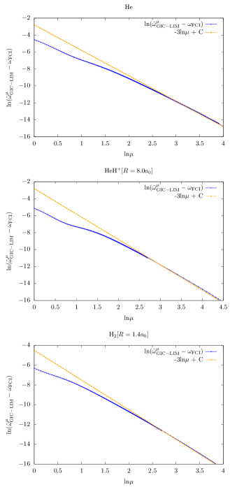
Figure 1: Asymptotic behaviour of the GIC-LIM excitation energy in the large $\mu$ limit for He, the stretched HeH⁺ molecule and H₂ at equilibrium. The excitations considered are: $\{1^{1}{\rm S}\rightarrow 2^{1}{\rm S}\}$ in He, $\{1^{1}\Sigma^{+}\rightarrow 2^{1}\Sigma^{+}\}$ in HeH⁺ and $\{1^{1}\Sigma^{+}_{g}\rightarrow 2^{1}\Sigma^{+}_{g}\}$ in H₂. See text for further details.

II.5 Higher-order extrapolation corrections

As pointed out in Ref. Rebolini et al. (2015b), higher-order energy derivatives can be used in the extrapolation correction in order to further improve on the convergence of ELIM and EGIC-LIM excitation energies towards the FCI results in the large $\mu$ limit. From the Taylor expansion of the WIDFA ensemble energy through third order

$$\tilde{E}^{\mu,{\bf w}}=E^{{\bf w}}+\frac{1}{2}\frac{\tilde{E}^{(-2),{\bf w}}}{\mu^{2}}+\frac{1}{6}\frac{\tilde{E}^{(-3),{\bf w}}}{\mu^{3}}+\mathcal{O}\left(\frac{1}{\mu^{4}}\right),$$ (56)

we obtain

$$\tilde{E}^{\mu,{\bf w}}+\mu\frac{\partial\tilde{E}^{\mu,{\bf w}}}{\partial\mu}+\frac{\mu^{2}}{6}\frac{\partial^{2}\tilde{E}^{\mu,{\bf w}}}{\partial\mu^{2}}=E^{{\bf w}}+\mathcal{O}\left(\frac{1}{\mu^{4}}\right),$$ (57)

thus leading, after linear interpolation, to the following second-order ELIM (ELIM2) excitation energy expression,

$$\tilde{\omega}_{{\rm{ELIM2}},I}^{\mu}=\tilde{\omega}_{{\rm{LIM}},I}^{\mu}+\mu\frac{\partial\tilde{\omega}_{{\rm{LIM}},I}^{\mu}}{\partial\mu}+\frac{\mu^{2}}{6}\frac{\partial^{2}\tilde{\omega}_{{\rm{LIM}},I}^{\mu}}{\partial\mu^{2}},$$ (58)

which is exact through third order in $1/\mu$, like the EGIC-LIM excitation energy. Similarly, from the Taylor expansion of the GIC ensemble energy through fourth order (see the Appendix),

$$\tilde{E}_{\rm{GIC}}^{\mu,{\bf w}}=E^{{\bf w}}+\frac{1}{6}\frac{\tilde{E}_{\rm{GIC}}^{(-3),{\bf w}}}{\mu^{3}}+\frac{1}{24}\frac{\tilde{E}_{\rm{GIC}}^{(-4),{\bf w}}}{\mu^{4}}+\mathcal{O}\left(\frac{1}{\mu^{5}}\right)$$ (59)

it comes

$$\tilde{E}_{\rm{GIC}}^{\mu,{\bf w}}+\frac{2}{3}\mu\frac{\partial\tilde{E}_{\rm{GIC}}^{\mu,{\bf w}}}{\partial\mu}+\frac{1}{12}\mu^{2}\frac{\partial^{2}\tilde{E}_{\rm{GIC}}^{\mu,{\bf w}}}{\partial\mu^{2}}$$

$$=E^{\bf w}+\mathcal{O}\left(\frac{1}{\mu^{5}}\right),$$ (60)

thus leading to the second-order EGIC-LIM (EGIC-LIM2) excitation energy expression,

$$\tilde{\omega}_{{\rm{EGIC-LIM2}},I}^{\mu} = \tilde{\omega}_{{\rm{GIC-LIM}},I}^{\mu}+\frac{2}{3}\mu\frac{\partial\tilde{\omega}_{{\rm{GIC-LIM}},I}^{\mu}}{\partial\mu}$$ (61)

$$+\frac{1}{12}\mu^{2}\frac{\partial^{2}\tilde{\omega}_{{\rm{GIC-LIM}},I}^{\mu}}{\partial\mu^{2}},$$

which is exact through fourth order in $1/\mu$.

III Computational Details

WIDFA (Eq. (29)) and GIC (Eq. (39)) range-separated ensemble energies as well as LIM and GIC-LIM excitation energies (see Eq. (47)), with (Eqs. (51) and (55)) and without extrapolation, have been computed with a development version of the DALTON program package DAL ; Aidas et al. (2015) for a small test set consisting of He, H${}_{2}(R=1.4a_{0},3.7a_{0})$, HeH⁺ and LiH. The extrapolated LIM and GIC-LIM excitation energies (ELIM and EGIC-LIM) have been calculated using finite differences with $\Delta\mu=0.005a_{0}^{-1}$. The long-range-interacting wavefunctions have been calculated using full CI (FCI) level of theory in combination with the spin-independent ground-state short-range local density approximation of Toulouse et al.Toulouse, Savin, and Flad (2004); Toulouse, Colonna, and Savin (2004). The short-range multideterminantal correlation functional of Paziani et al. Paziani et al. (2006) has been used for calculating GIC range-separated ensemble energies and GIC-LIM excitation energies. For all systems but LiH, aug-cc-pVQZ basis sets Dunning Jr (1989); Woon and Dunning Jr (1994) have been used. For LiH, aug-cc-pVTZ basis set with frozen 1s orbital has been used. For calculating the first excitation energy a two-state ensemble is considered in all the cases whereas for the higher excitation energies larger ensembles (three-, four- and five-state ensembles), consisting of singlet states only, are considered. The corresponding two-state ensembles are $\{1^{1}\Sigma^{+},2^{1}\Sigma^{+}\}$ for HeH⁺ and LiH, $\{1^{1}\Sigma^{+}_{g},2^{1}\Sigma^{+}_{g}\}$ for H₂ and $\{1^{1}S,2^{1}S\}$ for He. The larger ensembles have been used for calculating the $\{1^{1}\Sigma^{+}_{g}\rightarrow 3^{1}\Sigma^{+}_{g}\},\{1^{1}\Sigma^{+}_{g}\rightarrow 4^{1}\Sigma^{+}_{g}\}$ and $\{1^{1}\Sigma^{+}_{g}\rightarrow 5^{1}\Sigma^{+}_{g}\}$ excitation energies in H₂ and $\{1^{1}\Sigma^{+}\rightarrow 3^{1}\Sigma^{+}\},\{1^{1}\Sigma^{+}\rightarrow 4^{1}\Sigma^{+}\}$ excitation energies in HeH⁺.

IV Results and discussion

IV.1 Basis set convergence in He

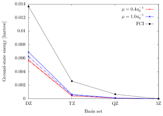
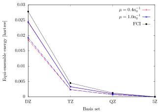
Figure 2: Variation of ground-state energy (top panel) and equi-ensemble energy (bottom panel) with basis set in He. For clarity, the energies relative to aug-cc-pV5Z values are plotted. Basis sets used are aug-cc-pVnZ, where n=2-5. GIC and WIDFA values are represented by solid and dash-dotted lines, respectively. Results for $\mu=0.4a_{0}^{-1}$ and $\mu=1.0a_{0}^{-1}$ are represented by the red and blue colored lines, respectively. For comparison FCI values (black curve) are also plotted.

The performance of LIM and GIC-LIM (with and without extrapolation) has already been discussed for He in Ref.  Alam, Knecht, and Fromager (2016) The purpose of this section is to extend the discussion of Franck et al. Franck et al. (2015) on the basis set convergence of range-separated ground-state energies to ensembles. In Fig. 2, the convergence of WIDFA/GIC ground-state ($w$=0) and equiensemble ($w$=1/2) range-separated energies obtained with aug-cc-pVnZ (n=2,3,4,5) basis sets are shown for the two-state ensemble $\{1^{1}S,2^{1}S\}$ in He with the range-separation parameter set to the typical Fromager, Toulouse, and Jensen (2007); Pastorczak, Gidopoulos, and Pernal (2013) $\mu=0.4a^{-1}_{0}$ and $\mu=1.0a_{0}^{-1}$ values. In comparison to the FCI values, the WIDFA/GIC range-separated energies show faster convergence, especially the ground-state ones. The latter converge at the same rate with both methods whereas, for the equiensemble energies, WIDFA values converge faster than GIC values (which are actually relatively close to the FCI ones). The $\mu$ dependence is not the same for the two energies. Equiensemble energies are less sensitive to the range-separation parameter $\mu$ than the ground-state energy. In fact, the GIC equiensemble energies for the two $\mu$ values overlap. The difference between WIDFA and GIC equiensemble energies as well as their slower convergence with the basis set (when comparison is made with the ground-state energy) are due to the facts that (i) long-range correlation effects are negligible in the ground state but significant in the equiensemble because of the Rydberg character of the excited state and (ii) the GIC energy is less density-dependent than the WIDFA one. Indeed, in the former case, short-range correlation effects only are described by a density functional.

IV.2 LiH

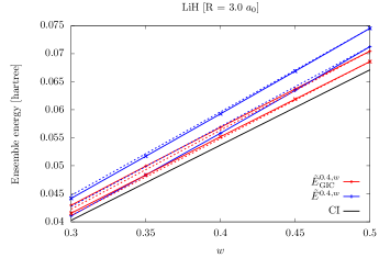
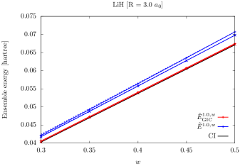
Figure 3: Effect of the extrapolation on the range-separated energy of the two-state $\left\{1^{1}\Sigma^{+},2^{1}\Sigma^{+}\right\}$ ensemble with weight $w$ in LiH $(R=3.0a_{0})$ for $\mu=0.4a_{0}^{-1}$ (top) and $1.0a_{0}^{-1}$ (bottom). Red and blue curves with point type “+” represent the GIC and WIDFA ensemble energies, respectively, whereas the same colored lines with point type “$\times$” represent the corresponding extrapolated values. The dashed lines connecting the two extreme points (i.e. for $w=0.0$ and $w=0.5$) are drawn to show the deviation from linearity.

The effect of extrapolation on the two-state ensemble energy of LiH in the large-$w$ region is shown in Fig. 3 for $\mu=0.4a_{0}^{-1}$ (top panel) and $1.0a_{0}^{-1}$ (bottom panel). It is obvious from these plots that the WIDFA energy and its extrapolation are slightly curved, which is more visible for $\mu=0.4a_{0}^{-1}$, and that they deviate significantly from the CI straight line This is a consequence of using an approximate (weight-independent) ground-state local short-range xc functional, as discussed in Sec. II.2 and Ref. Senjean et al. (2016, 2015) On going from $\mu=0.4a_{0}^{-1}$ to $\mu=1.0a_{0}^{-1}$, although curvature is reduced, the WIDFA energies (with or without extrapolation) still differ from the CI result. In a previous work Alam, Knecht, and Fromager (2016), we have shown that the GIC scheme could almost restore the linearity of the ensemble energy, which is also reflected in Fig. 3. Note that, for $\mu=0.4a_{0}^{-1}$, the extrapolation enlarges the deviation of the WIDFA ensemble energy from the accurate CI result. It only leads to an improvement when the larger $\mu=1.0a_{0}^{-1}$ value is used. On the other hand, GIC energies are always improved after extrapolation. For $\mu=1.0a_{0}^{-1}$, the extrapolated GIC ensemble energy is almost on top of the CI one.

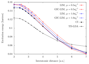
Figure 4: Variation of the first $\Sigma^{+}$ singlet excitation energy with the inter-atomic distance in LiH, for $\mu=0.5a_{0}^{-1}$(red colored lines) and $\mu=1.0a_{0}^{-1}$(blue colored lines). LIM and GIC-LIM values are represented by $\square$ and $\times$, respectively. For comparison, TD-LDA ($\fullmoon$) and CI results ($\blacksquare$) are also plotted.

In Fig. 4, we show the variation of the first $\Sigma^{+}$ singlet excitation energy of LiH with the inter-atomic distance, for $\mu=0.5$ and $1.0a_{0}^{-1}$. The comparison is made with the CI and TD-LDA results. Note that, in contrast to TD-LDA, both LIM and GIC-LIM reproduce relatively well the shape of the CI curve. As expected, GIC-LIM is closer to CI than LIM for the two $\mu$ values. For $\mu=1.0a_{0}^{-1}$, the agreement is actually excellent beyond the equilibrium distance ($R>3a_{0}$). At equilibrium ($R=3a_{0}$), TD-LDA underestimates the excitation energy by 0.0229 a.u. (if comparison is made with the CI result), which was expected since the $2^{1}\Sigma^{+}$ state has a charge-transfer character (from H to Li). On the other hand, GIC-LIM $(\mu=0.5a_{0}^{-1})$ slightly overestimates (by 0.004 a.u.) the excitation energy. For larger bond distances, the failure of TD-LDA might be related to the multiconfigurational character of the $2^{1}\Sigma^{+}$ state. The multideterminantal treatment of the long-range interaction in range-separated eDFT enables a proper description of the excitation energy in the strong correlation regime.

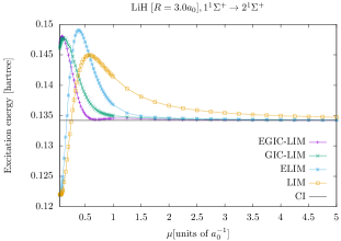
Figure 5: Comparison of EGIC-LIM excitation energy with that obtained from other schemes in LiH. See text for further details.

The performance of the extrapolation scheme is now investigated at the fixed inter-atomic distance $R=3a_{0}$ when varying the range-separation parameter. Results are shown in Fig. 5. One can easily see that EGIC-LIM exhibits the fastest convergence in $\mu$ towards the CI result, as expected. While GIC-LIM and ELIM excitation energies are almost converged at about $\mu=2.0a_{0}^{-1}$, EGIC-LIM reaches the CI result already for the relatively small $\mu=0.75a_{0}^{-1}$ value.

IV.3 HeH⁺

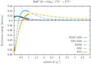
Figure 6: Comparison of EGIC-LIM excitation energy with that obtained from other schemes in the stretched HeH⁺ molecule. See text for further details.

We show in Fig. 6 the convergence of the $1^{1}\Sigma^{+}\rightarrow 2^{1}\Sigma^{+}$ charge-transfer excitation energy with the $\mu$ parameter in the stretched HeH⁺ ($R$=8.0$a_{0}^{-1}$) molecule. As already observed for LiH, EGIC-LIM converges faster (at about $\mu=1.0a_{0}^{-1}$) than the other methods.
We also studied the variation of the $1^{1}\Sigma^{+}\rightarrow n^{1}\Sigma^{+}$ ($n=2,3,4$) excitation energies with the bond length for $\mu=0.4$ and $1.0a_{0}^{-1}$ values. Results are shown in Fig. 7 and comparison is made with FCI and TD-LDA. In contrast to TD-LDA, which significantly underestimates the (charge-transfer) excitation energies, as expected, both LIM and GIC-LIM (with or without extrapolation) are much closer to FCI for all interatomic distances. Interestingly, for $\mu=0.4a_{0}^{-1}$, LIM underestimates the first excitation energy and overestimates the second and third excitation energies whereas, for $\mu=1.0a_{0}^{-1}$, it overestimates all the three excitation energies. After extrapolation, the corresponding ELIM ($\mu=0.4a_{0}^{-1}$) excitation energies increase, which is an improvement only for the first excited state. As expected, GIC-LIM performs better than LIM and ELIM. It slightly overestimates all excitation energies for both $\mu$ values. The impact of the extrapolation correction on the curves is hardly visible. Note that, for $\mu$=$1.0a_{0}^{-1}$, EGIC-LIM and FCI curves are almost on top of each other. Finally, even for the relatively small range-separation parameter value $\mu=0.4a_{0}^{-1}$, the avoided crossing between the second and third excited states at about $R=4.0a_{0}$ is well reproduced by GIC-LIM (with or without extrapolation).

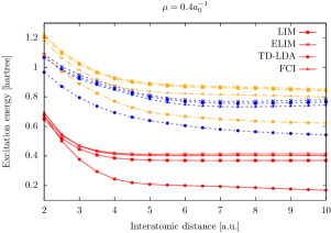
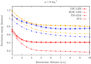
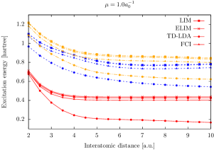
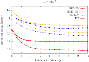
Figure 7: Variation of first (red curves; $1^{1}\Sigma^{+}\rightarrow 2^{1}\Sigma^{+}$), second (blue curves; $1^{1}\Sigma^{+}\rightarrow 3^{1}\Sigma^{+}$) and third (orange curves; $1^{1}\Sigma^{+}\rightarrow 4^{1}\Sigma^{+}$) excitation energies with the interatomic distance in HeH⁺. The following markers are used to distinguish results obtained from different methods – LIM (or GIC-LIM): $\blacksquare$, ELIM (or EGIC-LIM): $\times$, TD-LDA: $\newmoon$, and FCI: $\blacktriangle$.

IV.4 Convergence in $\mu$ of higher-order extrapolation schemes

The variation with $\mu$ of the excitation energies obtained for He and HeH⁺ with second-order extrapolation schemes (see Eqs. (58) and (61)) are shown in Fig. 8. As expected, ELIM2 and EGIC-LIM decay similarly in the large $\mu$ limit. Nevertheless, the GIC still ensures a faster convergence in $\mu$ towards the FCI result. Regarding the GIC-LIM results, we observe a systematic improvement on the excitation energies when adding higher-order extrapolation corrections in the typical range $0.4\leq\mu\leq 1.0$. Note that EGIC-LIM2 reaches the FCI result for $\mu\sim 0.9a_{0}^{-1}$, which is remarkable. This clearly demonstrates that GIC ensemble energies can give very accurate excitation energies after extrapolation for relatively small range-separation parameter values. Since EGIC-LIM is already accurate for typical $\mu$ values, second-order extrapolation corrections will not be considered in the rest of the discussion.

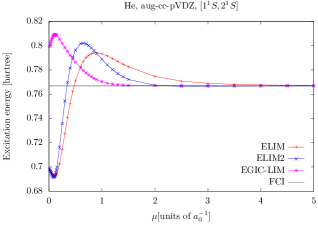
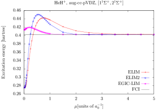
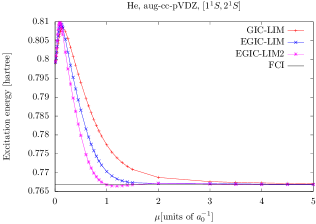
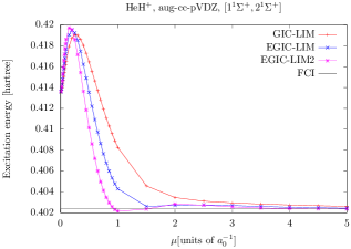
Figure 8: Variation of excitation energies (top panels: ELIM, ELIM2 and EGIC-LIM, bottom panels: GIC-LIM, EGIC-LIM and EGIC-LIM2) with $\mu$ for He (left panels) and HeH⁺ (right panels).

IV.5 H₂

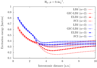
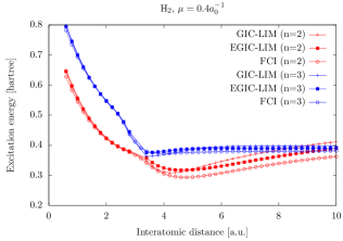
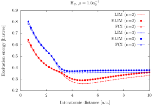
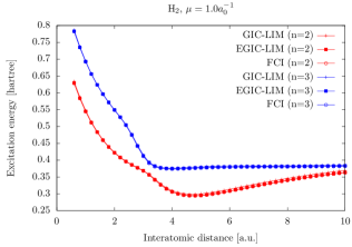
Figure 9: Variation of the $1^{1}\Sigma_{g}^{+}\rightarrow n^{1}\Sigma_{g}^{+}$ excitation energy in H₂ for $n$=2 and 3 with the interatomic distance. Results are shown for $\mu=0.4a_{0}^{-1}$ (top panels) and $\mu=1.0a_{0}^{-1}$ (bottom panels).

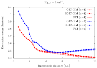
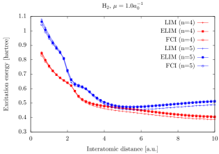
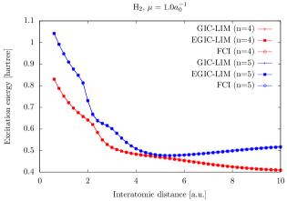
Figure 10: Variation of the $1^{1}\Sigma_{g}^{+}\rightarrow n^{1}\Sigma_{g}^{+}$ excitation energy in H₂ for $n$=4 and 5 with the interatomic distance. Results are shown for $\mu=0.4a_{0}^{-1}$ (top panels) and $\mu=1.0a_{0}^{-1}$ (bottom panels).

Excitation energies have been computed for the first and second (see Fig. 9) as well as third and fourth (see Fig. 10) ${}^{1}\Sigma_{g}^{+}$ excited states of H₂ along the bond breaking coordinate with $\mu=0.4$ and $1.0a_{0}^{-1}$. Comparison is made with FCI. Recently, the first and second excitation energies obtained with the LIM and ELIM methods have been reported and discussed in detail by Senjean et al. in Ref. Senjean et al. (2016) Note that, around the equilibrium distance ($R=1.4a_{0}$), they are both relatively close to the FCI value, especially when $\mu=1.0a_{0}^{-1}$. Substantial differences appear when stretching the bond. LIM underestimates the four excitation energies when $R>3a_{0}$, in particular for $\mu=0.4a_{0}^{-1}$. The extrapolation improves on the results significantly but, for $\mu=0.4a_{0}^{-1}$, the ELIM excitation energies are still too low. The overall performance of GIC-LIM, when compared to LIM and ELIM, is far better. Still, for $\mu=0.4a_{0}^{-1}$, GIC-LIM overestimates the excitation energies in the large-$R$ region. The extrapolation slightly improves on the results. With the larger $\mu=1.0a_{0}^{-1}$ value, GIC-LIM and FCI potential curves are almost on top of each other. Small differences are visible at large distances where the extrapolation correction actually brings some improvement.
Let us now focus on the avoided crossing between the first and second excited states at $\sim 3.5a_{0}$. Beyond this distance the first excited state corresponds to a double excitation. This is the reason why, in contrast to any eDFT-based method, standard (adiabatic) TD-LDA does not exhibit any avoided crossing Fromager, Knecht, and Aa. Jensen (2013). We note that, for $\mu=0.4a_{0}^{-1}$, GIC-LIM improves on the individual excitation energies when compared to LIM but the two states are then too close in energy. The extrapolation slightly improves on GIC-LIM in this respect while making, when applied to LIM, the two states even closer in energy as already shown in Ref. Senjean et al. (2016) For $\mu=1.0a_{0}^{-1}$, the extrapolation brings larger improvement on the LIM values than the GIC-LIM ones. Regarding the third and fourth excitation energies, two avoided crossings are found at $\sim 2.4a_{0}$ and $\sim 5.0a_{0}$. Note that at the second avoided crossing the two FCI curves are closer to each other than at the first avoided crossing. Noticeably, for $\mu=0.4a_{0}^{-1}$, this behavior is reproduced by GIC-LIM but not by LIM. At the second avoided crossing, the two GIC-LIM curves are closer to each other than the FCI curves. In contrast to EGIC-LIM results, the two ELIM curves cross at $R\sim 2.4a_{0}$. For $\mu=1.0a_{0}^{-1}$, both ELIM and EGIC-LIM are able to reproduce the two avoided crossings. Note that, for the second avoided crossing, EGIC-LIM is substantially improved by increasing $\mu$ from 0.4 to $1.0a_{0}^{-1}$.

V Perspective: extracting individual state energies from range-separated ensemble energies

Having access to state energies rather than ensemble energies or excitation energies is important for modeling properties like equilibrium structures in the excited states. While the extraction of individual energies from the ensemble energy is trivial in pure wavefunction theory Helgaker, Jørgensen, and Olsen (2004), it is still unclear how this can be achieved rigorously and efficiently (in terms of computational cost) in the context of eDFT. As readily seen from Eq. (46), the individual state energy $E_{I}$ can be obtained (in principle exactly) from two equiensemble energies,

$$E_{I}=\dfrac{1}{\mathrm{g}_{I}}\left(M_{I}E^{1/M_{I}}_{I}-M_{I-1}E^{1/M_{I-1}}_{I-1}\right),$$ (62)

the two equiensembles containing up to and including the multiplets with energies $E_{I}$ and $E_{I-1}$, respectively. The disadvantage of such a formulation is that it is not straightforward to calculate the energy of any state belonging to the ensemble of interest. Following the idea of Levy and Zahariev Levy and Zahariev (2014), we propose to rewrite the exact range-separated density-functional ensemble energy in Eq. (24) as a weighted sum of individual long-range interacting energies. This can be achieved by introducing a density-functional shift

$$C^{\rm{\mu,{\bf w}}}[n]=\dfrac{E^{\rm{sr,\mu,{\bf w}}}_{{\rm{Hxc}}}[n]-\int d{\bf r}~{}\dfrac{\delta E_{\rm Hxc}^{\rm{sr,\mu,{\bf w}}}[n]}{\delta n({\bf r})}n({\bf r})}{\int d{\bf r}~{}n({\bf r})}$$ (63)

to the ensemble short-range potential in Eq. (28), thus leading to the ”shifted” eigenvalue equation

$$\Bigg{(} \hat{T}+\hat{W}_{\rm{ee}}^{\rm{lr,\mu}}+\hat{V}_{\rm{ne}}+\int d{\bf r}\Bigg{[}\frac{\delta E_{\rm{Hxc}}^{\rm{sr,\mu,{\bf w}}}[n_{\hat{\Gamma}^{\rm{\mu,{\bf w}}}}]}{\delta n({\bf r})}$$ (64)

$$+C^{\rm{\mu,{\bf w}}}[n_{\hat{\Gamma}^{\rm{\mu,{\bf w}}}}]\Bigg{]}\hat{n}({\bf r})\Bigg{)}|\Psi_{k}^{\rm{\mu,{\bf w}}}\rangle=\overline{\mathcal{E}}_{k}^{\rm{\mu,{\bf w}}}|\Psi_{k}^{\rm{\mu,{\bf w}}}\rangle,$$

where

$$\overline{\mathcal{E}}_{k}^{\rm{\mu,{\bf w}}}=\mathcal{E}^{\rm{\mu,{\bf w}}}_{k}+C^{\rm{\mu,{\bf w}}}[n_{\hat{\Gamma}^{\rm{\mu,{\bf w}}}}]\int d{\bf r}\;n_{\Psi_{k}^{\rm{\mu,{\bf w}}}}({\bf r}),$$ (65)

so that, according to Eqs. (24), (28) and (63), the exact range-separated ensemble energy can be rewritten as follows,

$$E^{\rm{\bf w}} = \sum\limits_{k=0}^{M-1}w_{k}{\mathcal{E}}^{\rm{\mu,{\bf w}}}_{k}+C^{\rm{\mu,{\bf w}}}[n_{\hat{\Gamma}^{\rm{\mu,{\bf w}}}}]\int d{\bf r}\;n_{\hat{\Gamma}^{\rm{\mu,{\bf w}}}}({\bf r})$$ (66)

$$= \sum\limits_{k=0}^{M-1}w_{k}\overline{\mathcal{E}}^{\rm{\mu,{\bf w}}}_{k}.$$

It then becomes natural to interpret each (weight- and $\mu$-dependent) individual shifted energy $\overline{\mathcal{E}}^{\rm{\mu,{\bf w}}}_{k}$ as an approximation to the exact individual state energy $E_{k}$ which is actually recovered for any ensemble weight when $\mu\rightarrow+\infty$. If we now expand the short-range Hxc energy and potential around each individual state density through first order in $\delta n^{\rm{\mu,{\bf w}}}_{k}=n_{\hat{\Gamma}^{\rm{\mu,{\bf w}}}}-n_{\Psi^{\rm{\mu,{\bf w}}}_{k}}$ it comes

$$\overline{\mathcal{E}}_{k}^{\rm{\mu,{\bf w}}} = \left\langle\Psi_{k}^{\rm{\mu,{\bf w}}}\middle|\hat{T}+\hat{W}_{\rm{ee}}^{\rm{lr,\mu}}+\hat{V}_{\rm{ne}}\middle|\Psi_{k}^{\rm{\mu,{\bf w}}}\right\rangle+E_{\rm{Hxc}}^{\rm{sr,\mu,{\bf w}}}[n_{\hat{\Gamma}^{\rm{\mu,{\bf w}}}}]$$ (67)

$$-\int d{\bf r}\frac{\delta E_{\rm{Hxc}}^{\rm{sr,\mu,{\bf w}}}[n_{\hat{\Gamma}^{\rm{\mu,{\bf w}}}}]}{\delta n({\bf r})}\delta n^{\rm{\mu,{\bf w}}}_{k}({\bf r})$$

$$= \left\langle\Psi_{k}^{\rm{\mu,{\bf w}}}\middle|\hat{T}+\hat{W}_{\rm{ee}}^{\rm{lr,\mu}}+\hat{V}_{\rm{ne}}\middle|\Psi_{k}^{\rm{\mu,{\bf w}}}\right\rangle+E_{\rm{Hxc}}^{\rm{sr,\mu,{\bf w}}}[n_{\Psi_{k}^{\rm{\mu,{\bf w}}}}]$$

$$+\mathcal{O}\left[\left(\delta n^{\rm{\mu,{\bf w}}}_{k}\right)^{2}\right],$$

where we used the fact that both ensemble and individual densities integrate to the number of electrons, according to the normalization condition in Eq. (1). Interestingly, when the WIDFA approximation is used, the individual state energy expression proposed by Pastorczak et al. Pastorczak, Gidopoulos, and Pernal (2013) for computing approximate excitation energies is recovered from Eq. (67) through first order in $\delta n^{\rm{\mu,{\bf w}}}_{k}$. In the latter case, the use of individual densities automatically removes ghost interaction errors Pastorczak and Pernal (2016). The implementation and calibration of the first line of Eq. (67) within WIDFA is currently in progress and will be presented in a separate paper.

VI Conclusion

The extrapolation technique introduced by Savin Savin (2014) in the context of ground-state range-separated DFT has been extended to ghost-interaction-corrected (GIC) ensemble energies of ground and excited states. While the standard extrapolation correction relies on a Taylor expansion of the range-separated energy that decays as $\mu^{-2}$ in the $\mu\rightarrow+\infty$ limit, where $\mu$ is the range-separation parameter, the GIC ensemble energy was shown to decay more rapidly as $\mu^{-3}$, thus requiring a different extrapolation correction. The approach has been combined with a linear interpolation (between equiensembles) method in order to compute excitation energies. Promising results have been obtained for singlet excitations (including charge transfer and double excitations) on a small test set consisting of He, H₂, HeH⁺ and LiH. In particular, avoided crossings could be described accurately in H₂ by setting the range-separation parameter to $\mu=1.0a_{0}^{-1}$, which is a typical value in range-separated eDFT calculations Pastorczak, Gidopoulos, and Pernal (2013); Pastorczak and Pernal (2016). Interestingly, convergence towards the pure wavefunction theory result ($\mu\rightarrow+\infty$ limit) is essentially reached for $\mu=1.0a_{0}^{-1}$ thanks to both ghost-interaction and extrapolation corrections. As expected, the results can be further improved for smaller $\mu$ values with higher-order extrapolation corrections. The method is currently applied to the modeling of conical intersections, which is still challenging for TD-DFT. Finally, the extraction of individual state energies from range-separated ensemble energies has been discussed as a perspective. Approximate energies have been constructed by introducing an ensemble-density-functional shift in the exchange-correlation potential. We could show that, by expanding these energies around the individual densities, the ghost-interaction-free expressions of Pastorczak et al. Pastorczak, Gidopoulos, and Pernal (2013) are recovered through first order. The implementation and development of this approach, for the calculation of excited-state molecular gradients, for example, is left for future work.

VII Acknowledgements

The authors acknowledge financial support from the LABEX ‘Chemistry of complex systems’ and the ANR [MCFUNEX project, Grant No. ANR-14-CE06- 0014-01].

Appendix A Taylor expansion of the range-separated GIC ensemble energy for large $\mu$ values.

Let $\eta=1/\mu$ so that the range-separated GIC ensemble energy can be Taylor expanded as follows for large $\mu$ values,

$$\tilde{E}_{\rm{GIC}}^{1/\eta,{\bf w}}= E^{\bf w}+\tilde{E}_{\rm{GIC}}^{(-1),{\bf w}}\eta+\frac{1}{2}\tilde{E}_{\rm{GIC}}^{(-2),{\bf w}}\eta^{2}+\frac{1}{6}\tilde{E}_{\rm{GIC}}^{(-3),{\bf w}}\eta^{3}$$ (68)

$$+\mathcal{O}(\eta^{4}),$$

where

$$\begin{array}[]{l}\begin{split}\tilde{E}_{\rm{GIC}}^{(-1),{\bf w}}&=\left.\frac{\partial\tilde{E}_{\rm{GIC}}^{\rm{1/\eta},{\bf w}}}{\partial\eta}\right|_{\eta=0},\\ \tilde{E}_{\rm{GIC}}^{(-2),{\bf w}}&=\left.\frac{\partial^{2}\tilde{E}_{\rm{GIC}}^{\rm{1/\eta},{\bf w}}}{\partial\eta^{2}}\right|_{\eta=0}.\end{split}\end{array}$$ (70)

We will show that these two derivatives vanish and hence the first $\eta$-dependence of $\tilde{E}_{\rm{GIC}}^{1/\eta,{\bf w}}$ appears at third order. According to Eq. (39), we have (using real algebra)

$$\begin{array}[]{l}\begin{split}\frac{\partial\tilde{E}_{\rm{GIC}}^{1/\eta,{\bf w}}}{\partial\eta}=&\sum\limits_{k=0}^{M-1}2w_{k}\left.\left.\left\langle\frac{\partial\tilde{\Psi}_{k}^{1/\eta,{\bf w}}}{\partial\eta}\right|\hat{H}\right|\tilde{\Psi}_{k}^{1/\eta,{\bf w}}\right\rangle\\ &+\frac{\partial E_{\rm{c,md}}^{{\rm{sr}},1/\eta}[n_{\hat{\gamma}^{1/\eta,{\bf w}}}]}{\partial\eta},\\ \frac{\partial^{2}\tilde{E}_{\rm{GIC}}^{1/\eta,{\bf w}}}{\partial\eta^{2}}=&\sum\limits_{k=0}^{M-1}2w_{k}\left\{\left.\left.\left\langle\frac{\partial^{2}\tilde{\Psi}_{k}^{1/\eta,{\bf w}}}{\partial\eta^{2}}\right|\hat{H}\right|\tilde{\Psi}_{k}^{1/\eta,{\bf w}}\right\rangle\right.\\ &+\left.\left.\left.\left\langle\frac{\partial\tilde{\Psi}_{k}^{1/\eta,{\bf w}}}{\partial\eta}\right|\hat{H}\right|\frac{\partial\tilde{\Psi}_{k}^{1/\eta,{\bf w}}}{\partial\eta}\right\rangle\right\}\\ &+\frac{\partial^{2}E_{\rm{c,md}}^{{\rm{sr}},1/\eta}[n_{\hat{\gamma}^{1/\eta,{\bf w}}}]}{\partial\eta^{2}}.\end{split}\end{array}$$ (72)

Since  Toulouse, Gori-Giorgi, and Savin (2005)

$$\begin{array}[]{l}E_{\rm{c,md}}^{\rm{sr,1/\eta}}[n]=E_{\rm{c,md}}^{(-3)}[n]\;\eta^{3}+\mathcal{O}(\eta^{4}),\end{array}$$ (74)

the last term on the right-hand side of both equalities in Eq. (72) vanishes when $\eta=0$. Furthermore, according to Eq. (30),

$$\begin{array}[]{l}\begin{split}\left.\left.\left.\left\langle\frac{\partial\tilde{\Psi}_{k}^{1/\eta,{\bf w}}}{\partial\eta}\right|\hat{H}\right|\tilde{\Psi}_{k}^{1/\eta,{\bf w}}\right\rangle\right|_{\eta=0}=E_{k}\left.\left\langle\left.\frac{\partial\tilde{\Psi}_{k}^{1/\eta,{\bf w}}}{\partial\eta}\right|{\Psi}_{k}\right\rangle\right|_{\eta=0}\end{split}\end{array}$$ (76)

and

$$\begin{array}[]{l}\begin{split}\left.\left.\left.\left\langle\frac{\partial^{2}\tilde{\Psi}_{k}^{1/\eta,{\bf w}}}{\partial\eta^{2}}\right|\hat{H}\right|\tilde{\Psi}_{k}^{1/\eta,{\bf w}}\right\rangle\right|_{\eta=0}=E_{k}\left.\left\langle\left.\frac{\partial^{2}\tilde{\Psi}_{k}^{1/\eta,{\bf w}}}{\partial\eta^{2}}\right|{\Psi}_{k}\right\rangle\right|_{\eta=0}.\end{split}\end{array}$$ (78)

Since the long-range-interacting wavefunction is normalized for any value of the range-separation parameter,

$$\begin{array}[]{l}\begin{split}&\forall\eta\hskip 5.69046pt\left.\left\langle\tilde{\Psi}_{k}^{1/\eta,{\bf w}}\right|\tilde{\Psi}_{k}^{1/\eta,{\bf w}}\right\rangle=1,\end{split}\end{array}$$ (80)

it comes

$$\begin{array}[]{l}\begin{split}\left.\left.\left\langle\frac{\partial\tilde{\Psi}_{k}^{1/\eta,{\bf w}}}{\partial\eta}\right|{\Psi}_{k}\right\rangle\right|_{\eta=0}=0\end{split}\end{array}$$ (82)

and

$$\begin{array}[]{l}\begin{split}\left.\left.\left\langle\frac{\partial^{2}\tilde{\Psi}_{k}^{1/\eta,{\bf w}}}{\partial\eta^{2}}\right|{\Psi}_{k}\right\rangle\right|_{\eta=0}=-\left.\left\langle\left.\frac{\partial\tilde{\Psi}_{k}^{1/\eta,{\bf w}}}{\partial\eta}\right|\frac{\partial\tilde{\Psi}_{k}^{1/\eta,{\bf w}}}{\partial\eta}\right\rangle\right|_{\eta=0}.\end{split}\end{array}$$ (84)

Combining Eqs. (70), (72), (76), (78), (82) and (84) leads to

$$\begin{array}[]{l}\tilde{E}_{\rm{GIC}}^{(-1),{\bf w}}=0\end{array}$$ (86)

and

$$\tilde{E}_{\rm{GIC}}^{(-2),{\bf w}}=\sum\limits_{k=0}^{M-1}2w_{k}\left.\left.\left\langle\left.\frac{\partial\tilde{\Psi}_{k}^{1/\eta,{\bf w}}}{\partial\eta}\right|\hat{H}-E_{k}\right|\frac{\partial\tilde{\Psi}_{k}^{1/\eta,{\bf w}}}{\partial\eta}\right\rangle\right|_{\eta=0}.$$ (87)

By applying first-order perturbation theory to Eq. (30) we obtain

$${\dfrac{\partial\left|\tilde{\Psi}_{k}^{1/\eta,{\bf w}}\right\rangle}{\partial\eta}=\sum^{+\infty}_{l\neq k}\dfrac{\left\langle\tilde{\Psi}_{l}^{1/\eta,{\bf w}}|\hat{\mathcal{W}}^{1/\eta}|\tilde{\Psi}_{k}^{1/\eta,{\bf w}}\right\rangle}{\tilde{\mathcal{E}}_{k}^{1/\eta,{\bf w}}-\tilde{\mathcal{E}}_{l}^{1/\eta,{\bf w}}}\left|\tilde{\Psi}_{l}^{1/\eta,{\bf w}}\right\rangle,}$$ (88)

where the perturbation operator reads

$$\hat{\mathcal{W}}^{1/\eta}=\frac{\partial\hat{W}_{\rm{ee}}^{\rm{lr,1/\eta}}}{\partial\eta}+\int d{\bf r}\frac{\partial}{\partial\eta}\frac{\delta E_{\rm{Hxc}}^{\rm{sr,1/\eta}}[n_{\hat{\gamma}^{1/\eta,{\bf w}}}]}{\delta n({\bf r})}\hat{n}({\bf r}).$$ (89)

Note that the second term on the right-hand side of Eq. (89) vanishes when $\eta=0$ since Toulouse, Colonna, and Savin (2004); Gori-Giorgi and Savin (2006)

$$\begin{array}[]{l}E_{\rm{Hxc}}^{\rm{sr},1/\eta}[n]=E_{\rm{Hxc}}^{(-2)}[n]\,\eta^{2}+\mathcal{O}(\eta^{3}),\end{array}$$ (91)

thus leading to

$$\begin{array}[]{l}\begin{split}\displaystyle&\left.\left.\left\langle\left.\frac{\partial\tilde{\Psi}_{k}^{1/\eta,{\bf w}}}{\partial\eta}\right|\hat{H}-E_{k}\right|\frac{\partial\tilde{\Psi}_{k}^{1/\eta,{\bf w}}}{\partial\eta}\right\rangle\right|_{\eta=0}\\ &=-\sum^{+\infty}\limits_{l\neq k}\frac{1}{E_{k}-E_{l}}\left.\left.\left.\left|\left\langle\Psi_{l}\left|\frac{\partial\hat{W}_{\rm{ee}}^{\rm{lr,1/\eta}}}{\partial\eta}\right.\right|\Psi_{k}\right.\right\rangle\right|^{2}\right|_{\eta=0}.\end{split}\end{array}$$ (93)

Finally, using Senjean et al. (2016)

$$\begin{array}[]{l}\displaystyle\frac{\partial\hat{W}^{\rm{lr,1/\eta}}_{\rm{ee}}}{\partial\eta}=-8\sqrt{\pi}\int^{+\infty}_{0}d{{{r}}_{12}}\frac{r_{12}^{2}}{\eta^{2}}e^{-\frac{r_{12}^{2}}{\eta^{2}}}\hat{f}({{r}}_{12}),\end{array}$$ (95)

where $r_{12}=|{\bf r}_{1}-{\bf r}_{2}|$ is the interelectronic distance and $\hat{f}({{r}}_{12})$ is the intracule density operator, we obtain

$$\left.\left.\left\langle\Psi_{l}\left|\frac{\partial\hat{W}_{\rm{ee}}^{\rm{lr,1/\eta}}}{\partial\eta}\right.\right|\Psi_{k}\right.\right\rangle=-8\sqrt{\pi} \int^{+\infty}_{0}d{{{r}}_{12}}\frac{r_{12}^{2}}{\eta^{2}}\text{exp}\left({-\frac{r_{12}^{2}}{\eta^{2}}}\right)$$ (96)

$$\times\left\langle\Psi_{l}\left|\hat{f}({{r}}_{12})\right|\Psi_{k}\right\rangle.$$

Since $\frac{r_{12}^{2}}{\eta^{2}}\text{exp}\left({-\frac{r_{12}^{2}}{\eta^{2}}}\right)\rightarrow 0$ when $\eta\rightarrow 0$ for all values of $r_{12}$, we conclude from Eqs. (87) and (93) that

$$\begin{array}[]{l}\tilde{E}_{\rm{GIC}}^{(-2),{\bf w}}=0,\end{array}$$ (98)

so that Eq. (68) can be simplified as follows,

$$\begin{array}[]{l}\tilde{E}_{\rm{GIC}}^{1/\eta,{\bf w}}=E^{\bf w}+\dfrac{1}{6}\tilde{E}_{\rm{GIC}}^{(-3),{\bf w}}\eta^{3}+\mathcal{O}(\eta^{4}),\end{array}$$ (100)

thus leading to the expansion in Eq. (52).

References

- Hohenberg and Kohn (1964) P. Hohenberg and W. Kohn, Phys. Rev. 136, B864 (1964).
- Kohn and Sham (1965) W. Kohn and L. Sham, Phys. Rev. 140, A1133 (1965).
- Runge and Gross (1984) E. Runge and E. K. U. Gross, Phys. Rev. Lett. 52, 997 (1984).
- Casida and Huix-Rotllant (2012) M. Casida and M. Huix-Rotllant, Annu. Rev. Phys. Chem. 63, 287 (2012).
- Casida (1995) M. Casida, in Recent Advances in Density Functional Methods, edited by D. P. Chong (World Scientific, Singapore, 1995).
- Marques and Gross (2004) M. Marques and E. Gross, Annu. Rev. Phys. Chem. 55, 427 (2004).
- Gunnarsson and Lundqvist (1976) O. Gunnarsson and B. I. Lundqvist, Phys. Rev. B 13, 4274 (1976).
- Dederichs et al. (1984) P. H. Dederichs, S. Blügel, R. Zeller, and H. Akai, Phys. Rev. Lett. 53, 2512 (1984).
- Ziegler, Rauk, and Baerends (1977) T. Ziegler, A. Rauk, and E. J. Baerends, Theor. Chim. Acta 43, 261 (1977).
- von Barth (1979) U. von Barth, Phys. Rev. A 20, 1693 (1979).
- Theophilou (1979) A. K. Theophilou, J. Phys. C (Solid State Phys.) 12, 5419 (1979).
- Gross, Oliveira, and Kohn (1988a) E. K. U. Gross, L. N. Oliveira, and W. Kohn, Phys. Rev. A 37, 2805 (1988a).
- Gross, Oliveira, and Kohn (1988b) E. K. U. Gross, L. N. Oliveira, and W. Kohn, Phys. Rev. A 37, 2809 (1988b).
- Gross, Oliveira, and Kohn (1988c) E. K. U. Gross, L. N. Oliveira, and W. Kohn, Phys. Rev. A 37, 2821 (1988c).
- Nagy (1996) Á. Nagy, J. Phys. B: At. Mol. Opt. Phys. 29, 389 (1996).
- Tasnádi and Nagy (2003) F. Tasnádi and Á. Nagy, Journal of Physics B: Atomic, Molecular and Optical Physics 36, 4073 (2003).
- Gritsenko et al. (2000) O. Gritsenko, S. Van Gisbergen, A. Gorling, and E. Baerends, J. Chem. Phys. 113, 8478 (2000).
- Casida et al. (1998) M. E. Casida, C. Jamorski, K. C. Casida, and D. R. Salahub, J. Chem. Phys. 108, 4439 (1998).
- Dreuw, Weisman, and Head-Gordon (2003) A. Dreuw, J. L. Weisman, and M. Head-Gordon, J. Chem. Phys. 119, 2943 (2003).
- Maitra et al. (2004) N. T. Maitra, F. Zhang, R. J. Cave, and K. Burke, J. Chem. Phys. 120, 5932 (2004).
- Savin (1988) A. Savin, Int. J. Quantum Chem. 34, 59 (1988).
- Stoll and Savin (1985) H. Stoll and A. Savin, in Density Functional Methods in Physics, edited by R. M. Dreizler and J. da Providencia (Plenum, New York, 1985).
- Savin (1996) A. Savin, Recent Developments and Applications of Modern Density Functional Theory (Elsevier, Amsterdam, 1996) p. 327.
- Huix-Rotllant et al. (2011) M. Huix-Rotllant, A. Ipatov, A. Rubio, and M. E. Casida, Chem. Phys. 391, 120 (2011).
- Filatov, Huix-Rotllant, and Burghardt (2015) M. Filatov, M. Huix-Rotllant, and I. Burghardt, J. Chem. Phys. 142, 184104 (2015).
- Krykunov and Ziegler (2013) M. Krykunov and T. Ziegler, Journal of Chemical Theory and Computation 9, 2761 (2013), pMID: 26583867, http://dx.doi.org/10.1021/ct300891k .
- Ziegler et al. (2009) T. Ziegler, M. Seth, M. Krykunov, J. Autschbach, and F. Wang, The Journal of Chemical Physics 130, 154102 (2009), http://dx.doi.org/10.1063/1.3114988 .
- Glushkov and Levy (2016) V. Glushkov and M. Levy, Computation 4 (2016), 10.3390/computation4030028.
- Ayers and Levy (2009) P. W. Ayers and M. Levy, Phys. Rev. A 80, 012508 (2009).
- Yang et al. (2017) Z.-h. Yang, A. Pribram-Jones, K. Burke, and C. A. Ullrich, Phys. Rev. Lett. 119, 033003 (2017).
- Pastorczak, Gidopoulos, and Pernal (2013) E. Pastorczak, N. I. Gidopoulos, and K. Pernal, Phys. Rev. A 87, 062501 (2013).
- Franck and Fromager (2014) O. Franck and E. Fromager, Mol. Phys. 112, 1684 (2014).
- Deur, Mazouin, and Fromager (2017) K. Deur, L. Mazouin, and E. Fromager, Phys. Rev. B 95, 035120 (2017).
- Theophilou (1987) A. K. Theophilou, The single particle density in physics and chemistry, edited by N. H. March and B. M. Deb (Academic Press, 1987) pp. 210–212.
- Kohn (1986) W. Kohn, Phys. Rev. A 34, 737 (1986).
- Nagy (1998) A. Nagy, Int. J. Quantum Chem. 69, 247 (1998).
- Nagy (2001) A. Nagy, J. Phys. B: At. Mol. Opt. Phys. 34, 2363 (2001).
- Yang et al. (2014) Z.-h. Yang, J. R. Trail, A. Pribram-Jones, K. Burke, R. J. Needs, and C. A. Ullrich, Phys. Rev. A 90, 042501 (2014).
- Pribram-Jones et al. (2014) A. Pribram-Jones, Z. hui Yang, J. R.Trail, K. Burke, R. J.Needs, and C. A.Ullrich, J. Chem. Phys. 140, 18A541 (2014).
- Senjean et al. (2015) B. Senjean, S. Knecht, H. J. A. Jensen, and E. Fromager, Phys. Rev. A 92, 012518 (2015).
- Gidopoulos, Papaconstantinou, and Gross (2002) N. Gidopoulos, P. Papaconstantinou, and E. Gross, Phys. Rev. Lett. 88, 033003 (2002).
- Pastorczak and Pernal (2014) E. Pastorczak and K. Pernal, J. Chem. Phys. 140, 18A514 (2014).
- Pastorczak and Pernal (2016) E. Pastorczak and K. Pernal, Int. J. Quantum Chem. (2016), http://dx.doi.org/10.1002/qua.25107.
- Alam, Knecht, and Fromager (2016) M. M. Alam, S. Knecht, and E. Fromager, Physical Review A 94, 012511 (2016).
- Fromager, Toulouse, and Jensen (2007) E. Fromager, J. Toulouse, and H. J. A. Jensen, J. Chem. Phys. 126, 074111 (2007).
- Gerber and Ángyán (2005) I. C. Gerber and J. G. Ángyán, Chem. Phys. Lett. 415, 100 (2005).
- Franck et al. (2015) O. Franck, B. Mussard, E. Luppi, and J. Toulouse, J. Chem. Phys. 142, 074107 (2015).
- Senjean et al. (2016) B. Senjean, E. D. Hedegård, M. M. Alam, S. Knecht, and E. Fromager, Mol. Phys. 114, 968 (2016).
- Savin (2014) A. Savin, J. Chem. Phys. 140, 18A509 (2014).
- Rebolini et al. (2015a) E. Rebolini, J. Toulouse, A. M. Teale, T. Helgaker, and A. Savin, Phys. Rev. A 91, 032519 (2015a).
- Toulouse, Colonna, and Savin (2004) J. Toulouse, F. Colonna, and A. Savin, Phys. Rev. A 70, 062505 (2004).
- Goll, Werner, and Stoll (2005) E. Goll, H. J. Werner, and H. Stoll, Phys. Chem. Chem. Phys. 7, 3917 (2005).
- Toulouse, Gori-Giorgi, and Savin (2005) J. Toulouse, P. Gori-Giorgi, and A. Savin, Theor. Chem. Acc. 114, 305 (2005).
- Paziani et al. (2006) S. Paziani, S. Moroni, P. Gori-Giorgi, and G. B. Bachelet, Phys. Rev. B 73, 155111 (2006).
- Rebolini et al. (2015b) E. Rebolini, J. Toulouse, A. M. Teale, T. Helgaker, and A. Savin, Phys. Rev. A 91, 032519 (2015b).
- (56) “Dalton, a molecular electronic structure program, release dalton2015 (2015), see http://daltonprogram.org/,” .
- Aidas et al. (2015) K. Aidas, C. Angeli, K. L. Bak, V. Bakken, R. Bast, L. Boman, O. Christiansen, R. Cimiraglia, S. Coriani, P. Dahle, E. K. Dalskov, U. Ekström, T. Enevoldsen, J. J. Eriksen, P. Ettenhuber, B. Fernández, L. Ferrighi, H. Fliegl, L. Frediani, K. Hald, A. Halkier, C. Hättig, H. Heiberg, T. Helgaker, A. C. Hennum, H. Hettema, E. Hjertenæs, S. Høst, I.-M. Høyvik, M. F. Iozzi, B. Jansík, H. J. Aa. Jensen, D. Jonsson, P. Jørgensen, J. Kauczor, S. Kirpekar, T. Kjærgaard, W. Klopper, S. Knecht, R. Kobayashi, H. Koch, J. Kongsted, A. Krapp, K. Kristensen, A. Ligabue, O. B. Lutnæs, J. I. Melo, K. V. Mikkelsen, R. H. Myhre, C. Neiss, C. B. Nielsen, P. Norman, J. Olsen, J. M. H. Olsen, A. Osted, M. J. Packer, F. Pawlowski, T. B. Pedersen, P. F. Provasi, S. Reine, Z. Rinkevicius, T. A. Ruden, K. Ruud, V. V. Rybkin, P. Sałek, C. C. M. Samson, A. S. de Merás, T. Saue, S. P. A. Sauer, B. Schimmelpfennig, K. Sneskov, A. H. Steindal, K. O. Sylvester-Hvid, P. R. Taylor, A. M. Teale, E. I. Tellgren, D. P. Tew, A. J. Thorvaldsen, L. Thøgersen, O. Vahtras, M. A. Watson, D. J. D. Wilson, M. Ziolkowski, and H. Ågren, WIREs Comput. Mol. Sci. 4, 269 (2015).
- Toulouse, Savin, and Flad (2004) J. Toulouse, A. Savin, and H. J. Flad, Int. J. Quantum Chem. 100, 1047 (2004).
- Dunning Jr (1989) T. H. Dunning Jr, J. Chem. Phys. 90, 1007 (1989).
- Woon and Dunning Jr (1994) D. E. Woon and T. H. Dunning Jr, J. Chem. Phys. 100, 2975 (1994).
- Fromager, Knecht, and Aa. Jensen (2013) E. Fromager, S. Knecht, and H. J. Aa. Jensen, J. Chem. Phys. 138, 084101 (2013).
- Helgaker, Jørgensen, and Olsen (2004) T. Helgaker, P. Jørgensen, and J. Olsen, “Molecular electronic-structure theory,” (Wiley, Chichester, 2004) pp. 598–647.
- Levy and Zahariev (2014) M. Levy and F. Zahariev, Phys. Rev. Lett. 113, 113002 (2014).
- Gori-Giorgi and Savin (2006) P. Gori-Giorgi and A. Savin, Phys. Rev. A 73, 032506 (2006).