Excited states using semistochastic heat-bath configuration interaction

Abstract

We extend our recently-developed heat-bath configuration interaction (HCI) algorithm, and our semistochastic algorithm for performing multireference perturbation theory, to the calculation of excited-state wavefunctions and energies. We employ time-reversal symmetry, which reduces the memory requirements by more than a factor of two. An extrapolation technique is introduced to reliably extrapolate HCI energies to the Full CI limit. The resulting algorithm is used to compute the twelve lowest-lying potential energy surfaces of the carbon dimer using the cc-pV5Z basis set, with an estimated error in energy of 30-50 $\mu$Ha compared to Full CI. The excitation energies obtained using our algorithm have a mean absolute deviation of 0.02 eV compared to experimental values. We also calculate the complete active-space (CAS) energies of the S0, S1, and T0 states of tetracene, which are of relevance to singlet fission, by fully correlating active spaces as large as 18 electrons in 36 orbitals.

I Introduction

The accurate ab initio calculation of low-energy excited states is of great importance in many fields, including spectroscopy and solar energy. Unfortunately, excited-state calculations are complicated by the fact that they often exhibit strong multireference character, and a simple and accurate variational ansatz does not exist for them. As a result, the commonly-used quantum chemical techniques such as density functional theory hohenberg1964inhomogeneous ; kohn1965self ; parr1994density and coupled cluster theory coester1958bound ; vcivzek1966correlation ; cizek1980coupled ; purvis1982full become unreliable. Even when the excited states are qualitatively well-described by a single determinant, single reference methods such equation of motion coupled cluster singles and doubles geertsen1989equation ; stanton1993equation ; nooijen1997new (EOM-CCSD) are unable to describe states that have double-excitation character.

Complete active space self-consistent field roos1980complete1 ; roos1980complete2 ; siegbahn1981complete ; roos2007complete (CASSCF) and its extensions, including multireference configuration interaction werner1982self ; siegbahn1983externally (MRCI), complete active space perturbation theory andersson1990second ; finley1998multi (CASPT2), n-electron valence perturbation theory angeli2001introduction ; angeli2001n ; angeli2002n (NEVPT2), variants of multi-reference coupled cluster jeziorski1981coupled ; laidig1984multi ; lindgren1985linked (MRCC), etc., are presently the most reliable methods for dealing with such problems. The shortcoming of these methods lies in their inability to treat problems that require more than 18 electrons and 18 orbitals in their active space, because of the need for performing exact diagonalization. To overcome this limitation, other methods such as restricted malmqvist1990restricted ; celani2000multireference and generalized ma2011generalized active space (RASSCF/GASSCF) methods further subdivide the active space orbitals and put restrictions on their occupation pattern. However, these methods quickly become unaffordable as one relaxes these restrictions to calculate exact active-space energies. Methods such as the density matrix renormalization group white1992density ; white1993density ; white1999ab ; schollwock2005density ; chan2011density (DMRG) algorithm, Full Configuration Interaction Quantum Monte Carlo Booth2009 ; Cleland2010 (FCIQMC) and its semistochastic improvement PetHolChaNigUmr-PRL-12 , when used as active-space solvers, are able to go well beyond the restriction imposed by CASSCF and represent a significant advance. They are nevertheless exponentially scaling, with the exception of DMRG for systems with a linear topology. Although other approaches such as variational Monte Carlo zhao2016efficient ; mussard2017time ; robinson2017excitation , various flavors of projector Monte Carlo schautz2004optimized ; purwanto2009excited ; guareschi2013ground ; blunt2017density and reduced density matrix based methods NakEhaNak-JCP-02 ; mazziotti2006quantum ; Val-ACP-07 have shown promise, they have not yet become widely used in quantum chemistry.

In this paper, we present a new, efficient excited-state algorithm using our recently-developed Heat-bath Configuration Interaction HolTubUmr-JCTC-16 (HCI) algorithm, in conjunction with semistochastic perturbation theory ShaHolUmr-JCTC-17 . The HCI method is in the category of Selected Configuration Interaction followed by Perturbation Theory (SCI+PT) algorithms. The first SCI+PT algorithm, called Configuration Interaction by Perturbatively Selecting Iteratively (CIPSI), was developed over four decades ago by Malrieu and coworkers HurMalRan-JCP-73 ; EvaDauMal-CP-83 , and extended earlier Selected CI algorithms that did not use perturbation theory BenDav-PR-69 ; whitten1969configuration . Many variations of CIPSI have been developed over the years BuePey-TCA-74 ; cimiraglia1985second ; cimiraglia1987recent ; Knowles89 ; Har-JCP-91 ; povill1992treating ; SteWenWilWil-CPL-94 ; GarCasCabMal-CPL-95 ; WenSteWil-IJQC-96 ; Neese-JCP-03 ; NakEha-JCP-05 ; AbrShe-CPL-05 ; BytRue-CP-09 ; Rot-PRC-09 ; Eva-JCP-14 ; Kno-MP-15 ; SchEva-JCP-16 ; LiuHof-JCTC-16 ; zhang2016deterministic ; scemama2016quantum ; garniron2017hybrid ; giner2017jeziorski . These methods perform a pruned breadth-first search to explore Slater determinant space and identify those determinants that contribute the most to the targeted ground and excited states. This step is followed by perturbation theory that includes the contributions from the first-order interacting space using Epstein-Nesbet perturbation theory Eps-PR-26 ; Nes-PRS-55 .

HCI distinguishes itself from other SCI+PT methods in two respects. First, it changes the selection criteria, thereby allowing it to explore only the most important determinants without ever having to consider unimportant determinants (see Section II). Second, it performs the perturbation theory using a semistochastic algorithm that eliminates the severe memory bottleneck of having to store the large number of determinants in the first-order interacting space (although memory-efficient deterministic variants are also possible, we have so far found them to be computationally much more expensive than the semistochastic algorithm). These two ingredients make it more efficient than other SCI+PT approaches. It is worth mentioning that, similar to FCIQMC and DMRG, the cost of the method scales exponentially with the size of the Hilbert space; however, for a large family of molecules, the prefactor is much smaller than the other algorithms, making HCI orders of magnitude faster.

Here we show that HCI can be made more efficient by utilizing time-reversal symmetry and angular momentum symmetry, which is the largest abelian subgroup of the full $D_{\infty h}$ point group. We also present a new method for extrapolation of HCI energies to the full configuration interaction (FCI) limit. In contrast to the first two publications HolTubUmr-JCTC-16 ; ShaHolUmr-JCTC-17 describing HCI, in which we either extrapolated with respect to the variational parameter $\epsilon_{1}$, or assumed that our calculations were converged, here we extrapolate the energies with respect to the perturbation energy $\Delta E_{2}$. We find that the extrapolation with respect to $\Delta E$ is often nearly-linear and more reliable than the previous extrapolation procedure.

The outline of the paper is as follows. In Sections II and III, we set the stage by describing the salient features of the HCI algorithm and semistochastic perturbation theory. Next, in section IV, we show how the HCI algorithm can be extended to calculate excited states. In section V we present an improved method for extrapolating unconverged HCI energies to the FCI energies. In section VI we describe further improvements to the algorithm, including the incorporation of angular momentum symmetries and time-reversal symmetry. Finally, in section VII, we apply our new excited-state algorithm to calculate the S0, S1 and T0 states of the tetracene molecule and to the potential energy surfaces of 12 states of the carbon dimer, comparing to values from the literature where available. We finish the paper with some concluding remarks in section VIII.

II Heat-bath Configuration Interaction (HCI)

II.1 Overview

HCI is an efficient SCI+PT algorithm, which can be broken down into the following steps:

1. Variational stage

   1. Identify the most important Slater determinants

   2. Find a variational wavefunction and energy by computing the ground state within the space spanned by determinants found in step 1a

2. Perturbative stage

   1. Identify the most important perturbative corrections to the variational energy

   2. Sum the contributions found in step 2a

Step 1a is performed as an iterative process, which alternates between adding new determinants to the selected space and finding the lowest-energy wavefunction within the current selected space. HCI improves over other SCI+PT algorithms by improving the algorithm for selecting the important determinants in steps 1a and 2a, and also by using a semistochastic algorithm for performing the summation in step 2b that eliminates the need for storing all the determinants that contribute to the perturbative correction.

II.2 Variational stage

In HCI, the variational wavefunction at any iteration is given by $\left|\psi\right\rangle=\sum_{i}^{\mathcal{V}}c_{i}\left|D_{i}\right\rangle$, and the new determinants $D_{a}$ that are added to the variational space are those for which $\max_{i\in\mathcal{V}}\left|H_{ai}c_{i}\right|$ is sufficiently large. This is accomplished by defining a user-specified variational parameter $\epsilon_{1}$, and adding new determinants $D_{a}$ if

$$\left|H_{ai}c_{i}\right|>\epsilon_{1}$$ (1)

for any determinant $D_{i}$ already present in the variational space with a coefficient $c_{i}$, which is connected to $D_{a}$ by a Hamiltonian matrix element $H_{ai}$.

The reason this criterion is used is because it can be implemented efficiently without checking the vast majority of the determinants that don’t meet the criterion (see below). The determinants chosen using this scheme are approximately those chosen by the CIPSI algorithm, which chooses determinants $D_{a}$ for which

$$\left|c_{a}^{(1)}\right|=\left|\frac{\sum_{i}H_{ai}c_{i}}{E_{0}-E_{a}}\right|$$ (2)

is sufficiently large.

The determinants chosen by the two criteria are nearly the same because the terms in the numerator of Eq. 2 span many orders of magnitude, so the sum is highly correlated with the largest-magnitude term in the sum (eq 1). The denominators of Eq. 2 also vary with $D_{a}$, but to a much lesser extent, since the determinant energies $E_{a}$ are much larger than the current variational energy $E_{0}$ for sufficiently large variational expansions.

II.3 Perturbative stage

In SCI+PT algorithms, the perturbative correction $\Delta E_{2}$ is typically computed using Epstein-Nesbet perturbation theory,

$$\Delta E_{2}=\sum_{a}\frac{\left(\sum_{i}H_{ai}c_{i}\right)^{2}}{E_{0}-E_{a}}.$$ (3)

In the original CIPSI algorithm, this expression is computed by evaluating and summing all of the terms in the double sum. However, the vast majority of the terms in the sum are negligible, so this approach is not very efficient. Various schemes for improving the efficiency have been implemented, including only exciting from a rediagonalized list of the largest-weight determinants EvaDauMal-CP-83 , and its efficient approximation using diagrammatic perturbation theory cimiraglia1987recent . However, this is both more complicated than necessary (requiring a double extrapolation with respect to the two variational spaces to reach the Full CI limit) and is more computationally expensive than necessary since even the largest weight determinants have many connections that make small contributions to the energy.

HCI therefore introduced a “screened sum”,

$$\Delta E_{2}\approx\sum_{a}\frac{\left(\sum_{i}^{\left(\epsilon_{2}\right)}H_{ai}c_{i}\right)^{2}}{E_{0}-E_{a}}.$$ (4)

where, $\sum^{\left(\epsilon_{2}\right)}H_{ai}c_{i}$ includes only terms for which $\left|H_{ai}c_{i}\right|>\epsilon_{2}$. Note that the vast number of terms that do not meet this criterion are never evaluated. Even with this screening, the number of connected determinants can be sufficiently large to exceed computer memory. This is addressed in Sec. III.

II.4 Heat-bath algorithm for acceleration of both stages

The key to the efficiency of the heat-bath scheme is as follows. The vast majority of the Hamiltonian matrix elements correspond to double excitations, and their values do not depend on the determinants themselves but only on the four orbitals whose occupancies change during the double excitation. Therefore, before performing an HCI run, for each pair of orbitals, the set of all double-excitation matrix elements obtained by exciting from that pair of orbitals is computed and stored, sorted in decreasing order by magnitude, along with the corresponding pairs of orbitals the electrons would excite to. Once this is done, at any point in the HCI algorithm, from a given reference determinant, all double excitations whose Hamiltonian matrix elements exceed a cutoff (either $\epsilon_{1}/\left|c_{i}\right|$ or $\epsilon_{2}/\left|c_{i}\right|$ for the variational and perturbative stages, respectively) can be generated efficiently, without having to iterate over all double excitations. This is achieved by iterating over all pairs of occupied orbitals in the reference determinant, and traversing the list of sorted double-excitation matrix elements for each until the cutoff is reached.

This screening algorithm is utilized in both steps 1a and 2a of the algorithm, and is a significant reason why the HCI algorithm is faster than other selected CI algorithms which do not truncate the search for double excitations, or skip over the large number of determinants making negligible contributions to the energy.

III Semistochastic perturbation theory

The evaluation of Eq. 4 with a low computational cost requires the simultaneous storage of all included terms, indexed by $a$, and can easily exceed memory limitations for challenging problems.

To overcome this memory bottleneck, we introduced a semistochastic evaluation of the PT sum, in which the most important contributions (found in the same way as in the original HCI algorithm) are evaluated deterministically and the rest are sampled stochastically ShaHolUmr-JCTC-17 . Here, an initial deterministic perturbative correction $E_{2}^{D}[\epsilon_{2}^{\mathrm{d}}]$ is calculated using a relatively loose threshold $\epsilon_{2}^{\mathrm{d}}$. Then, the stochastic calculation is used to only evaluate the error in the deterministic calculation by calculating the two stochastic energies $E_{2}[\epsilon_{2}]$ and $E_{2}[\epsilon_{2}^{\mathrm{d}}]$ (the second-order perturbative energy calculated with $\epsilon_{2}$ and $\epsilon_{2}^{\mathrm{d}}$ respectively) for every sample. The total second-order energy is given by the expression

$$E_{2}=(E_{2}[\epsilon_{2}]-E_{2}[\epsilon_{2}^{\mathrm{d}}])+E_{2}^{D}[\epsilon_{2}^{\mathrm{d}}].$$ (5)

Both $E_{2}[\epsilon_{2}]$ and $E_{2}[\epsilon_{2}^{\mathrm{d}}]$ are calculated using the same set of samples, and thus there is significant cancellation of stochastic error. Furthermore, because these two energies are calculated simultaneously, the incremental cost of performing this calculation, compared to a fully-stochastic summation, is extremely small. Clearly, in the limit that $\epsilon_{2}^{\mathrm{d}}=\epsilon_{2}$, the entire perturbative calculation becomes deterministic.

The stochastic piece of the semistochastic summation algorithm is evaluated by sampling only $N_{d}$ variational determinants at a time. Each variational determinant $D_{i}$ is sampled, with replacement, with probability

$$p_{i}=\frac{\left|c_{i}\right|}{\sum_{j}\left|c_{j}\right|},$$ (6)

using the Alias method walker1977efficient ; kronmal1979alias , which has previously been used to efficiently sample double excitations in determinant-space quantum Monte Carlo algorithms HolChaUmr-JCTC-16 . It has been shown ShaHolUmr-JCTC-17 that an unbiased estimate of the second-order perturbative correction to the energy is given by the expression

$$\Delta E_{2}=\frac{1}{{N_{d}}({N_{d}}-1)}\sum_{a}\frac{1}{E_{0}-E_{a}}\left[\left(\sum_{i}^{{N_{d}^{\mathrm{uniq}}}}\frac{w_{i}c_{i}H_{ai}}{p_{i}}\right)^{2}+\sum_{i}^{{N_{d}^{\mathrm{uniq}}}}\left(\frac{w_{i}({N_{d}}-1)}{p_{i}}-\frac{w_{i}^{2}}{p_{i}^{2}}\right)c_{i}^{2}H_{ai}^{2}\right],$$ (7)

where $w_{i}$ denotes the number of times determinant $D_{i}$ is sampled, and the summation is only over the $N_{d}^{\mathrm{uniq}}$ unique determinants in the sampled $N_{d}$ determinants. A minimum of a mere two determinants is sufficient to perform this calculations, thus completely eliminating the memory bottleneck; however, the statistical noise is greatly diminished if larger samples can be chosen.

For large systems, the stochastic part of the algorithm is essential, but, for small systems it is possible to get within 1 mHa of the FCI energy using just the deterministic part of the algorithm. This is demonstrated for the C₂ dimer in the cc-pV5Z basis set in Table 1. The variational plus the deterministic parts of the algorithm yield energies for the ${}^{1}\Sigma_{g}^{+}$ ground and excited states accurate to 1 mHa in just 15 minutes on a single computer node.

We note that very recently a different semistochastic perturbation theory has been proposed garniron2017hybrid wherein the statistical error decreases much faster than the inverse square root of the number of Monte Carlo samples.

Table 1: The three contributions to the HCI energy, for the ground and first excited ${}^{1}\Sigma_{g}^{+}$ states of the carbon dimer at $r=1.24253$ Å in the cc-pV5Z basis set. In these calculations, $\epsilon_{1}=1\times 10^{-4}$ Ha, $\epsilon_{2}=1\times 10^{-8}$ Ha, and the automatically-chosen $\epsilon_{2}^{d}$ values were found to be $2.9\times 10^{-6}$ Ha and $3.3\times 10^{-6}$ Ha for the ground and excited states, respectively. Natural orbitals from a separate state-averaged variational HCI calculation (also with $\epsilon_{1}=1\times 10^{-4}$ Ha) were used. The FCI energy was found by extrapolation of several HCI runs, as described in section V. The last column reports the CPU time in seconds on a single node (consisting of two 14-core 2.4 GHz Intel “Broadwell” processors), once the natural orbitals are obtained.

Component	$\rm E_{0}(Ha)$	$\rm E_{1}(Ha)$	Time (min)
Variational energy	$-75.80598$	$-75.71573$	10
Deterministic component of PT correction	$-0.00214$	$-0.00223$	5
Stochastic component of PT correction	$-0.000045(6)$	$-0.00015(1)$	50
Total HCI energy	$-75.808159(6)$	$-75.71811(1)$	65
Extrapolated total HCI energy	$-75.80787(3)$	$-75.7190(1)$

IV Excited states in HCI

When computing ground and excited states, all states are expanded in the same set of variational determinants,

$$\left|\psi_{s}\right\rangle=\sum_{i\in\mathcal{V}}c_{i}^{(s)}\left|D_{i}\right\rangle,$$ (8)

where $s$ denotes the state. This is akin to performing state-average variational calculations, rather than state-specific ones where each state would have its own set of determinants. In the excited-state algorithm, at each iteration of the variational stage, we add to the variational space $\mathcal{V}$ the union of the new determinants that are important for each of the states. Thus, each iteration, new determinants $D_{j}$ are added to $\mathcal{V}$ if

$$\left|H_{ji}\right|\left(\max_{s\in{\rm states}}\left|c_{i}^{(s)}\right|\right)>\epsilon_{1}$$ (9)

for at least one $D_{i}\in\mathcal{V}$. Eq. 9 ensures that when several states are targeted, the variational space will include more determinants than when only the ground state is targeted, since there will be determinants relevant to all targeted states. Note that this formula is different from the one used in state-average CASSCF theory where the density matrix is averaged which is closer in spirit to taking the square root of sum of the squares of the coefficients. This distinction becomes important in the event of degeneracies among the targeted variational states. In such a situation rotations within the degenerate subspaces are arbitrary, and the value of the maximum magnitude of the coefficients is not invariant to such rotations. However, the square root of the sum of squares of coefficients is invariant. For such a situation we recommend using the invariant criterion, for example, if the ground state is nondegenerate but the first two excited states are degenerate, one should use $\max\left(\left|c_{i}^{(0)}\right|,\sqrt{\left|c_{i}^{(1)}\right|^{2}+\left|c_{i}^{(2)}\right|^{2}}\right)$ in place of $\max\left(\left|c_{i}^{(0)}\right|,\left|c_{i}^{(1)}\right|,\left|c_{i}^{(2)}\right|\right)$. In the applications considered in this paper, there are no exact degeneracies among the targeted states, so we use the simple formula in Eq. 9.

V Extrapolation of HCI energies

Apart from the generalization to excited states, the most important modification to HCI in this paper is a new procedure for extrapolation of the HCI total energy to the FCI limit. The HCI energy is a function of two parameters: $\epsilon_{1}$, which controls the variational stage, and $\epsilon_{2}$, which accelerates the perturbative energy calculation by screening out the many tiny contributions. In the limit that $\epsilon_{1}$ goes to zero, the HCI energy equals the FCI energy, and in the limit that $\epsilon_{2}$ goes to zero, the perturbative correction is exactly equal to the Epstein-Nesbet perturbation correction. In the calculations in this paper, we use a fixed $\epsilon_{2}=10^{-8}$ Ha, which is sufficiently small to give near exact PT energies, and perform runs at several different values of $\epsilon_{1}$.

In the original HCI paper HolTubUmr-JCTC-16 , we extrapolated to the FCI limit by extrapolating the HCI energy with respect to $\epsilon_{1}$. However, this is often nonlinear with a curvature that increases as $\epsilon_{1}=0$ is approached. Consequently, it is difficult to choose a function that provides a good fit to the computed energies. Instead, in this paper, we extrapolate with respect to the perturbative correction to the energy. In the limit that this perturbative correction is zero, both the variational and the total HCI energies equal the FCI energy. In the limit that the extrapolation is linear, the variational and the total HCI energies extrapolate to precisely the same value. As shown in figure 1, this extrapolation is very close to linear.

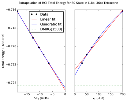
Figure 1: Extrapolation of the HCI total energy to the FCI limit for the lowest singlet state of tetracene in a DZ basis with an (18e, 36o) active space, using natural orbitals. Previously, we obtained the FCI limit by extrapolating to $\epsilon_{1}=0$, using a rational polynomial function of $\epsilon_{1}=0$, which requires several calculated values. A linear or quadratic fit can yield an extrapolated value that is substantially in error, as shown in the figure on the right. In the present paper, we instead extrapolate to $\Delta E_{2}=0$, as shown on the left. Not only is $\Delta E_{2}$ a more meaningful quantity than $\epsilon_{1}$, it also enables a nearly-linear extrapolation of the total energy. The DMRG energy, used for comparison, is the variational energy with bond dimension 1500 obtained by Hachmann et al Hachmann2006 .

VI Further improvements to HCI

Since our most recent HCI paper ShaHolUmr-JCTC-17 , in which we introduced the semistochastic algorithm for evaluating the HCI perturbative correction to the energy, we have improved the algorithm in several ways. First, we have introduced the ability to employ angular momentum symmetry which is the largest abelian subgroup of the $D_{\infty h}$ point group (for any but the smallest basis sets it has orbitals of a larger number of irreducible representations than for the $D_{2h}$ point group that is commonly used for linear molecules). Second, we have implemented time-reversal symmetry which can be used to perform separate calculations of the singlet and triplet states, thereby reducing the Hilbert space of the problem by nearly a factor of two, and reducing the memory requirement of the Hamiltonian in the variational space by a factor of between two and four.

VI.1 Angular momentum symmetry

For real orbitals the 2-electron integrals have 8-fold permutational symmetry. Hence only slightly more than an eighth of the integrals need to be stored. For linear molecules, the orbitals can be chosen to be eigenstates of the z-component of angular momentum, $\hat{L}_{z}$, and the orbitals are complex. In that case, there is only 4-fold permutational symmetry. However, with the usual choice of phase, the integrals are real, and four of the eight are zero since they violate $L_{z}$ conservation. Hence it is still possible to store only an eighth of the integrals, provided a check is performed to ensure $L_{z}$ conservation. This enables us to use $L_{z}$ symmetry to reduce the storage required for the Hamiltonian without increasing the storage required for the integrals.

VI.2 Time-reversal symmetry

The time-reversal operator exchanges the spin labels of the electrons. States with ${}_{z}=0$ are symmetric/antisymmetric under time reversal if $S$ is even/odd. Consequently the basis states can be chosen to be symmetric or antisymmetric linear combinations of time-reversed pairs of Slater determinants.

Consider two spatial orbital configurations, $I$ and $J$. If a determinant is formed by assigning the $\alpha$ electrons to $I$ and the $\beta$ electrons to $J$, i.e., $\left|I_{\alpha}J_{\beta}\right\rangle$, then its time-reversed partner is $(-1)^{n_{\alpha}(n_{\beta}+1)}\left|J_{\alpha}I_{\beta}\right\rangle$, where $n_{\alpha}$ and $n_{\beta}$ are the number of alpha and beta electrons. Note, $(-1)^{n_{\alpha}(n_{\beta}+1)}$ is always equal to 1 for a system containing an equal number of alpha and beta electrons, so we will ignore this phase from now on. We choose to work in the basis of states $\left\{\left|S_{IJ}\right\rangle\right\}$, where

$$\left|S_{IJ}\right\rangle=\begin{cases}\left|I_{\alpha}J_{\beta}\right\rangle,&{\rm if}\quad I=J;\\ \frac{1}{\sqrt{2}}\left(\left|I_{\alpha}J_{\beta}\right\rangle+z\left|J_{\alpha}I_{\beta}\right\rangle\right),&{\rm if}\quad I\neq J,\end{cases}$$ (10)

where $z$ is the eigenvalue of the time-reversal operator, which is either 1 for even $S$ states and -1 for odd $S$ states. Note that basis states for which $I=J$ can occur only when $z=1$.

The matrix elements between pairs of these time-reversal symmetrized states are straightforwardly evaluated. For example, if $I=J$ and $K\neq L$,

$$\left\langle S_{IJ}\left|\hat{H}\right|S_{KL}\right\rangle = \frac{1}{\sqrt{2}}\left\langle I_{\alpha}J_{\beta}\left|\hat{H}\right|K_{\alpha}L_{\beta}\right\rangle$$ (11)

$$+\frac{z}{\sqrt{2}}\left\langle I_{\alpha}J_{\beta}\left|\hat{H}\right|L_{\alpha}K_{\beta}\right\rangle,$$

whereas if $I\neq J$ and $K\neq L$,

$$\left\langle S_{IJ}\left|\hat{H}\right|S_{KL}\right\rangle = \frac{1}{2}\left\langle I_{\alpha}J_{\beta}\left|\hat{H}\right|K_{\alpha}L_{\beta}\right\rangle$$ (12)

$$+\frac{z}{2}\left\langle J_{\alpha}I_{\beta}\left|\hat{H}\right|K_{\alpha}L_{\beta}\right\rangle$$

$$+\frac{z}{2}\left\langle I_{\alpha}J_{\beta}\left|\hat{H}\right|L_{\alpha}K_{\beta}\right\rangle$$

$$+\frac{1}{2}\left\langle J_{\alpha}I_{\beta}\left|\hat{H}\right|L_{\alpha}K_{\beta}\right\rangle$$

$$= \left\langle I_{\alpha}J_{\beta}\left|\hat{H}\right|K_{\alpha}L_{\beta}\right\rangle$$

$$+z\left\langle J_{\alpha}I_{\beta}\left|\hat{H}\right|K_{\alpha}L_{\beta}\right\rangle.$$

We use time-reversal symmetry only for the variational stage. Upon completion of the variational stage, we convert back to the determinant basis and perform Epstein-Nesbet perturbation theory in this basis.

Using time-reversal symmetrized states has two benefits. First, it shrinks the size of the Hilbert space, so that a larger variational manifold can be treated with a given amount of memory. Second, it allows one to target different symmetries separately. For example, if the ground state is a singlet and the first excited state is a triplet, then one can target the lowest triplet state as a ground state and avoid using the excited-state algorithm.

VII Results

We consider the excited states of two molecules, the carbon dimer and tetracene.

Despite its small size, the carbon dimer has strong multireference character even in its ground state, and has been the focus of many experimental and theoretical studies HydeWollaston1802 ; Wu1991 ; martin1992c2 ; Boggio-Pasqua2000 ; Danovich2004 ; UmrTouFilSorHen-PRL-07 ; Kokkin2007 ; Mahapatra2008 ; Varandas2008 ; TouUmr-JCP-08 ; purwanto2009excited ; Booth2011 ; Shi2011 ; Su2011 ; Wang2011 ; Angeli2012 ; Brooke2013 ; Boschen2014 ; Wouters2014 ; Blunt2015 ; Krechkivska2015 ; Mayhall2015 ; Sharma2015 ; Krechkivska2016 . Here we perform excited-calculations in Dunning’s cc-pVQZ basis dunning1989gaussian to compare to calculations from other methods in the literature. Then, we compute the twelve lowest-lying potential energy surfaces in the larger cc-pV5Z basis, extrapolating to the Full CI limit.

The acenes are promising candidates for efficient solar conversion based on singlet fission Smith2010 ; Zimmerman2010 ; Zimmerman2011 ; Lee2013 ; Smith . Here we compute the three lowest-lying states $-$ two singlets and one triplet $-$ in an active space consisting of 18 pi electrons and either 18 or 36 pi orbitals in up to a cc-pVDZ basis.

All integrals used in these calculations were obtained using the PySCF quantum chemistry package sun2017python .

VII.1 Carbon dimer in cc-pVQZ basis

In order to compare to DMRG and FCIQMC energies in the literature, we first computed the potential energy surfaces of the three lowest ${}^{1}\Sigma_{g}^{+}$ and two lowest ${}^{5}\Sigma_{g}$ states in the cc-pVQZ basis with a frozen core. These states were targeted by imposing $L_{z}=0$ ($\Sigma$ states) and using a basis of linear combinations of Slater determinants which is symmetric under time-reversal symmetry (singlets and quintets).

Table 2: Comparison of energies ($E+75$ in Ha) for the three lowest ${}^{1}\Sigma_{g}^{+}$ states of the frozen-core carbon dimer in the cc-pVQZ basis set for three different methods. The DMRG variational energies Sharma2015 used a bond dimension of $M=4000$, and were obtained by simultaneously targeting the three lowest states of ${}^{1}\Sigma_{g}^{+}$ symmetry. The converged values for the DMRG variational energies of the ground state curve (obtained by instead targeting only that single state) are slightly lower than those given here; for example, the equilibrium energy is -75.80269(1) Ha, consistent with the extrapolated HCI total energy. The HCI variational energies were obtained with $\epsilon_{1}=20$ $\mu$Ha, and targeted the lowest five states of either ${}^{1}\Sigma_{g}^{+}$ or ${}^{5}\Sigma_{g}$ symmetry. They used state-averaged natural orbitals, which were obtained from an $\epsilon_{1}=50$ $\mu$Ha variational calculation of the lowest five states in that symmetry sector. Each HCI extrapolation was done using a linear extrapolation with respect to $\Delta E_{2}$ using two runs with $\epsilon_{1}=50$ and 20 $\mu$Ha. The uncertainties in the HCI total energies are 10-20 $\mu$Ha, and reflect both the stochastic uncertainty in the individual points, as well as the error in extrapolation to the FCI limit, taken to be 20% of the difference in energy between the most accurate (smallest $\epsilon_{1}$) calculation and the extrapolated value. The uncertainties in the FCIQMC total energies in Ref. Blunt2015, , range from 1 $\mu$Ha to 13 $\mu$Ha and reflect only the stochastic noise; no attempt was made to extrapolate away the initiator bias.

$R/$Å	DMRG Variational Energy			FCIQMC Energy			HCI Variational Energy			HCI Total Energy
	(Ref. Sharma2015, )			(Ref. Blunt2015, )			(this work)			(this work)
1.0	$-$	$-$	$-$	-0.65570	-0.48665	-0.37654	-0.65598	-0.48688	-0.37692	-0.65620	-0.48716	-0.37725
1.1	-0.76124	-0.62183	-0.50228	-0.76114	-0.62170	-0.50212	-0.76103	-0.62157	-0.50196	-0.76128	-0.62186	-0.50233
1.2	-0.79920	-0.69459	-0.54490	-0.79913	-0.69450	-0.54479	-0.79901	-0.69435	-0.54461	-0.79927	-0.69465	-0.54498
1.24253	-0.80264	-0.71208	-0.54953	-0.80258	-0.71200	-0.54942	-0.80244	-0.71182	-0.54924	-0.80271	-0.71213	-0.54961
1.3	-0.79933	-0.72633	-0.54871	-0.79927	-0.72626	-0.54861	-0.79913	-0.72607	-0.54842	-0.79939	-0.72639	-0.54881
1.4	-0.77965	-0.73267	-0.53776	-0.77961	-0.73261	-0.53766	-0.77945	-0.73240	-0.53746	-0.77973	-0.73274	-0.53789
1.6	-0.72401	-0.70487	-0.51054	-0.72395	-0.70480	-0.51047	-0.72374	-0.70457	-0.51024	-0.72410	-0.70495	-0.51072
1.8	$-$	$-$	$-$	-0.68056	-0.65407	-0.49639	-0.68029	-0.65389	-0.49612	-0.68071	-0.65424	-0.49661
2.0	-0.64552	-0.61469	-0.49290	-0.64548	-0.61470	-0.49297	-0.64522	-0.61453	-0.49269	-0.64565	-0.61486	-0.49316

The HCI variational and total energies are shown in Table 2. Note that even in a relatively large cc-pVQZ basis the variational energies are within 0.5 mHa of the converged total energies for both ground and excited states. The HCI total energies are lower than the (bond dimension 4000) DMRG and FCIQMC energies by 40-260 $\mu$Ha and 120-710 $\mu$Ha respectively. For the ground state, DMRG energies that are in better agreement with HCI energies were obtained Sharma2015 by targeting just the ground state energy, e.g., the equilibrium energy is -75.80269(1) Ha, consistent with the extrapolated HCI total energy. The discrepancy between the FCIQMC energies and the HCI total energies are likely due to the initiator bias in FCIQMC.

VII.2 Carbon dimer in cc-pV5Z basis

We next computed the potential energy surfaces of the twelve lowest-lying states of the carbon dimer in the cc-pV5Z basis:

$$\Sigma_{g} : \quad X^{1}\Sigma_{g}^{+},b^{3}\Sigma_{g}^{-},B^{\prime 1}\Sigma_{g}^{+}$$

$$\Sigma_{u} : \quad c^{3}\Sigma_{u}^{+},1^{1}\Sigma_{u}^{-},2^{3}\Sigma_{u}^{+}$$

$$\Pi_{u} : \quad a^{3}\Pi_{u},A^{1}\Pi_{u}$$

$$\Pi_{g} : \quad d^{3}\Pi_{g},C^{1}\Pi_{g}$$

$$\Delta_{g} : \quad B^{1}\Delta_{g}$$

$$\Delta_{u} : \quad 1^{3}\Delta_{u}$$

Table 3: The twelve lowest-lying potential energy curves ($E+75$ in Ha) of the frozen-core carbon dimer in the cc-pV5Z basis, computed with HCI. Linear extrapolations were performed on two runs with $\epsilon_{1}=100$ and 50 $\mu$Ha, and the uncertainty was reduced by extrapolating with the average slope from all the linear extrapolations of points across a given potential energy surface. The uncertainties in the HCI total energies are approximately 30-50 $\mu$Ha, and include both stochastic error in individual points, as well as error in extrapolation, taken to be 20% of the difference in energy between the most accurate calculation and the extrapolated value.

$R/$Å	$X^{1}\Sigma_{g}^{+}$	$a^{3}\Pi_{u}$	$b^{3}\Sigma_{g}^{-}$	$A^{1}\Pi_{u}$	$c^{3}\Sigma_{u}^{+}$	$B^{1}\Delta_{g}$	$B^{\prime 1}\Sigma_{g}^{+}$	$d^{3}\Pi_{g}$	$C^{1}\Pi_{g}$	$1^{1}\Sigma_{u}^{+/-}$	$1^{3}\Delta_{u}$	$2^{3}\Sigma_{u}^{+/-}$
1.0	-0.66252	-0.58952	-0.50414	-0.55013	-0.64546	-0.46581	-0.49405	-0.54266	-0.48560	-0.47169	-0.28627	-0.31376
1.1	-0.76701	-0.72504	-0.66260	-0.68697	-0.73883	-0.62800	-0.62799	-0.66169	-0.60129	-0.57169	-0.44793	-0.47545
1.2	-0.80461	-0.78657	-0.74165	-0.74986	-0.76505	-0.71040	-0.70037	-0.70862	-0.64496	-0.60667	-0.53547	-0.56209
1.3	-0.80444	-0.80488	-0.77373	-0.76951	-0.75408	-0.74553	-0.73184	-0.71485	-0.64848	-0.60560	-0.57848	-0.60277
1.4	-0.78460	-0.79879	-0.77864	-0.76481	-0.72483	-0.75322	-0.73799	-0.70009	-0.65680	-0.58606	-0.59644	-0.61543
1.5	-0.75663	-0.77988	-0.76845	-0.74736	-0.69009	-0.74566	-0.72893	-0.67759	-0.66995	-0.55851	-0.60848	-0.61240
1.6	-0.72895	-0.75524	-0.75062	-0.72416	-0.65898	-0.73027	-0.70975	-0.65710	-0.67153	-0.62366	-0.61900	-0.61493
1.7	-0.70582	-0.72897	-0.72953	-0.69951	-0.63623	-0.71147	-0.68417	-0.64216	-0.66652	-0.62777	-0.62295	-0.61793
1.8	-0.68550	-0.70334	-0.70780	-0.67575	-0.62333	-0.69188	-0.65860	-0.63000	-0.65797	-0.62692	-0.62214	-0.61352
1.95	-0.65837	-0.66874	-0.67677	-0.64456	-0.61498	-0.66407	-0.62720	-0.61373	-0.64270	-0.62083	-0.61609	-0.59905
2.1	-0.63561	-0.64012	-0.64963	-0.62025	-0.60665	-0.64009	-0.60572	-0.60043	-0.62760	-0.61257	-0.60767	-0.58904
2.4	-0.60433	-0.60182	-0.60940	-0.59236	-0.59148	-0.60643	-0.58535	-0.58525	-0.60404	-0.59723	-0.59205	-0.57999

Besides spatial symmetry, time-reversal symmetry was used to further reduce the size of the Hilbert space by targeting singlets (or quintets) and triplets separately. Thus, for example, the three $\Sigma_{g}$ states were computed in two runs: one which targeted the two lowest-energy singlets and one which target only the lowest energy triplet.

To accelerate convergence of the HCI total energy with respect to $\epsilon_{1}$, HCI natural orbitals were used. Within each of the spatial symmetry sectors, the natural orbitals corresponding to the state-averaged 1-RDM of the lowest variational states of interest were computed. Thus, at each geometry, ten sets of natural orbitals were computed, one for each of the ten spatial symmetry sectors. After the natural orbitals were obtained, for each of the ten symmetry sectors, at each geometry, at least two HCI runs were performed with those natural orbitals in order to enable extrapolation to the FCI limit.

Each HCI calculation was performed starting from a single basis state of the target irreducible representation, found automatically using the following algorithm. First, estimate the global lowest-energy determinant by filling the orbitals with the lowest one-body integrals; this is the current best guess for a good HCI starting state. Next, repeat the following step until convergence: Replace the current HCI starting state with the basis state of the target irreducible representation with lowest energy out of the set of states which are no more than a double excitation away from the current HCI starting basis state.

Although this algorithm does not necessarily result in either the lowest-energy basis state of the target symmetry sector, or the one with maximum overlap with the Full CI ground state, it resulted in a good enough starting point for the HCI runs in this paper.

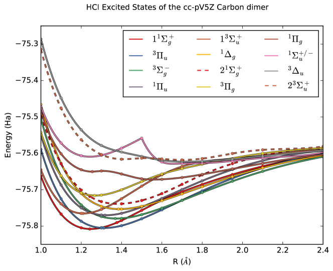
Figure 2: The twelve lowest-lying potential energy surfaces of the carbon dimer in the cc-pV5Z basis, computed using HCI (E+75 in Ha). Time-reversal and $L_{z}$ symmetry were used, and cores were frozen. At each geometry, ten HCI runs were performed, targeting either the one or two lowest states in each of the ten symmetry sectors. The dotted lines correspond to the states that were computed using the excited state algorithm, while the solid lines were computed using the ground state algorithm. The cusp in the ${}^{1}\Sigma_{u}$ curve is due to a curve crossing between the ${}^{1}\Sigma_{u}^{+}$ and ${}^{1}\Sigma_{u}^{-}$ curves near $r=1.5$ Å.

The energies of these twelve states are shown in Table 3 and Fig. 2. In addition the excitation energies of the eight lowest-lying excited states, as shown in Table 4. These excitation energies have a mean absolute deviation of 0.02 eV relative to the experimental values.

		Excitation energy (eV)
State	$R_{\rm eq}/$ Å	Calculated	Experimental
$X^{1}\Sigma_{g}^{+}$	1.24253	0	0
$a^{3}\Pi_{u}$	1.312	0.07	0.09
$b^{3}\Sigma_{g}^{-}$	1.369	0.78	0.80
$A^{1}\Pi_{u}$	1.318	1.03	1.04
$c^{3}\Sigma_{u}^{+}$	1.208	1.16	1.13
$B^{1}\Delta_{g}$	1.385	1.49	1.50
$B^{\prime 1}\Sigma_{g}^{+}$	1.377	1.90	1.91
$d^{3}\Pi_{g}$	1.266	2.50	2.48
$C^{1}\Pi_{g}$	1.255	4.29	4.25

Table 4: Excitation energies of various states of the carbon dimer, calculated with the cc-pV5Z basis set with a frozen core. As in previous DMRG studies Sharma2015 , the bond length for the ${}^{1}\Sigma_{g}^{+}$ ground state was taken from FCIQMC in the cc-pVQZ basis Booth2011 , while the other bond lengths were taken chosen to be the experimental values martin1992c2 . Errors in the calculated excitation energies (relative to Full CI) are smaller than 1 meV. The difference between the calculated and experimental excitation energies could be due to basis set incompleteness, core correlation, relativistic effects, or the interpretation of the experimental data.

VII.3 Tetracene: complete active space calculations

Singlet fission is a promising phenomenon that could enable more efficient solar energy conversion. A photon excites a singlet ground state to a singlet excited state, which quickly “fissions” into two lower-energy triplet excited states, thus enabling a single photon to excite two electrons. The acenes and their derivatives appear to be among the most promising candidates to harness this phenomenon.

As a final application in this paper, we performed complete active space (CAS) calculations in three ways: with a (18e, 18o) pi-orbital active space and either the STO-3G or DZ basis, and with a (18e, 36o) active space containing a double-pi-orbital manifold in the DZ basis. All calculations were performed at the ground state singlet geometry optimized at the UB3LYP/6-31G(d) level of theory.

		Excitation energy (eV)
Basis	Active space	${}^{3}B_{2u}$	${}^{1}B_{2u}$	$2^{1}A_{g}$
STO-3G	(18e, 18o)	1.867(3)	6.34(1)	4.444(3)
DZ	(18e, 18o)	1.8346(4)	4.215(2)	4.3182(4)
DZ	(18e, 36o)	1.67(2)	4.37(2)	4.01(3)

Table 5: Tetracene excitation energies (in eV) relative to the $1^{1}A_{g}$ ground state, calculated using different basis sets and active spaces. In each case, the pi electrons were chosen to be active, and either a singly- (18o) or doubly-complete (36o) set of active pi orbitals were used. Each energy was obtained by an extrapolation with respect to $\Delta E_{2}$ using five different $\epsilon_{1}$ values. A quadratic fit was used to extrapolate to the CAS limit ($\Delta E_{2}=0$). The geometry of the tetracene molecule is shown above the table. This geometry was optimized for the ground (singlet) state, at the UB3LYP/6-31G(d) level of theory, by Hachmann et al Hachmann2006 .

In each basis set/active space, we performed three types of runs: one targeting the lowest two ${}^{1}A_{g}$ states, one targeting the lowest ${}^{3}B_{2u}$ state, and one targeting the lowest ${}^{1}B_{2u}$ state. For each of the three types of runs, natural orbitals were obtained from an HCI run with $\epsilon_{1}=5\times 10^{-5}$ Ha. Then, runs were performed using $\epsilon_{1}$ ranging from $2\times 10^{-4}$ to $2\times 10^{-5}$ Ha, and linear extrapolation to the CASCI limit was performed with respect to $\Delta E_{2}$.

Interestingly, as shown in Table 5, of the three CASCI calculations, only the (18e, 18o) DZ calculation produced the correct ordering of the singlet excited state energies. We believe that dynamical correlation outside of the active space must be included at least perturbatively to obtain more accurate excitation energies. This was also the case for pentacene, as reported by Kurashige and Yanai kurashige2014theoretical . We are currently exploring various methods of including dynamical correlation, including both contracted and uncontracted multireference perturbation theories with HCI as an active space solver.

VIII Conclusions and Outlook

We have presented an efficient excited-state method using Heat-bath Configuration Interaction and a method for extrapolating the resulting energies to the FCI limit. We incorporated symmetries including time-reversal symmetry and angular momentum conservation, enabling us to target excited states in different symmetry sectors. We then used the method to explore the lowest singlet and triplet states in tetracene (relevant to singlet fission) and to calculate twelve low-lying potential energy surfaces of the carbon dimer in the large cc-pV5Z basis.

We are exploring including one more symmetry: the analog of time-reversal symmetry for angular momentum (to separately target $\Sigma^{+}$ and $\Sigma^{-}$ states). For challenging problems, we are also extending our extrapolation procedure to the case where the variational and perturbative steps have different active space sizes, resulting in an extrapolation to the limit of an uncontracted multireference perturbation theory with a complete active space (CAS) reference, rather than to the Full CI limit.

- (1) P. Hohenberg and W. Kohn, Phys. Rev. 136, B864 (1964).
- (2) W. Kohn and L. J. Sham, Phys. Rev. 140, A1133 (1965).
- (3) R. G. Parr and Y. Weitao, Density-functional theory of atoms and molecules, vol. 16 (Oxford university press, 1994).
- (4) F. Coester, Nucl. Phys. 7, 421 (1958).
- (5) J. Čížek, J. Chem. Phys. 45, 4256 (1966).
- (6) J. Čížek and J. Paldus, Physica Scripta 21, 251 (1980).
- (7) G. D. Purvis III and R. J. Bartlett, J. Chem. Phys 76, 1910 (1982).
- (8) J. Geertsen, M. Rittby and R. J. Bartlett, Chem. Phys. Lett. 164, 57 (1989).
- (9) J. F. Stanton and R. J. Bartlett, J. Chem. Phys 98, 7029 (1993).
- (10) M. Nooijen and R. J. Bartlett, J. Chem. Phys. 106, 6441 (1997).
- (11) B. O. Roos, P. R. Taylor and P. E. Siegbahn, Chem. Phys. 48, 157 (1980).
- (12) B. O. Roos, International Journal of Quantum Chemistry 18, 175 (1980).
- (13) P. E. Siegbahn, J. Almlöf, A. Heiberg and B. O. Roos, J. Chem. Phys 74, 2384 (1981).
- (14) B. O. Roos, Advances in Chemical Physics: Ab Initio Methods in Quantum Chemistry Part 2, Volume 69 pp. 399–445 (2007).
- (15) H.-J. Werner and E.-A. Reinsch, J. Chem. Phys. 76, 3144 (1982).
- (16) P. E. Siegbahn, International journal of quantum chemistry 23, 1869 (1983).
- (17) K. Andersson, P. A. Malmqvist, B. O. Roos, A. J. Sadlej and K. Wolinski, J. Phys. Chem. 94, 5483 (1990).
- (18) J. Finley, P.-Å. Malmqvist, B. O. Roos and L. Serrano-Andrés, Chem. Phys. Lett. 288, 299 (1998).
- (19) C. Angeli, R. Cimiraglia, S. Evangelisti, T. Leininger and J.-P. Malrieu, J. Chem. Phys. 114, 10252 (2001).
- (20) C. Angeli, R. Cimiraglia and J.-P. Malrieu, Chem. Phys. Lett. 350, 297 (2001).
- (21) C. Angeli, R. Cimiraglia and J.-P. Malrieu, J. Chem. Phys. 117, 9138 (2002).
- (22) B. Jeziorski and H. J. Monkhorst, Phys. Rev. A 24, 1668 (1981).
- (23) W. D. Laidig and R. J. Bartlett, Chem. Phys. Lett. 104, 424 (1984).
- (24) I. Lindgren, Physica scripta 32, 291 (1985).
- (25) P. A. Malmqvist, A. Rendell and B. O. Roos, J. Phys. Chem. 94, 5477 (1990).
- (26) P. Celani and H.-J. Werner, J. Chem. Phys. 112, 5546 (2000).
- (27) D. Ma, G. Li Manni and L. Gagliardi, J. Chem. Phys. 135, 044128 (2011).
- (28) S. R. White, Phys. Rev. Lett. 69, 2863 (1992).
- (29) S. R. White, Phys. Rev. B 48, 10345 (1993).
- (30) S. R. White and R. L. Martin, J. Chem. Phys. 110, 4127 (1999).
- (31) U. Schollwöck, Rev. Mod. Phys. 77, 259 (2005).
- (32) G. K.-L. Chan and S. Sharma, Annu. Rev. Phys. Chem. 62, 465 (2011).
- (33) G. H. Booth, A. J. W. Thom and A. Alavi, J. Chem. Phys. 131, 054106 (2009).
- (34) D. Cleland, G. H. Booth and A. Alavi, J. Chem. Phys. 132, 041103 (2010).
- (35) F. R. Petruzielo, A. A. Holmes, H. J. Changlani, M. P. Nightingale and C. J. Umrigar, Phys. Rev. Lett. 109, 230201 (2012).
- (36) L. Zhao and E. Neuscamman, J. Chem. Theory Comput. 12, 3436 (2016).
- (37) B. Mussard, E. Coccia, R. Assaraf, M. Otten, C. J. Umrigar and J. Toulouse, arXiv preprint arXiv:1705.09813 (2017).
- (38) P. J. Robinson and E. Neuscamman, arXiv preprint arXiv:1705.04856 (2017).
- (39) F. Schautz and C. Filippi, J. Chem. Phys 120, 10931 (2004).
- (40) W. Purwanto, S. Zhang and H. Krakauer, J. Chem. Phys. 130, 094107 (2009).
- (41) R. Guareschi and C. Filippi, J. Chem. Theory Comput. 9, 5513 (2013).
- (42) N. Blunt, G. H. Booth and A. Alavi, arXiv preprint arXiv:1704.00864 (2017).
- (43) M. Nakata, M. Ehara and H. Nakatsuji, J. Chem. Phys. 116, 5432 (2002).
- (44) D. A. Mazziotti, Accounts of chemical research 39, 207 (2006).
- (45) C. Valdemoro, in Reduced-density-matrix mechanics with applications to many-electron atoms and molecules, edited by D. A. Mazziotti (2007), vol. 134 of Adv. Chem. Phys., pp. 121–164.
- (46) A. A. Holmes, N. M. Tubman and C. J. Umrigar, J. Chem. Theory Comput. 12, 3674 (2016).
- (47) S. Sharma, A. A. Holmes, G. Jeanmairet, A. Alavi and C. J. Umrigar, J. Chem. Theory Comput. 13, 1595 (2017).
- (48) B. Huron, J. Malrieu and P. Rancurel, J. Chem. Phys. 58, 5745 (1973).
- (49) S. Evangelisti, J.-P. Daudey and J.-P. Malrieu, Chem. Phys. 75, 91 (1983).
- (50) C. F. Bender and E. R. Davidson, Phys. Rev. 183, 23 (1969).
- (51) J. Whitten and M. Hackmeyer, J. Chem. Phys 51, 5584 (1969).
- (52) R. J. Buenker and S. D. Peyerimhoff, Theor. Chim. Acta 35, 33 (1974).
- (53) R. Cimiraglia, J. Chem. Phys 83, 1746 (1985).
- (54) R. Cimiraglia and M. Persico, J. Comp. Chem. 8, 39 (1987).
- (55) P. J. Knowles, Chem. Phys. Lett. 155, 513 (1989).
- (56) R. J. Harrison, J. Chem. Phys. 94, 5021 (1991).
- (57) A. Povill, J. Rubio and F. Illas, Theor. Chim. Acta 82, 229 (1992).
- (58) M. M. Steiner, W. Wenzel, K. G. Wilson and J. W. Wilkins, Chem. Phys. Lett. 231, 263 (1994).
- (59) V. García, O. Castell, R. Caballol and J. Malrieu, Chem. Phys. Lett. 238, 222 (1995).
- (60) W. Wenzel, M. Steiner and K. G. Wilson, Int. J. Quantum Chem. 60, 1325 (1996).
- (61) F. Neese, J. Chem. Phys. 119, 9428 (2003).
- (62) H. Nakatsuji and M. Ehara, J. Chem. Phys. 122, 194108 (2005).
- (63) M. L. Abrams and C. D. Sherrill, Chem. Phys. Lett. 412, 121 (2005).
- (64) L. Bytautas and K. Ruedenberg, Chem. Phys. 356, 64 (2009).
- (65) R. Roth, Phys. Rev. C 79, 064324 (2009).
- (66) F. A. Evangelista, J. Chem. Phys. 140, 054109 (2014).
- (67) P. J. Knowles, Mol. Phys. 113, 1655 (2015).
- (68) J. B. Schriber and F. A. Evangelista, J. Chem. Phys. 144, 161106 (2016).
- (69) W. Liu and M. R. Hoffmann, J. Chem. Theory Comput. 12, 1169 (2016).
- (70) T. Zhang and F. A. Evangelista, J. Chem. Theory Comput. 12, 4326 (2016).
- (71) A. Scemama, T. Applencourt, E. Giner and M. Caffarel, J. Comp. Chem. 37, 1866 (2016).
- (72) Y. Garniron, A. Scemama, P.-F. Loos and M. Caffarel, arXiv preprint arXiv:1703.05347 (2017).
- (73) E. Giner, C. Angeli, Y. Garniron, A. Scemama and J.-P. Malrieu, J. Chem. Phys. 146, 224108 (2017).
- (74) P. S. Epstein, Phys. Rev. 28, 6956 (1926).
- (75) R. K. Nesbet, Proc. R. Soc. London, Ser. A. 230, 312 (1955).
- (76) A. J. Walker, ACM Trans. on Math. Software (TOMS) 3, 253 (1977).
- (77) R. A. Kronmal and A. V. Peterson Jr, Amer. Statist. 33, 214 (1979).
- (78) A. A. Holmes, H. J. Changlani and C. J. Umrigar, J. Chem. Theory Comput. (2016).
- (79) J. Hachmann, W. Cardoen and G. K. L. Chan, J. Chem. Phys. 125, 144101 (2006).
- (80) W. Hyde Wollaston, Phil. Trans. R. Soc. London 92, 365 (1802).
- (81) C. J. Wu and E. A. Carter, J. Phys. Chem. 95, 8352 (1991).
- (82) M. Martin, Journal of Photochemistry and Photobiology A: Chemistry 66, 263 (1992).
- (83) M. Boggio-Pasqua, A. I. Voronin, P. Halvick and J. C. Rayez, Journal of Molecular Structure: THEOCHEM 531, 159 (2000).
- (84) D. Danovich, F. Ogliaro, M. Karni, Y. Apeloig, D. L. Cooper and S. Shaik, Angewandte Chemie 116, 143 (2004).
- (85) C. J. Umrigar, J. Toulouse, C. Filippi, S. Sorella and R. G. Hennig, Phys. Rev. Lett. 98, 110201 (2007).
- (86) D. L. Kokkin, G. B. Bacskay and T. W. Schmidt, J. Chem. Phys. 126 (2007).
- (87) U. S. Mahapatra, S. Chattopadhyay and R. K. Chaudhuri, J. Chem. Phys. 129 (2008).
- (88) A. J. C. Varandas, J. Chem. Phys. 129 (2008).
- (89) J. Toulouse and C. J. Umrigar, J. Chem. Phys. 128, 174101 (May 7 2008).
- (90) G. H. Booth, D. Cleland, A. J. W. Thom and A. Alavi, J. Chem. Phys. 135, 1 (2011).
- (91) D. Shi, X. Zhang, J. Sun and Z. Zhu, Mol. Phys. 109, 1453 (2011).
- (92) P. Su, J. Wu, J. Gu, W. Wu, S. Shaik and P. C. Hiberty, J. Chem. Theory Comput. 7, 121 (2011).
- (93) R. N. Wang, X. H. Zheng, Z. X. Dai, H. Hao, L. L. Song and Z. Zeng, Physics Letters A 375, 657 (2011).
- (94) C. Angeli, R. Cimiraglia and M. Pastore, Mol. Phys. 110, 2963 (2012).
- (95) J. S. A. Brooke, P. F. Bernath, T. W. Schmidt and G. B. Bacskay, Journal of Quantitative Spectroscopy and Radiative Transfer 124, 11 (2013).
- (96) J. S. Boschen, D. Theis, K. Ruedenberg and T. L. Windus, Theoretical Chemistry Accounts 133, 1 (2014).
- (97) S. Wouters, T. Bogaerts, P. Van Der Voort, V. Van Speybroeck and D. Van Neck, J. Chem. Phys. 140, 241103 (2014).
- (98) N. S. Blunt, S. D. Smart, G. H. Booth and A. Alavi, J. Chem. Phys. 143, 134117 (2015).
- (99) O. Krechkivska, G. B. Bacskay, T. P. Troy, K. Nauta, T. D. Kreuscher, S. H. Kable and T. W. Schmidt, J. Phys. Chem. A 119, 12102 (2015).
- (100) N. J. Mayhall and M. Head-Gordon, J. Phys. Chem. Lett. pp. 1982–1988 (2015).
- (101) S. Sharma, J. Chem. Phys. 142 (2015).
- (102) O. Krechkivska, G. B. Bacskay, B. A. Welsh, K. Nauta, S. H. Kable, J. F. Stanton and T. W. Schmidt, J. Chem. Phys. 144, 144305 (2016).
- (103) T. H. Dunning Jr, J. Chem. Phys. 90, 1007 (1989).
- (104) M. B. Smith and J. Michl pp. 6891–6936 (2010).
- (105) P. M. Zimmerman, Z. Zhang and C. B. Musgrave, Nature Chemistry pp. 1–5 (2010).
- (106) P. M. Zimmerman, F. Bell, D. Casanova and M. Head-gordon, J. Amer. Chem. Soc. pp. 19944–19952 (2011).
- (107) J. Lee, P. Jadhav, M. A. Baldo, J. Lee, P. Jadhav and M. A. Baldo, Appl. Phys. Lett. 033301, 10 (2013).
- (108) M. B. Smith and J. Michl, Annu. Rev. Phys. Chem. 64, 361 (2013).
- (109) Q. Sun, T. C. Berkelbach, N. S. Blunt, G. H. Booth, S. Guo, Z. Li, J. Liu, J. McClain, S. Sharma, S. Wouters et al., arXiv preprint arXiv:1701.08223 (2017).
- (110) Y. Kurashige and T. Yanai, Bulletin of the Chemical Society of Japan 87, 1071 (2014).