Application of the Mixed Time-averaging Semiclassical Initial Value Representation method to Complex Molecular Spectra

Abstract

The recently introduced mixed time-averaging semiclassical initial value representation molecular dynamics method for spectroscopic calculations [M. Buchholz, F. Grossmann, and M. Ceotto, J. Chem. Phys. 144, 094102 (2016)] is applied to systems with up to 61 dimensions, ruled by a condensed phase Caldeira-Leggett model potential. By calculating the ground state as well as the first few excited states of the system Morse oscillator, changes of both the harmonic frequency and the anharmonicity are determined. The method faithfully reproduces blueshift and redshift effects and the importance of the counter term, as previously suggested by other methods. Differently from previous methods, the present semiclassical method does not take advantage of the specific form of the potential and it can represent a practical tool that opens the route to direct ab initio semiclassical simulation of condensed phase systems.

I Introduction

In a recent publication Buchholz et al. (2016) it has been shown that the ideas of time-averaging Elran and Kay (1999); Kaledin and Miller (2003a) and of semiclassical hybrid dynamics Grossmann (2006) can be combined and lead to an accurate description of molecular spectra of an anharmonic system of interest in the presence of an environment. In the present work the performance of the methodology is tested on systems with a much larger total number of degrees of freedom than treated before and we specifically answer the question under which condition a redshift or a blueshift of the spectral line of the anharmonic system oscillator are to be expected.

To this end, we employ a time-dependent approach to spectroscopy, pioneered by Heller Heller (1981a), based on the so-called semiclassical initial value representation (SC-IVR) molecular dynamics introduced by Miller Miller (1970); Heller (1975); Levit and Smilansky (1977); Heller (1981b); Herman and Kluk (1984); Heller (1991); Miller (2001). Ignited by seminal work of Kay in the early 90s Kay (1994a, b, c), the literature has recently seen a flurry of activities in SC-IVRs, and the Herman-Kluk (HK) approximation Herman and Kluk (1984); Grossmann and Xavier Jr. (1998) has turned out to be the semiclassical method of choice of many authors. Miller (1998); Sun and Miller (1999); Thoss et al. (2001); Wang et al. (2001, 2000); Gelabert et al. (2001); Yamamoto et al. (2002); Miller (2005); Liu and Miller (2007a, b); Tao and Miller (2011); Miller (2006); Shalashilin and Child (2004); Kay (2006); Sklarz and Kay (2004); Harabati and Kay (2007); Hochman and Kay (2009); Herman (1994); Makri (1999); Zhang and Pollak (2004, 2005); Shao and Pollak (2006); Pollak and Martin-Fierro (2007); Martin-Fierro and Pollak (2006); Walton and Manolopoulos (1995, 1996); Brewer et al. (1997); Bonella and Coker (2003); Bonella et al. (2005); Harabati et al. (2004); Grossmann (1999); Viscondi and de Aguiar (2011); Antipov et al. (2015); Venkataraman (2001); Nakamura et al. (2016); Kondorskiy and Nanbu (2015); Tatchen and Pollak (2009); Huo and Coker (2011); Church et al. (2017) More recently, semiclassical molecular dynamics has been implemented for on-the-fly simulations employing ab initio molecular dynamics tools. Ceotto et al. (2009a, b, 2011a, 2013); Conte et al. (2013); Tatchen and Pollak (2009); Ianconescu et al. (2013); Wong et al. (2011); Wehrle et al. (2014, 2015); Zimmermann and Vaníček (2012, 2014)

The HK SC-IVR can, however, be only applied to a relatively small number of coupled degrees of freedom. One route towards the description of the spectra of larger systems is the addition of a time-averaging filter to the phase space integration. Kaledin and Miller (2003a, b) When the filter is fully exploited by taking long time-evolved classical trajectories, the phase space integration numerical effort is reduced by an order of magnitude. Further improvement in computational cost to just a handful of classical trajectories is achieved by taking into consideration that accurate eigenvalues can be obtained from single trajectories when these are close in energy to the eigenvalues. In fact, the trajectories whose energies are about the same as the vibrational peaks’ energies are contributing most to the spectroscopic signal. This approach is called Multiple Coherent TA-SCIVR (MC-SCIVR or MC-TA-SCIVR) and it has proved to be accurate for molecules such as H₂O, CH₄, CH₂D₂ and NH₃. Di Liberto and Ceotto (2016); Tamascelli et al. (2014); Conte et al. (2013); Ceotto et al. (2009a) The significant reduction in number of classical trajectories offered by the MC-TA-SCIVR approach allowed to obtain quite accurate power spectra of molecules using a direct ab initio dynamics simulation, also called on-the-fly or direct ab initio semiclassical dynamics. Gabas et al. (2017); Di Liberto and Ceotto (2016); Tamascelli et al. (2014); Conte et al. (2013); Ceotto et al. (2013, 2011b, 2011a, 2010, 2009a, 2009b) More recently, to beat the curse of dimensionality, a projection technique for the MC-TA-SCIVR has been introduced. The new method is called Divide-and-Conquer SCIVR (DC SCIVR) and it allows the calculation of power spectra for high dimensional systems, such as a fullerene buckyball molecule. Ceotto et al. (2017).

An alternative approach to reduce the number of classical trajectories is Heller’s thawed Gaussian wavepacket dynamics (TGWD) Heller (1975), where only a single Gaussian wavepacket with time-dependent width is propagated. This numerically very cheap method is accurate only for at most harmonic potentials, but it can be combined with the more demanding HK method in the semiclassical hybrid dynamics formalism. Grossmann (2006) Propagating only few degrees of freedom on the HK level, while using the simpler TGWD for the larger environmental part, gives rise to an accurate yet efficient description for the dynamics of systems with many degrees of freedom. We have recently combined the hybrid idea with the time-averaging filter to arrive at the mixed TA-SCIVR method (M-TA-SCIVR) that needs fewer trajectories for convergence than a full TA-SCIVR treatment while being just as accurate for the HK degrees of freedom. Buchholz et al. (2016)

A model system that allows for an easy distinction of degrees of freedom to be treated on the HK versus TGWD level is the one used by Caldeira and Leggett (CL) in their seminal path integral studies of quantum dissipation Caldeira and Leggett (1981). This model with different analytical forms of spectral density and cutoff has been widely used in different branches of the quantum dynamics community to model system-bath interactions. Pollak (1986); Grossmann (1995); Cao (1997); Weiss (1999); Gelabert et al. (2001); Tanimura (2006); Bonfanti et al. (2012); Garashchuk et al. (2013) Using a normal mode analysis, E. Pollak and coworkers have shown analytically for a harmonic system with and without an additional cubic term that the system frequency shift induced by the CL bath with an Ohmic spectral density is always towards higher frequencies, i.e., a blueshift Levine et al. (1988); Pollak (1986). For the cubic system, another analytical study has also shown a blueshift tendency for different bath spectral densities Williams and Loring (1999). The same result has been obtained for a Morse oscillator coupled to a CL bath Joutsuka and Ando (2011). On the other hand, arguing that experimental results often report a redshift of the system frequency (for example for iodine in rare gas matricesKaravitis et al. (2001); Karavitis and Apkarian (2004)), Georgievskii and Stuchebrukhov Georgievskii and Stuchebrukhov (1990) have investigated the influence of the CL counter term on a cubic system potential and found that by omitting the counter term, both blueshift and redshift are possible depending on bath parameters. We will employ a discretized Ohmic spectral density, frequently applied in the CL model, and explicitly treat the dynamics of the combined system, comprising the anharmonic system of interest as well as the bilinearly coupled harmonic bath modes. For up to ten bath degrees of freedom, this can still be done on the Herman-Kluk level of the semiclassical description and serves as a benchmark for our more approximate mixed semiclassical time-averaging method that has to be used if up to 60 bath degrees of freedom are taking part in the dynamics. Studying both cases of a non-resonant as well as a resonant bath, we will show that both redshifts as well as blueshifts are observed.

The paper is organized in the following way: Section II recalls the mixed time-averaging semiclassical method for the calculation of molecular spectra. In Section III, we recapitulate the CL model and discuss the discretization of the bath’s spectral density. In the central Section IV results are first given for ten bath oscillators and different levels of approximation. The high quality of the results of our proposed approximation methodology is thereby shown. Then a detailed study of the frequency shift of the oscillator of interest in the presence of a substantial number of bath degrees of freedom is performed. Conclusions are drawn and an outlook is given in Section V.

II Mixed Time-averaging Semiclassical Initial Value Representation

We first recapitulate the mixed time-averaging semiclassical initial value approach to the calculation of molecular spectra. This method has been introduced recently Buchholz et al. (2016) and combines the semiclassical hybrid dynamics Grossmann (2006) with time-averaging Elran and Kay (1999); Kaledin and Miller (2003a).

The goal of the method is to calculate the power spectrum $I(E)$ of a given initial state $\left|\chi\right\rangle$ subject to a Hamiltonian $\hat{H}$,

$$I(E)=\sum\limits_{n}\left|\left\langle\chi|\psi_{n}\right\rangle\right|^{2}\delta\left(E-E_{n}\right),$$ (1)

where $E_{n}$ are the eigenenergies of interest and $\left|\psi_{n}\right\rangle$ are the corresponding eigenfunctions of $\hat{H}$. The spectrum can be found from the system’s dynamics by expressing the Delta function as a Fourier integral. Eq. (1) then becomes

$$I(E)=\frac{1}{2\pi\hbar}\int\limits_{-\infty}^{\infty}\text{d}t\ \text{e}^{\text{i}Et/\hbar}\left\langle\chi\middle|\text{e}^{-\text{i}\hat{H}t/\hbar}\middle|\chi\right\rangle$$ (2)

The time evolution in Eq. (2) is calculated semiclassically with the propagator by Herman and Kluk Herman and Kluk (1984),

$$\text{e}^{-\text{i}\hat{H}t/\hbar}=\frac{1}{(2\pi\hbar)^{F}}\int\text{d}\mathbf{p}(0)\int\text{d}\mathbf{q}(0)\ C_{t}(\mathbf{p}(0),\mathbf{q}(0))\ \text{e}^{\text{i}S_{t}(\mathbf{p}(0),\mathbf{q}(0))/\hbar}\left|\mathbf{p}(t),\mathbf{q}(t)\right\rangle\left\langle\mathbf{p}(0),\mathbf{q}(0)\right|,$$ (3)

where $(\mathbf{p}(t),\mathbf{q}(t))$ is the $2F$-dimensional classical trajectory evolving from initial conditions $(\mathbf{p}(0),\mathbf{q}(0))$, and $S_{t}$ is the corresponding classical action. Eq. (3) also contains the HK prefactor,

$$C_{t}(\mathbf{p}(0),\mathbf{q}(0))=\sqrt{\frac{1}{2^{F}}\text{det}\left[\frac{\partial\mathbf{q}(t)}{\partial\mathbf{q}(0)}+\frac{\partial\mathbf{p}(t)}{\partial\mathbf{p}(0)}-\text{i}\hbar\boldsymbol{\gamma}\frac{\partial\mathbf{q}(t)}{\partial\mathbf{p}(0)}+\frac{\text{i}}{\hbar\boldsymbol{\gamma}}\frac{\partial\mathbf{p}(t)}{\partial\mathbf{q}(0)}\right]}$$ (4)

which accounts for second-order quantum delocalizations around the classical paths. Finally, the coherent state basis set in position representation for many degrees of freedom is given by the direct product of one-dimensional coherent states,

$$\left\langle\mathbf{x}|\mathbf{p},\mathbf{q}\right\rangle=\left(\frac{\det(\boldsymbol{\gamma})}{\pi^{F}}\right)^{1/4}\exp\left[-\frac{1}{2}\left(\mathbf{x}-\mathbf{q}\right){}^{\text{T}}\boldsymbol{\gamma}\left(\mathbf{x}-\mathbf{q}\right)+\frac{\text{i}}{\hbar}\mathbf{p}^{\text{T}}\left(\mathbf{x}-\mathbf{q}\right)\right]$$ (5)

where $\boldsymbol{\gamma}$ is a diagonal matrix containing $F$ time independent width parameters.

While the semiclassical approximation of the propagator in Eq. (3) in principle allows for the inclusion of an arbitrary number of DOFs, practical applications are limited by the need to converge the phase space integral. Therefore, we will now present two methods that are aimed at accelerating the numerical Monte Carlo phase space integration of Eq. (3). The first step is the introduction of a time averaging integral Elran and Kay (1999); Kaledin and Miller (2003a), which is applied to Eq. (2) and yields a semiclassical approximation with a pre-averaged phase space integrand,

$$\begin{split}I(E)=&\frac{1}{\left(2\pi\hbar\right)^{F}}\int\text{d}\mathbf{p}(0)\int\text{d}\mathbf{q}(0)\frac{1}{\pi\hbar T}\ \text{Re}\int\limits_{0}^{T}\text{d}t_{1}\int\limits_{t_{1}}^{T}\text{d}t_{2}\ C_{t_{2}}(\mathbf{p}(t_{1}),\mathbf{q}(t_{1}))\\ &\times\left\langle\chi\middle|\mathbf{p}(t_{2}),\mathbf{q}(t_{2})\right\rangle\text{e}^{\text{i}\left[S_{t_{2}}\left(\mathbf{p}(0),\mathbf{q}(0)\right)+Et_{2}\right]/\hbar}\left[\left\langle\chi\middle|\mathbf{p}(t_{1}),\mathbf{q}(t_{1})\right\rangle\text{e}^{\text{i}\left[S_{t_{1}}\left(\mathbf{p}(0),\mathbf{q}(0)\right)+Et_{1}\right]/\hbar}\right]^{*}\end{split}$$ (6)

In order to recover a single time integration as in Eq. (2), Kaledin and Miller have suggested the so-called separable approximation Kaledin and Miller (2003a), where the prefactor is written as $C_{t_{2}}(\mathbf{p}(t_{1}),\mathbf{q}(t_{1}))\approx\exp\left[\text{i}(\phi(t_{2})-\phi(t_{1}))/\hbar\right]$, and $\phi(t)/\hbar=\text{phase}\left[C_{t}(\mathbf{p}(0),\mathbf{q}(0))\right]$. This procedure is exact in the harmonic limit and results in the expression

$$I(E)=\frac{1}{\left(2\pi\hbar\right)^{F}}\frac{1}{2\pi\hbar T}\int\text{d}\mathbf{p}(0)\int\text{d}\mathbf{q}(0)\left|\int\limits_{0}^{T}\text{d}t\left\langle\chi\middle|\mathbf{p}(t),\mathbf{q}(t)\right\rangle\text{e}^{\text{i}\left[S_{t}\left(\mathbf{p}(0),\mathbf{q}(0)\right)+Et+\phi_{t}\left(\mathbf{p}(0),\mathbf{q}(0)\right)\right]/\hbar}\right|^{2}$$ (7)

which contains only a single and positive-definite phase space integrand that is expected to be more stable numerically than the two-time integration in Eq. (6). While clearly less computationally demanding than Eq. (6), the separable approximation in Eq. (7) has also turned out to be very accurate for a number of molecular dynamics applications. Kaledin and Miller (2003a, b); Ceotto et al. (2011b); Gabas et al. (2017); Di Liberto and Ceotto (2016); Buchholz et al. (2016); Tamascelli et al. (2014); Conte et al. (2013); Ceotto et al. (2013); Zhuang et al. (2013); Ceotto et al. (2011a, 2010, 2009a, 2009b)

The second step towards making the dynamics of larger systems accessible is to invoke the mixed approximation. To this end, we use the semiclassical hybrid dynamics idea to divide the $2F$ phase space variables into $2F_{\text{hk}}$ for the system space and $2F_{\text{tg}}$ for the bath phase space. Only the system part, denoted by the subscript hk, is then treated on the HK level of accuracy, whereas the simpler single-trajectory TGWD approximation is used for the bath DOFs, which are denoted by the subscript tg. This separation is made only for the semiclassical expression, while the underlying classical dynamics is not modified. We now assume a reference state of Gaussian form, $\left|\chi\right\rangle=\left|\mathbf{p}_{\text{eq}},\mathbf{q}_{\text{eq}}\right\rangle$, where $\mathbf{q_{\text{eq}}}$ is the equilibrium position and $\mathbf{p}_{\text{eq}}$ is the momentum corresponding to some eigenenergy. In the mixed approximation, the initial phase space coordinates are

$$\mathbf{p}_{\text{eq}}(0)=\left(\begin{matrix}\mathbf{p}_{\text{hk}}(0)\\ \mathbf{p}_{\text{eq},\>\text{tg}}(0)\end{matrix}\right),\qquad\mathbf{q}_{\text{eq}}(0)=\left(\begin{matrix}\mathbf{q}_{\text{hk}}(0)\\ \mathbf{q}_{\text{eq},\>\text{tg}}(0)\end{matrix}\right).$$ (8)

Only the HK initial conditions $\left(\mathbf{p}_{\text{hk}}(0),\mathbf{q}_{\text{hk}}(0)\right)$ are found by Monte Carlo sampling around $\left(\mathbf{p}_{\text{eq},\>\text{hk}},\mathbf{q}_{\text{eq},\>\text{hk}}\right)$, while the bath starting coordinates are always at the equilibrium positions, $\left(\mathbf{p}_{\text{eq},\>\text{tg}}(0),\mathbf{q}_{\text{eq},\>\text{tg}}(0)\right)=\left(\mathbf{p}_{\text{eq},\>\text{tg}},\mathbf{q}_{\text{eq},\>\text{tg}}\right)$. Since the TGWD is exact for harmonic potentials, this division should accurately reproduce the contributions of weakly coupled bath DOFs close to their potential minimum. With this separation in place, we expand the classical trajectories and the action to first and second order, respectively, in the displacement coordinates of the bath subspace

$$\delta\mathbf{p}_{\text{tg}}=\mathbf{p}_{\text{tg}}(0)-\mathbf{p}_{\text{eq},\>\text{tg}}(0),\qquad\delta\mathbf{q}_{\text{tg}}=\mathbf{q}_{\text{tg}}(0)-\mathbf{q}_{\text{eq},\>\text{tg}}(0).$$ (9)

This approximates the exponent in Eq. (7) such that the phase space integration over the original bath initial conditions $(\mathbf{p}_{\text{tg}}(0),\mathbf{q}_{\text{tg}}(0))$ can be performed analytically as a Gaussian integral. The expanded classical trajectories become

$$\begin{split}\mathbf{p}(t)=&\left(\begin{matrix}\mathbf{p}_{\text{hk}}(t)\\ \mathbf{p}_{\text{tg}}(t)\end{matrix}\right)=\mathbf{p}_{\text{eq}}(t)+\mathbf{m}_{11}(t)\delta\mathbf{p}_{\text{tg}}+\mathbf{m}_{12}(t)\delta\mathbf{q}_{\text{tg}}\\ \mathbf{q}(t)=&\left(\begin{matrix}\mathbf{q}_{\text{hk}}(t)\\ \mathbf{q}_{\text{tg}}(t)\end{matrix}\right)=\mathbf{q}_{\text{eq}}(t)+\mathbf{m}_{21}(t)\delta\mathbf{p}_{\text{tg}}+\mathbf{m}_{22}(t)\delta\mathbf{q}_{\text{tg}},\end{split}$$ (10)

and the action is

$$\begin{split}S_{t}\left(\mathbf{p}\left(0\right),\mathbf{q}\left(0\right)\right)&=S_{t}\left(\mathbf{p}_{\text{hk}}\left(0\right),\mathbf{q}_{\text{hk}}\left(0\right),\mathbf{p}_{\text{eq},\>\text{tg}}\left(0\right),\mathbf{q}_{\text{eq},\>\text{tg}}\left(0\right)\right)\\ &+\mathbf{p}_{\text{eq}}^{\text{T}}(t)\mathbf{m}_{21}\left(t\right)\delta\mathbf{p}_{\text{tg}}+\left(\mathbf{p}_{\text{eq}}^{\text{T}}(t)\mathbf{m}_{22}\left(t\right)-\mathbf{p}_{\text{eq},\>0,\>\text{tg}}^{\text{T}}\right)\delta\mathbf{q}_{\text{tg}}\\ &+\frac{1}{2}\delta\mathbf{p}_{\text{tg}}^{\text{T}}\mathbf{m}_{11}^{\text{T}}\left(t\right)\mathbf{m}_{21}\left(t\right)\delta\mathbf{p}_{\text{tg}}+\frac{1}{2}\delta\mathbf{q}_{\text{tg}}^{\text{T}}\mathbf{m}_{12}^{\text{T}}\left(t\right)\mathbf{m}_{22}\left(t\right)\delta\mathbf{q}_{\text{tg}}\\ &+\delta\mathbf{q}_{\text{tg}}^{\text{T}}\mathbf{m}_{12}^{\text{T}}\left(t\right)\mathbf{m}_{21}\left(t\right)\delta\mathbf{p}_{\text{tg}}\end{split}$$ (11)

The $\mathbf{m}_{ij}$ in Eqs. (10) and (11) are non-square $F\times F_{\text{tg}}$ submatrices of the stability matrix,

$$\begin{split}\mathbf{m}_{11}(t)=&\frac{\partial\mathbf{p}_{\text{eq}}(t)}{\partial\mathbf{p}_{\text{eq},\>\text{tg}}(0)},\qquad\mathbf{m}_{12}(t)=\frac{\partial\mathbf{p}_{\text{eq}}(t)}{\partial\mathbf{q}_{\text{eq},\>\text{tg}}(0)},\\ \mathbf{m}_{21}(t)=&\frac{\partial\mathbf{q}_{\text{eq}}(t)}{\partial\mathbf{p}_{\text{eq},\>\text{tg}}(0)},\qquad\mathbf{m}_{22}(t)=\frac{\partial\mathbf{q}_{\text{eq}}(t)}{\partial\mathbf{q}_{\text{eq},\>\text{tg}}(0)}.\end{split}$$ (12)

They will be used only for the TG part of the mixed TA-SCIVR integrand, while the phase $\phi_{t}$ of the HK prefactor still comprises the full $F\times F$ matrices from Eq. (4). After unraveling the modulus in Eq. (7), inserting Eqs. (10) and (11), the phase space integration over the TG DOFs can be performed analytically as a Gaussian integral. This results in the mixed TA-SCIVR expression

$$I(E)= \frac{1}{\left(2\hbar\right)^{F}}\frac{1}{\pi^{F_{\text{hk}}}}\frac{\text{Re}}{\pi\hbar T}\int\text{d}\mathbf{p}_{\text{hk}}\left(0\right)\int\text{d}\mathbf{q}_{\text{hk}}\left(0\right)\int_{0}^{T}\text{d}t_{1}\int_{t_{1}}^{T}\text{d}t_{2}$$

$$\times\text{e}^{\text{i}\left[E\left(t_{1}-t_{2}\right)+\phi_{t_{1}}\left(\mathbf{p}_{\text{eq}}\left(0\right),\>\mathbf{q}_{\text{eq}}\left(0\right)\right)-\phi_{t_{2}}\left(\mathbf{p}_{\text{eq}}\left(0\right),\>\mathbf{q}_{\text{eq}}\left(0\right)\right)+S_{t_{1}}\left(\mathbf{p}_{\text{eq}}\left(0\right),\>\mathbf{q}_{\text{eq}}\left(0\right)\right)-S_{t_{2}}\left(\mathbf{p}_{\text{eq}}\left(0\right),\>\mathbf{q}_{\text{eq}}\left(0\right)\right)\right]/\hbar}$$

$$\times\left\langle\mathbf{p}_{\text{eq},\>\text{hk}},\mathbf{q}_{\text{eq},\>\text{hk}}\middle|\mathbf{p}_{\text{eq},\>\text{hk}}\left(t_{1}\right),\mathbf{q}_{\text{eq},\>\text{hk}}\left(t_{1}\right)\right\rangle\left\langle\mathbf{p}_{\text{eq},\>\text{hk}}\left(t_{2}\right),\mathbf{q}_{\text{eq},\>\text{hk}}\left(t_{2}\right)\middle|\mathbf{p}_{\text{eq},\>\text{hk}},\mathbf{q}_{\text{eq},\>\text{hk}}\right\rangle$$ (13)

$$\times\sqrt{\frac{1}{\det\left(\mathbf{A}\left(t_{1}\right)+\mathbf{A}^{*}\left(t_{2}\right)\right)}}$$

$$\times\left\langle\mathbf{p}_{\text{eq},\>\text{tg}},\mathbf{q}_{\text{eq},\>\text{tg}}\middle|\mathbf{p}_{\text{eq},\>\text{tg}}\left(t_{1}\right),\mathbf{q}_{\text{eq},\>\text{tg}}\left(t_{1}\right)\right\rangle\left\langle\mathbf{p}_{\text{eq},\>\text{tg}}\left(t_{2}\right),\mathbf{q}_{\text{eq},\>\text{tg}}\left(t_{2}\right)\middle|\mathbf{p}_{\text{eq},\>\text{tg}},\mathbf{q}_{\text{eq},\>\text{tg}}\right\rangle$$ (14)

$$\times\mbox{exp}\left\{\frac{1}{4}\left(\mathbf{b}_{t_{1}}+\mathbf{b}_{t_{2}}^{*}\right)^{\text{T}}\left(\mathbf{A}\left(t_{1}\right)+\mathbf{A}^{*}\left(t_{2}\right)\right)^{-1}\left(\mathbf{b}_{t_{1}}+\mathbf{b}_{t_{2}}^{*}\right)\right\},$$

which contains some newly defined expressions, namely, the symmetric $2F_{\text{tg}}\times 2F_{\text{tg}}$ matrix $\mathbf{A}(t)$ with blocks

$$\begin{split}\mathbf{A}_{11}(t)=&\frac{1}{4}\mathbf{m}_{21}^{\text{T}}\left(t\right)\mathbf{\boldsymbol{\gamma}}\mathbf{m}_{21}\left(t\right)+\frac{1}{4\hbar^{2}}\mathbf{m}_{11}^{\text{T}}\left(t\right)\mathbf{\boldsymbol{\gamma}}^{-1}\mathbf{m}_{11}\left(t\right)\\ \mathbf{A}_{12}(t)=&\frac{1}{4}\mathbf{m}_{21}^{\text{T}}\left(t\right)\boldsymbol{\gamma}\mathbf{m}_{22}\left(t\right)+\frac{1}{4\hbar^{2}}\mathbf{m}_{11}^{\text{T}}\left(t\right)\boldsymbol{\gamma}^{-1}\mathbf{m}_{12}\left(t\right)\\ \mathbf{A}_{21}(t)=&\frac{1}{4}\mathbf{m}_{22}^{\text{T}}\left(t\right)\boldsymbol{\gamma}\mathbf{m}_{21}\left(t\right)+\frac{1}{4\hbar^{2}}\mathbf{m}_{12}^{\text{T}}\left(t\right)\boldsymbol{\gamma}^{-1}\mathbf{m}_{11}\left(t\right)\\ \mathbf{A}_{22}(t)=&\frac{1}{4}\mathbf{m}_{22}^{\text{T}}\left(t\right)\boldsymbol{\gamma}\mathbf{m}_{22}\left(t\right)+\frac{1}{4\hbar^{2}}\mathbf{m}_{12}^{\text{T}}\left(t\right)\mathbf{\boldsymbol{\gamma}}^{-1}\mathbf{m}_{12}\left(t\right),\end{split}$$ (15)

and the $2F_{\text{tg}}$-dimensional vector $\mathbf{b}(t)\equiv\left(\mathbf{b}_{1,t}^{\text{T}},\mathbf{b}_{2,t}^{\text{T}}\right)^{\text{T}}$ with subvectors

$$\begin{split}\mathbf{b}_{1,t}^{\text{T}}=&-\frac{1}{2}\left(\mathbf{q}\left(t\right)-\mathbf{q}\left(0\right)\right)^{\text{T}}\left[\mathbf{\boldsymbol{\gamma}}\mathbf{m}_{21}\left(t\right)+\frac{\text{i}}{\hbar}\mathbf{m}_{11}\left(t\right)\right]\\ &-\frac{1}{2\hbar^{2}}\left(\mathbf{p}\left(t\right)-\mathbf{p}\left(0\right)\right)^{\text{T}}\left[\mathbf{\boldsymbol{\gamma}}^{-1}\mathbf{m}_{11}\left(t\right)-\text{i}\hbar\mathbf{m}_{21}\left(t\right)\right]\\ \mathbf{b}_{2,t}^{\text{T}}=&-\frac{1}{2}\left(\mathbf{q}\left(t\right)-\mathbf{q}\left(0\right)\right)^{\text{T}}\left[\mathbf{\boldsymbol{\gamma}}\mathbf{m}_{22}\left(t\right)+\frac{\text{i}}{\hbar}\mathbf{m}_{12}\left(t\right)\right]\\ &-\frac{1}{2\hbar^{2}}\left(\mathbf{p}\left(t\right)-\mathbf{p}\left(0\right)\right)^{\text{T}}\left[\mathbf{\boldsymbol{\gamma}}^{-1}\mathbf{m}_{12}\left(t\right)-\text{i}\hbar\mathbf{m}_{22}\left(t\right)\right].\end{split}$$ (16)

The expressions for $\mathbf{A}(t)$ and $\mathbf{b}(t)$ differ from our first publication on this matterBuchholz et al. (2016), as we have left out two constant imaginary contributions in Eqs. (15) and (16) that cancel out in the phase space integrand in Eq. (13). Another difference to Ref$.\$Buchholz et al., 2016 is that we have explicitly written out the scalar quantity $c_{t}$, which has been defined there and which contained the action as well as the overlap of the TG part with the initial state.

Comparing Eq. (13) to the full HK expressions (6) and (7), we have achieved a reduction in dimensionality of the phase space that has to be sampled over. The loss in accuracy is expected to be minimal, as the bath DOFs that are treated on the TG level are weakly coupled and therefore close to harmonic behavior. Again, we stress that there is no decoupling of the underlying classical dynamics.

While the reduced Monte Carlo sampling is clearly advantageous for numerical efficiency, it has come at the price of reintroducing two time integrations in Eq. (13). The integration itself poses no difficulty, as it is simply a two-dimensional Fourier transformation, but calculating the integrand for $N_{\text{steps}}^{2}$ time steps takes a lot of computational time. Therefore, it is highly desirable to find an expression with only a single time integration. In the spirit of the original separable approximation that lead from Eq. (6) to Eq. (7), we proceed by assuming a form for the TG exponent and the TG prefactor that is exact for the harmonic oscillatorBuchholz et al. (2016). The separable form of the exponent reads

$$\begin{split}&\frac{1}{4}\left(\mathbf{b}_{t_{1}}+\mathbf{b}_{t_{2}}^{*}\right)^{\text{T}}\left(\mathbf{A}\left(t_{1}\right)+\mathbf{A}^{*}\left(t_{2}\right)\right)^{-1}\left(\mathbf{b}_{t_{1}}+\mathbf{b}_{t_{2}}^{*}\right)\\ &\qquad\approx\frac{1}{4}\mathbf{b}_{t_{1}}^{\text{T}}\left(\mathbf{A}\left(t_{1}\right)+\mathbf{A}^{*}\left(t_{1}\right)\right)^{-1}\mathbf{b}_{t_{1}}+\frac{1}{4}\left[\mathbf{b}_{t_{2}}^{\text{T}}\left(\mathbf{A}\left(t_{2}\right)+\mathbf{A}^{*}\left(t_{2}\right)\right)^{-1}\mathbf{b}_{t_{2}}\right]^{*},\end{split}$$ (17)

and the TG prefactor is separated in the fashion of a geometric average,

$$\frac{1}{\sqrt{\det\left(\mathbf{A}\left(t_{1}\right)+\mathbf{A}^{*}\left(t_{2}\right)\right)}}\approx\left(\frac{1}{\det\left(\mathbf{A}\left(t_{1}\right)+\mathbf{A}\left(t_{1}\right)\right)}\right)^{1/4}\left(\frac{1}{\det\left(\mathbf{A}\left(t_{2}\right)+\mathbf{A}\left(t_{2}\right)\right)}\right)^{1/4}.$$ (18)

With that, we arrive at the desired separable mixed TA-SCIVR,

$$I(E)= \ \frac{1}{\left(2\hbar\right)^{F}}\frac{1}{\pi^{F_{\text{hk}}}}\frac{1}{2\pi\hbar T}\int\text{d}\mathbf{p}_{\text{hk}}\left(0\right)\int\text{d}\mathbf{q}_{\text{hk}}\left(0\right)\left|\int_{0}^{T}\text{d}t\>\text{e}^{\text{i}\left[Et+\phi_{t}\left(\mathbf{p}_{\text{eq}}\left(0\right),\>\mathbf{q}_{\text{eq}}\left(0\right)\right)+S_{t}\left(\mathbf{p}_{\text{eq}}\left(0\right),\>\mathbf{q}_{\text{eq}}\left(0\right)\right)\right]/\hbar}\right.$$

$$\times\left\langle\mathbf{p}_{\text{eq},\>\text{hk}},\mathbf{q}_{\text{eq},\>\text{hk}}\middle|\mathbf{p}_{\text{eq},\>\text{hk}}\left(t\right),\mathbf{q}_{\text{eq},\>\text{hk}}\left(t\right)\right\rangle\left\langle\mathbf{p}_{\text{eq},\>\text{tg}},\mathbf{q}_{\text{eq},\>\text{tg}}\middle|\mathbf{p}_{\text{eq},\>\text{tg}}\left(t\right),\mathbf{q}_{\text{eq},\>\text{tg}}\left(t\right)\right\rangle$$ (19)

$$\times\left.\frac{1}{\left[\det\left(\mathbf{A}\left(t\right)+\mathbf{A}^{*}\left(t\right)\right)\right]^{1/4}}\exp\left\{\frac{1}{4}\mathbf{b}_{t}^{\text{T}}\left(\mathbf{A}\left(t\right)+\mathbf{A}^{*}\left(t\right)\right)^{-1}\mathbf{b}_{t}\right\}\right|^{2}$$

As we have seen for two-dimensional and three-dimensional model systemsBuchholz et al. (2016), this approximation reproduces both system and bath peaks precisely when compared with exact quantum dynamics results, and reaches tight convergence within a considerably shorter amount of time than the separable TA-SCIVR from Eq. (7).

In the next section, we show that this high accuracy is also achieved for larger systems, and we then go on to use the mixed approximation to investigate the influence of the Caldeira-Leggett counter term on the frequency shift of an anharmonic Morse system. We note in passing that a linearization along the lines of linearized SC-IVRs (LSC-IVR) is not possible, because we just have a single time-evolution operator in our starting expression (1), while the LSC-IVR is propagating densities. Bonnet (2013); Liu (2015); Liu and Miller (2007b); Liu et al. (2011)

III Model: Morse Oscillator Coupled to a Caldeira-Leggett Bath

In order to test the accuracy of the mixed TA-SCIVR, we use a Morse oscillator coupled bilinearly to a Caldeira-Leggett (CL) bath of harmonic oscillators. The Hamiltonian in atomic units has the form

$$H=\frac{p_{\text{s}}^{2}}{2m_{\text{s}}}+V_{\text{s}}(s)+\sum\limits_{i=1}^{F_{\text{b}}}\left[\frac{p_{i}^{2}}{2}+\frac{1}{2}\omega_{i}^{2}y_{i}^{2}+c_{i}y_{i}\left(s-s_{\text{eq}}\right)+\frac{1}{2}\frac{c_{i}^{2}}{\omega_{i}^{2}}\left(s-s_{\text{eq}}\right)^{2}\right]$$ (20)

where the Morse potential for the system coordinate $s$ is

$$V_{\text{s}}(s)=D_{\text{e}}\left(1-\text{e}^{-\alpha\left(s-s_{\text{eq}}\right)}\right)^{2},$$ (21)

and we take the parameters of molecular iodineOvchinnikov and Apkarian (1996) for the dissociation energy $D_{\text{e}}=0.057\ \text{a.u.}$, for the equilibrium distance $s_{\text{eq}}=5.001\ \text{a.u.}$, and for the range parameter $\alpha=0.983\ \text{a.u.}$ The reduced mass of the Morse oscillator is $m_{\text{s}}=m_{\text{r}}=1.165\times 10^{5}\ \text{a.u.}$ There is an analytic solution for the eigenenergies of the Morse potential which we will need later for comparison,

$$E_{n}=\omega_{\text{e}}\left(n+\frac{1}{2}\right)-\omega_{\text{e}}x_{\text{e}}\left(n+\frac{1}{2}\right)^{2},$$ (22)

where $\omega_{\text{e}}=\alpha/\sqrt{m_{\text{r}}/(2D_{\text{e}})}$ is the frequency of the harmonic approximation to the Morse potential, and $x_{\text{e}}=\omega_{\text{e}}/(4D_{\text{e}})$ is the anharmonicity parameter. For the iodine parameters above, these quantities become $\omega_{\text{e}}=9.724\times 10^{-4}\ \text{a.u.}$ and $x_{\text{e}}=4.264\times 10^{-3}\ \text{a.u.}$

The bath part of the Hamiltonian in Eq. (20) consists of the bath kinetic energy, the bilinear system-bath coupling, where $y_{i}$ denotes the bath DOFs, and the Caldeira-Leggett counter term. The latter is introduced in order to prevent a renormalization of the potential Ingold (2002), and we will look into its influence on the system spectrum in the next section. Following Refs. Wang et al., 2001 and Goletz and Grossmann, 2009, we use an Ohmic spectral density with an exponential cutoff,

$$J_{\text{e}}(\omega)=\eta\omega\text{e}^{-\omega/\omega_{\text{c}}},$$ (23)

with the system-bath coupling strength $\eta$ and a cutoff frequency $\omega_{\text{c}}$. In discretized form, the density is defined as

$$J(\omega)=\frac{\pi}{2}\sum\limits_{i=1}^{F_{\text{b}}}\frac{c_{i}^{2}}{\omega_{i}}\delta(\omega-\omega_{i}),$$ (24)

and the coupling coefficients $c_{i}$ in Eq. (20) are chosen such that it becomes equivalent to the continuous form in the limit of infinitely many bath oscillators,

$$c_{i}^{2}=\frac{2}{\pi}\omega_{i}\frac{J_{\text{e}}(\omega_{i})}{\rho(\omega_{i})},$$ (25)

with the frequency density defined by the condition

$$\int\limits_{0}^{\omega_{i}}\text{d}\omega\ \rho(\omega)=i\qquad\text{for }i=1,\dots,F_{\text{b}}.$$ (26)

Here, we choose it as

$$\rho(\omega)=a\frac{J_{\text{e}}(\omega)}{\omega}$$ (27)

where $a$ is a normalization coefficient to ensure that $i=F_{\text{b}}$ if the largest bath frequency $\omega_{i}=\omega_{\text{max}}$ is chosen in Eq. (26), and it amounts to

$$a=\frac{F_{\text{b}}}{\eta\omega_{\text{c}}}\frac{1}{1-\text{e}^{-\omega_{\text{max}}/\omega_{\text{c}}}}.$$ (28)

With Eqs. (24), (26) and (27), one finds the discrete frequencies as

$$\omega_{i}=-\omega_{\text{c}}\ln\left(1-\frac{i(1-\text{e}^{-\omega_{\text{max}}/\omega_{\text{c}}})}{F_{\text{b}}}\right).$$ (29)

If both the cutoff and the maximum frequency of the bath are chosen much smaller than the system frequency, about $F_{\text{b}}=20$ bath oscillators have been shown to be sufficient to reproduce a continuous bathWang et al. (2001). The semiclassical hybrid approach in particular has already turned out to provide an adequate description for the short-time decay of quantum coherence of this specific system-bath problemGoletz and Grossmann (2009). We also choose this frequency density because it allows to set up a bath containing not only many low-frequency modes, but also a few oscillators with frequencies close to the system frequency. A thorough study comparing different spectral densities with their advantages and drawbacks is given in Ref$.\$Goletz et al., 2010.

IV Results and Discussion

The main objective of this paper is the description of the frequency shift of a Morse oscillator coupled to a CL bath using the mixed TA-SCIVR. In order to demonstrate the very good accuracy of the mixed approach, and in particular the separable approximation, we first discuss results for a ten-dimensional bath where TA HK results according to Eq. (7) can still be found relatively easily. After making this comparison, we will turn to baths with up to 60 DOFs and different bath parameters to show their influence on the system spectrum. A specific focus will be on the role of the CL counter term for the anharmonic spectrum.

We employ two different frequency combinations, one with a resonant maximum frequency, $\omega_{\text{c}}=0.5\ \omega_{\text{s}}$ and $\omega_{\max}=\omega_{\text{s}}$, and a low-frequency bath with $\omega_{\text{c}}=0.1\ \omega_{\text{s}}$ and $\omega_{\max}=0.2\ \omega_{\text{s}}$. We choose two different effective coupling parameters $\eta_{\text{eff}}=\eta/(m_{\text{s}}\omega_{\text{s}})$, namely, $\eta_{\text{eff}}=0.5$ and $\eta_{\text{eff}}=2.0$ for the bath with small cutoff frequency and $\eta_{\text{eff}}=0.1$ and $\eta_{\text{eff}}=0.5$ for the big cutoff. The system DOF initially is at equilibrium with nonzero momentum, $(0,\sqrt{m_{\text{s}}\omega_{\text{s}}})$, while the bath oscillators are located at $(0,0)$ because otherwise the spectrum becomes very noisy due to the huge number of excited bath peaks (for an example with 19 DOFs, see Fig. 3 of Ref. Ceotto et al., 2011b). In general, these simplified initial conditions might not be adequate to describe the system frequency shift because possible anharmonic contributions of the bath DOFs are neglected by a dynamics that explores mainly the harmonic neighborhood of the potential minimum. For the bilinearly coupled, harmonic CL bath, however, the difference in the system frequencies arising from initially excited bath DOFs is negligible. The number of semiclassical time steps is $N_{\text{steps}}=2^{14}$ and their length is $\Delta t=(2\pi/\omega_{\text{e}})/20$, resulting in a frequency resolution of $1.2\times 10^{-6}\ \text{a.u.}$ ($0.55\ \text{cm}^{-1}$).

IV.1 Morse Oscillator Coupled to Ten Harmonic Oscillators

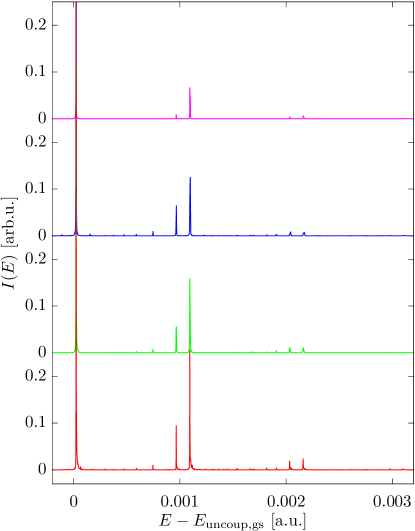
Figure 1: Spectrum of an iodine-like Morse oscillator coupled to a CL bath comprising 10 DOFs with $\omega_{\max}=\omega_{\text{s}}$, $\omega_{\text{c}}=0.5\ \omega_{\text{s}}$ and coupling $\eta_{\text{eff}}=0.5$. From top to bottom: separable TA mixed with 1 HK DOF (magenta) (Eq. (19)), full TA mixed with 1 HK DOF (blue) and full TA mixed with 2 HK DOFs (green) (Eq. (13)), and the separable TA HK (red) using Eq. (6). All spectra are renormalized such that the groundstate peak has height one.

We first discuss an interesting but relatively simple example, the bath comprising ten oscillators with $\omega_{\text{c}}=0.5\ \omega_{\text{s}}$, $\omega_{\max}=\omega_{\text{s}}$, and $\eta_{\text{eff}}=0.5$ (Figs. 1 to 3). In Fig. 1, we give an overview of results obtained with the different methods. The degree of approximation always decreases from top to bottom: the separable mixed approximation according to Eq. (19) is indicated with magenta lines, the full mixed approximation Eq. (13) is blue for one and green for two HK DOFs, and the reference separable TA-SCIVR (Eq. (6) is red. In the full mixed approximation calculations, either only the Morse DOF is treated with HK, or both Morse oscillator and the resonant bath mode, which is expected to experience the strongest anharmonic driving by the system. Only $10^{4}$ trajectories have been used in each case, both to achieve reasonable computational costs and to work out the efficiency of the new methods. In all spectral plots, we subtract the sum of the ground state energies of the individual DOFs,

$$E_{\text{plot}}=E-E_{0}-\sum\limits_{i=1}^{F_{\text{b}}}\frac{\omega_{i}}{2},$$ (30)

in order to make the net effect of the system-bath coupling visible and to facilitate the comparison between baths with different parameters. In Eq$.\$(30), $E_{0}$ is the ground state energy of the Morse oscillator.

Overall, agreement is very good between all methods. Bath peaks are generally not very prominent because there is no initial excitation in the bath; the only dynamics is induced by the system. This is reflected especially in the reference TA-SCIVR and in the full mixed spectra by the fact that the biggest bath peaks are those that correspond to the modes whose frequency is closest to the system. By contrast, just one bath peak from the resonant HO is featured significantly in the separable mixed spectrum.

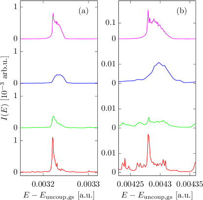
Figure 2: The third (left) and fourth (right) excitation of a Morse oscillator coupled to a CL bath. All bath parameters and plot specifications are identical to Fig. 1.

Fig. 2 highlights some details of the spectra, namely, a zoom into the region of the third and fourth excited system peak. The peaks in these pictures are three to five orders of magnitude smaller than the groundstate and therefore quite noisy, but they can nevertheless be identified as peaks. The full mixed result with one HK DOF clearly disagrees with the reference spectrum. However, this deviation can be removed by treating also the most strongly coupled bath DOF on the HK level of accuracy, which reproduces non-Gaussian distortions of the resonant bath mode. Another way to include these distortions with just one HK DOF might have been to use significantly more trajectories, thus sampling the resonant bath mode indirectly by its coupling to the system mode via the classical dynamics, as discussed in Ref. Buchholz et al., 2012. The separable mixed results for those two peaks agree within the frequency resolution with the reference full HK spectrum. In addition, they are better converged than all the other methods, as can be seen in particular for the fourth excited peak in Fig. 2(b).

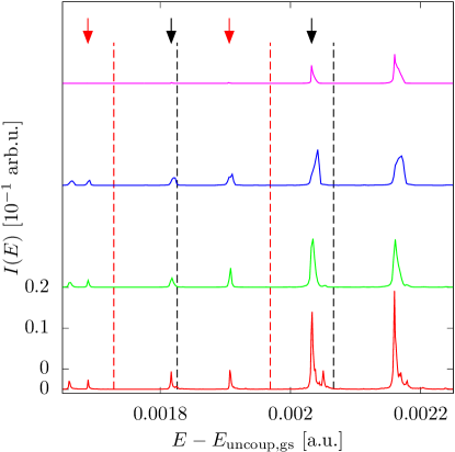
Figure 3: Bath excitations in the spectrum of a Morse oscillator coupled to a CL bath. The respective rightmost peak is the second excitation of the system, the remaining peaks originate from bath modes. All bath parameters and plot specifications are identical to Fig. 1. The arrows in panel designate bath excitations of first order (fundamental) in black color and higher order (overtones) in red color, dashed vertical lines show the respective uncoupled counterpart.

In Fig. 3, we put the bath excitations under the spotlight. The rightmost peak is the second excited state of the system, all remaining peaks are bath excitations (indicated by red and black arrows). The dashed black lines have been obtained by adding the bath frequencies $\omega_{i}$ to the first excited system peak and thus illustrate where these bath peaks would be situated if the bath frequencies remained unchanged by the dynamics. In the same way, the dashed red lines show the expected uncoupled position of higher order bath peaks. The rightmost red line, for example, shows the second excited state of the HO with highest frequency. One sees immediately that each bath peak lies to the left of the respective dashed line, which means that all of these bath oscillators are redshifted. Higher order bath excitations (red color arrows in Fig. 3) are shifted further, as it is expected. As discussed in our first paper on the mixed TA-SCIVR, the separable approximation that leads to Eq. (19) entails a suppression of bath excitations. Consequently, only the first excitation of the highest frequency bath mode shows up significantly in the spectrum. Like the excited states of the Morse oscillator, its position agrees closely with the less approximate results. The other bath excitations are strongly suppressed by the separable mixed method but they can still be identified reliably upon closer inspection and turn out to be also reproduced faithfully.

Due to its numerical advantages, we will perform exclusively separable mixed calculations in the remainder of this paper, where we investigate the system behavior for different bath characteristics.

IV.2 Frequency shifts for different bath sizes and role of the Caldeira-Leggett counter term

Having established that the separable mixed method offers the same accuracy with respect to peak positions as the full HK treatment for the CL system, we now increase the bath size up to 60 bath HOs. Again, we use a very off resonant bath on the one hand and one with bath frequencies up to the system frequency on the other. In addition, we will analyse the influence of the CL counter term on the outcome of the spectral calculations for our examples. We will undertake a similar investigation as previously performed by Georgievskii and Stuchebrukhov Georgievskii and Stuchebrukhov (1990) and therefore look at the CL model in the form of Eq. (20) as well as a Hamiltonian without the counter term,

$$H=\frac{p_{\text{s}}^{2}}{2m_{\text{s}}}+V_{\text{s}}(s)+\sum_{i=1}^{F_{\text{b}}}\left\{\frac{p_{i}^{2}}{2}+\frac{1}{2}\omega_{i}^{2}y_{i}^{2}+c_{i}y_{i}\left(s-s_{\text{eq}}\right)\right\}.$$ (31)

The following numerical investigations will comprise bath sizes of 10, 20, 40, and 60 DOFs, such that convergence with respect to the number of bath HOs can be tested. As we are using the separable mixed TA-SCIVR, we can keep the number of trajectories constant at $10^{4}$ for the differently sized baths. The number of HK DOFs has been either one or two. Especially for the low frequency bath it was sufficient to describe only the Morse oscillator with HK, while in the case of the high bath cutoff it was helpful to include the resonant bath oscillator into the HK part as well.

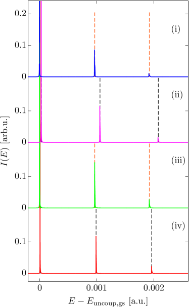
Figure 4: Spectra for a Morse oscillator in a CL bath with 20 HOs for low cutoff frequency. Bath parameters are $\omega_{\text{c}}=0.1\ \omega_{\text{s}}$ and $\omega_{\text{max}}=0.5\ \omega_{\text{s}}$, with effective couplings $\eta_{\text{eff}}=0.5$ (solid red and green lines) and $\eta_{\text{eff}}=2.0$ (magenta and blue). Results (i) and (iii) are from calculations without the CL counter term, (ii) and (iv) from calculations including the CL counter term. The dashed lines represent eigenvalues of a regular 1D Morse potential (black) and of a 1D Morse potential modified by the CL counter term according to Eq. (32) (red).

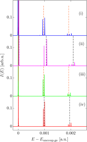
Figure 5: Spectra for a Morse oscillator in a CL bath with 20 HOs for high cutoff frequency. Bath parameters are $\omega_{\text{c}}=0.5\ \omega_{\text{s}}$ and $\omega_{\text{max}}=\omega_{\text{s}}$, with effective couplings $\eta_{\text{eff}}=0.1$ (red and green lines) and $\eta_{\text{eff}}=0.5$ (magenta and blue). All remaining plot specifications as in Fig. 4.

An exemplary overview of results for the different bath parameters is given in Figs. 4 and 5 for a bath with 20 DOFs, where again all spectra are normalized such that the respective most intense peak’s size is one. To illustrate the shift of the Morse spectrum, we plot the analytical eigenvalues of the Morse potential from Eq. (22) for calculations without the CL counter term (see red dashed lines in Figs. 4 and 5). For the evaluation of the calculations with the original CL Hamiltonian in Eq. (20), the one-dimensional reference is modified because the counter term, which does not depend on the bath coordinates, effectively amounts to a renormalization of the system potentialRosenau da Costa et al. (2000). Therefore, in this case we use eigenenergies $E_{\text{mod},n}$ (black dashed lines) of the Morse potential modified by the CL counter term,

$$V_{\text{s},\text{mod}}(s)=D_{\text{e}}\left(1-\text{e}^{-\alpha\left(s-s_{\text{eq}}\right)}\right)^{2}+\frac{\pi}{4}\frac{F_{\text{b}}}{a}\left(s-s_{\text{eq}}\right)^{2}.$$ (32)

The spectra with low bath cutoff frequencies in Fig. 4 exhibit system peaks that are hardly different from the 1D result. If the CL counter term is included (spectra (ii) and (iv)), we see different blueshifts that can be attributed to the modification of the system potential by the counter term. For the cases without counter term (spectra (i) and (iii)), even the difference in effective coupling strength has little effect, at least on the scale of this figure. The higher cutoff frequency, on the other hand, has a much greater impact on the spectra, as depicted in Fig. 5. Instead of just the excited states of the system, the original peak has been split, corresponding to redshifted bath and blueshifted system excitations as discussed in the previous section. Again, the respective rightmost peak of each group belongs to the system excitation, while the others are first and second excited state of the resonant bath mode. The appearance of these bath peaks, or, more to the point, the fact that they are no longer suppressed but show up so prominently here, is due to the fact that the resonant bath mode can be driven much more effectively by the system than the non-resonant one from the low-cutoff example. In addition, the resonant HO is now incorporated into the HK part of the calculation, which does not suppress bath overtones. The more interesting and more relevant feature for us, however, is that the stronger system-bath interaction results in a sizable blueshift of the system both for calculations with and without CL counter term and always relative to the respective modified or unmodified one-dimensional eigenvalues. For low effective system-bath coupling, the difference between the results with and without counter term is not very pronounced (lower graphs in Fig. 5), which seems justified given that the effect of the potential renormalization is almost insignificant. The high coupling case, on the other hand, exhibits a greater blueshift of the system if the counter term is not included. Comparing high and low effective coupling, we see that an increase of $\eta_{\text{eff}}$ leads to a bigger distance between system and bath peaks of the same group as a consequence of an enhancement of the respective trend towards blueshift or redshift.

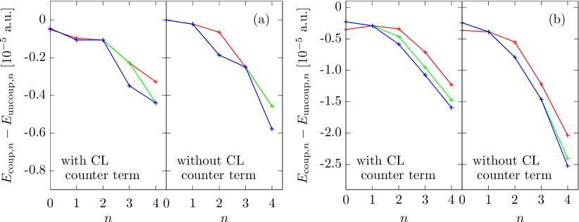
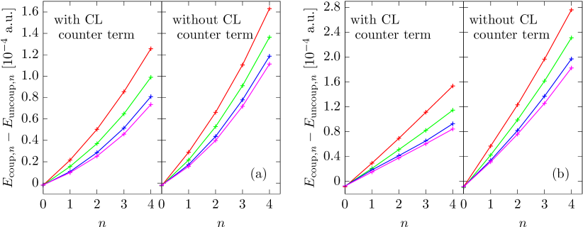
Figure 6: Shift of the eigenenergies of a Morse oscillator coupled to a CL bath with parameters $\omega_{\text{max}}=0.5\ \omega_{\text{s}}$, $\omega_{\text{c}}=0.1\ \omega_{\text{s}}$, and different coupling strengths: $\eta_{\text{eff}}=0.5$ in panel (a) and $\eta_{\text{eff}}=2.0$ in panel (b). The bath comprises either 10 (red crosses), 20 (green), or 40 (blue) HOs, and the solid lines are just a guide to the eye. The CL counter term according to Eq. (20) is included in the calculations on the left side of each panel, and not included on the right side (Eq. (31)). As a consequence, the reference eigenenergies for the 1D MO are different depending on the presence of the counter term, according to Eq. (33).

Figure 7: Shift of the eigenenergies of a MO coupled to a CL bath with parameters $\omega_{\text{max}}=\omega_{\text{s}}$, $\omega_{\text{c}}=0.5\ \omega_{\text{s}}$, and coupling strengths $\eta_{\text{eff}}=0.1$ in panel (a) and $\eta_{\text{eff}}=0.5$ in (b). All plot specifications as in Fig. 7, with the addition of results for 60 bath DOFs (magenta crosses).

For a more detailed quantitative discussion of the system’s blueshift, we take a look at the first five system peaks for each of the different baths (Figs. 7 to 9). In Figs. 7 and 7, the shift of the peak energies is plotted. In a similar way as before, the energy of an appropriate uncoupled reference, now depending on the peak index, is subtracted,

$$E_{\text{plot},n}=E_{\text{coup},n}-\left(E_{\text{s},n}+\sum_{i=1}^{F_{\text{b}}}\frac{\omega_{i}}{2}\right),$$ (33)

where the system eigenenergies $E_{\text{s},n}$ are either the analytic eigenenergies $E_{n}$ of the undisturbed Morse potential from Eq. (21) for the calculations without CL counter term, or the numerically calculated eigenenergies $E_{\text{mod},n}$ of the modified Morse potential from Eq. (32) for the calculations including the counter term. Thus, we visualize the net shift of the peaks, which includes the energy shifts of the system eigenstates and of the bath groundstate. A blueshift of the system is characterized by a sequence of increasing values, whereas a redshift shows the opposite behavior. Assuming that the interaction with the bath only changes the Morse parameters of the system to $\tilde{\omega}_{\text{e}}$ and $\tilde{x}_{\text{e}}$, but not the overall Morse form itself, Eq. (33) should have the form of a parabola, as can be seen by inserting the Morse eigenvalues from Eq. (22),

$$E_{\text{plot},n}=\left(\tilde{\omega}_{\text{e}}-\omega_{\text{e}}\right)\left(n+\frac{1}{2}\right)-\left(\tilde{\omega}_{\text{e}}\tilde{x}_{\text{e}}-\omega_{\text{e}}x_{\text{e}}\right)\left(n+\frac{1}{2}\right)^{2}-\Delta E_{\text{b},\text{gs}}.$$ (34)

The last term in this equation is the change of the bath ground state energy upon coupling to the system, which acts as a constant offset.

As an alternative measure, Figs. 9 and 9 show the difference of consecutive excited Morse peaks, $\tilde{E}_{n}-\tilde{E}_{n-1}$, such that the shift of the bath groundstate energy $\Delta E_{\text{b},\text{gs}}$ drops out. This kind of representation is referred to as Birge-Sponer extrapolation and can be used experimentally to determine Morse potential parameters from spectroscopic data Lewis et al. (1994); David (2008). Based on the analytic formula for the Morse eigenenergies in Eq. (22), a linear fit of these points yields the harmonic approximation frequency $\omega_{\text{e}}$ as the intersection with the vertical axis and the anharmonicity $\omega_{\text{e}}x_{\text{e}}$, which is proportional to the slope of the line. An increase of the slope corresponds to a redshift whereas a decreasing slope means a bigger difference between eigenvalues and therefore a blueshift. We show a linear fit of the first four system energy differences and compare this result to the one-dimensional Morse oscillator or its modified version (black “$\times$”, dashed line), for which the intersection with the vertical axis has also been obtained by Birge-Sponer fit. The shifts of the experimental parameters with respect to the gas phase result are summarized in Tab. 1.

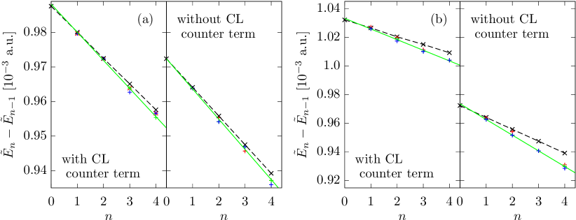
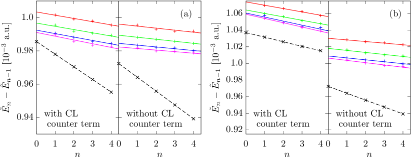
Figure 8: Birge-Sponer fit to the difference of consecutive eigenenergies $\tilde{E}_{n}$ of the Morse oscillator coupled to a low-frequency CL bath from Fig. 7. Bath parameters are $\omega_{\text{max}}=0.5\ \omega_{\text{s}}$, $\omega_{\text{c}}=0.1\ \omega_{\text{s}}$, and couplings are $\eta_{\text{eff}}=0.5$ in panel (a) and $\eta_{\text{eff}}=2.0$ in (b). The “+” crosses denote results with 10 (red), 20 (green), and 40 (blue) bath HOs. The solid green line is a linear fit to the 20 DOFs result, and the dashed black line with “$\times$” crosses is the corresponding 1D MO reference, i.e., $E_{n}-E_{n-1}$ (Eq. (21)) or $E_{\text{mod},n}-E_{\text{mod},n-1}$ (Eq. (32)), respectively.

Figure 9: Birge-Sponer fit to the difference of consecutive eigenenergies $\tilde{E}_{n}$ of the Morse oscillator coupled to a high-frequency CL bath from Fig. 7. Bath parameters are $\omega_{\text{max}}=\omega_{\text{s}}$, $\omega_{\text{c}}=0.5\ \omega_{\text{s}}$, and couplings are $\eta_{\text{eff}}=0.1$ in panel (a) and $\eta_{\text{eff}}=0.5$ in (b). All lines are fits to points of the same color as in Fig. 9, with the color code from Fig. 7.

The analysis is interesting especially for the low-frequency bath, where we could not see much in the overview plot (Fig. 5). Results are presented in Figs. 7 and 9 for calculations with 10 (red crosses), 20 (green crosses), and 40 bath DOFs (blue crosses), and with two different system-bath couplings, $\eta_{\text{eff}}=0.5$ on the left (panel (a)), and for $\eta_{\text{eff}}=2.0$ on the right (panel (b)). Due to the fits in the Birge-Sponer plots in Fig. 9 being almost identical, we have plotted only one line in each case. For low coupling, we see an almost negligible redshift. The effect of the CL counter term is nicely illustrated by the Birge-Sponer plot: the result with counter term is clearly blueshifted with respect to the original Morse eigenvalues, but it is almost on top of the appropriately modified 1D energies. The influence of the system-bath dynamics is much smaller by comparison, especially given that our energy grid resolution is $\Delta E=1.2\times 10^{-6}\ \text{a.u.}$ These findings are corroborated by the calculations with higher system-bath coupling strength. Here, the redshift is much more pronounced, but again, for the original CL potential the main contribution to the energy shift is due to the counter term. For all calculations with low bath cutoff frequency, the number of bath oscillators does not have much impact on the system spectrum. In the low coupling case, the difference between all three bath sizes is one frequency grid point at most. For the higher coupling, 10 bath DOFs influence the system somewhat less than 20 and 40 bath HOs, which yield very similar results. This weak dependence on bath size is of course a consequence of the low cutoff and maximum bath frequencies. While the bath mode with highest frequency is always the same, most additional bath oscillators are far off-resonant. As a conclusion, we can say that we find the same 20 to 40 bath DOFs to be sufficient to describe a continuous bath in this low frequency case, as it has been reported in Ref. Wang et al., 2001.

The case of baths with a high cutoff and resonant maximum frequency is investigated in detail in Figs. 7 and 9. We have used the same color scheme for bath size and reference states, but added calculations with 60 bath DOFs (magenta crosses). The overall behavior of the system is completely different compared to the low-frequency case, with strong blueshifts for each bath setup, as already seen in the overview figure 5. For $\eta_{\text{eff}}=0.1$, the effect of the bath on the system is somewhat bigger without the CL counter term, as shown on the left side of Fig. 7(a). The counter term, which is harmonic in the system coordinate, restricts the system dynamics and thus also the system-bath interaction. If it is left out of the calculation, the system-bath dynamics induces a larger shift of the system frequency. The total blueshift in Fig. 9, on the other hand, is also determined by the change of the 1D eigenenergies by the counter term, which offsets the weaker system-bath dynamics and leads to quite similar overall results in this low-coupling case. Unlike before, the results strongly depend on the bath size, which is quite understandable given that each increase adds in particular some oscillators that are close to the system frequency and notably influence the system’s dynamics. As the differences between results get smaller with each addition of bath HOs, we are approaching convergence with respect to a continuous bath description with 60 bath DOFs. The higher system-bath coupling amplifies these trends. Now, the difference of coupled and uncoupled peak energies (Fig. 7(b)) is almost twice as big for the calculation without CL counter term compared to the one that includes it. However, the modification of the 1D eigenenergies induced by the counter term is so big in this case that the total blueshift (Fig. 9(b)) becomes even larger than without counter term. Again, we can see that the results converge with increasing bath size.

	bath w/o resonant modes		bath w/ resonant modes
with CL counter term	$\tilde{\omega}_{\text{e}}>\omega_{\text{e}}$		$\tilde{\omega}_{\text{e}}>\omega_{\text{e}}$
(Eq. (20))	$\tilde{\omega}_{\text{e}}\tilde{x}_{\text{e}}<\omega_{\text{e}}x_{\text{e}}$		$\tilde{\omega}_{\text{e}}\tilde{x}_{\text{e}}<\omega_{\text{e}}x_{\text{e}}$
without CL counter term	$\tilde{\omega}_{\text{e}}>\omega_{\text{e}}$		$\tilde{\omega}_{\text{e}}>\omega_{\text{e}}$
(Eq. (31))	$\tilde{\omega}_{\text{e}}\tilde{x}_{\text{e}}>\omega_{\text{e}}x_{\text{e}}$		$\tilde{\omega}_{\text{e}}\tilde{x}_{\text{e}}<\omega_{\text{e}}x_{\text{e}}$

Table 1: Change of the harmonic frequency and the anharmonicity of a Morse oscillator in the presence of a Caldeira-Leggett bath. All shifts are relative to the gas phase result.

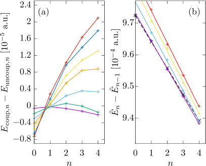
Figure 10: Cutoff frequency dependence of the shift of the eigenenergies of a Morse oscillator coupled to a CL bath. Bath parameters: 20 HOs, maximum frequency fixed at $\omega_{\text{max}}=0.7\ \omega_{\text{s}}$, and cutoff frequencies $\omega_{\text{c}}$ are $0.1\ \omega_{\text{s}}$ (violet “+” crosses), $0.2\ \omega_{\text{s}}$ (green), $0.3\ \omega_{\text{s}}$ (light blue), $0.4\ \omega_{\text{s}}$ (orange), $0.5\ \omega_{\text{s}}$ (yellow), $0.6\ \omega_{\text{s}}$ (dark blue), and $0.7\ \omega_{\text{s}}$ (red). The CL counter term is not included in the Hamiltonian (Eq. (31)). The “$\times$” crosses and black dashed line show the eigenenergy differences of the gas-phase Morse oscillator. The lines in subfigure (a) are just a guide to the eye. In subfigure (b), the lines are the linear fit to the crosses of the same color.

Given the different nature of the system frequency shift in Figs. 7 and 7, one may wonder how the transition from redshift to blueshift looks like for varying bath cutoff or maximum frequency. This is illustrated exemplarily in Figs. 10 and 11 for a bath with 20 HOs and using the Hamiltonian without the CL counter term. In Fig. 10, we keep the maximum frequency fixed at $\omega_{\text{max}}=0.7\ \omega_{\text{s}}$, while the cutoff frequency varies between $\omega_{\text{c}}=0.1\ \omega_{\text{s}}$ and $\omega_{\text{c}}=0.7\ \omega_{\text{s}}$. As expected from the above investigations, the blueshift of the higher eigenfrequencies is gradually diminished and finally turns into a redshift as the bath oscillators become more off-resonant. Taking the parabola from Eq. (34) as an appropriate description for the curves in subfigure (a), we see that indeed all of these graphs display a negative curvature, which is equivalent to an increase and therefore a redshift of the anharmonicity $\tilde{\omega}_{\text{e}}\tilde{x}_{\text{e}}$. This is corroborated by the Birge-Sponer plot in subfigure (b), where it shows as a steeper slope of the linear fit. The harmonic approximation frequency $\tilde{\omega}_{\text{e}}$ is always blueshifted, and the shift is enhanced as $\omega_{\text{c}}$ grows.

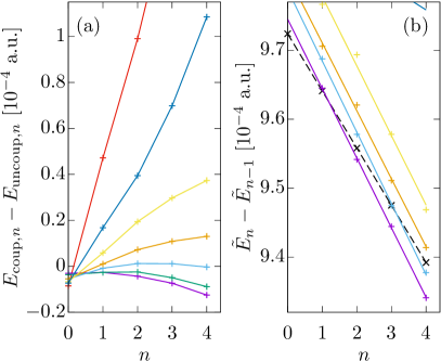
Figure 11: Maximum bath frequency dependence of the shift of the eigenenergies of a Morse oscillator coupled to a CL bath. Bath parameters: 20 HOs, cutoff frequency fixed at $\omega_{\text{c}}=0.5\ \omega_{\text{s}}$, and maximum frequencies $\omega_{\text{max}}$ are $0.4\ \omega_{\text{s}}$ (violet “+” crosses), $0.5\ \omega_{\text{s}}$ (green), $0.6\ \omega_{\text{s}}$ (light blue), $0.7\ \omega_{\text{s}}$ (orange), $0.8\ \omega_{\text{s}}$ (yellow), $0.9\ \omega_{\text{s}}$ (dark blue), and $1.0\ \omega_{\text{s}}$ (red). The CL counter term is not included in the Hamiltonian (Eq. (31)). The “$\times$” crosses and black dashed line show the eigenenergy differences of the gas-phase Morse oscillator. The lines in subfigure (a) are just a guide to the eye. In subfigure (b), the lines are the linear fit to the crosses of the same color.

Similar behavior is observed for the opposite case displayed in Fig. 11, where we keep the cutoff frequency fixed at $\omega_{\text{c}}=0.5\ \omega_{\text{s}}$ and vary the maximum frequency between $\omega_{\text{max}}=0.4\ \omega_{\text{s}}$ and $\omega_{\text{max}}=1.0\ \omega_{\text{s}}$. The parabolas in subfigure (a) now change from negative to positive curvature as the the maximum bath frequency becomes resonant. This indicates a blueshift of the anharmonicity if there are close to resonant modes present in the bath, as already seen in Figs. 7 and 9. As the maximum frequency becomes more off-resonant, we see again a redshift of the anharmonicity. In both cases, the harmonic frequency is shifted to a higher value.

V Conclusions and Outlook

We have shown that the time averaged mixed semiclassical hybrid approach introduced recently Buchholz et al. (2016) can be applied to study spectroscopic signatures of an anharmonic system of interest in a large environment, with up to 60 bath degrees of freedom. Conditions on the bath parameters have been identified, that lead either to a redshift or to a blueshift of the system frequency. We have investigated the cases of a non-resonant and a resonant bath where in the latter case also the bath oscillator closest to resonance was treated on the full HK level. Furthermore, we have compared results from calculations with and without the Caldeira-Leggett counter term to demonstrate that this term causes a large portion of the blueshift which is observed with respect to the gas phase Morse oscillator. If the one-dimensional reference potential is adjusted appropriately with the counter term, the effect of the system-bath interaction on the system eigenenergies is similar for calculations with and without counter term. The change of the system frequency depends both on the bath cutoff and the maximum frequency. In the case of a strongly non-resonant bath, the anharmonicity $\omega_{\text{e}}x_{\text{e}}$ is redshifted. The harmonic frequency $\omega_{\text{e}}$ always shifts to a higher value. If there are at least some bath frequencies close to resonance, on the other hand, the fundamental frequency as well as the anharmonicity are blueshifted. Overall, the mixed time averaged semiclassical hybrid approach demonstrated to be a robust semiclassical approximation that properly accounts for different types of coupling, even for up to 61-dimensional potential. This opens the route of its application to more realistic condensed phase systems than the Caldeira-Leggett potential modeling.

Recently, it has been argued that the modeling of an anharmonic system bilinearly coupled to a harmonic bath suffers the invertibility problem Gottwald et al. (2015). The next goal that we intend to tackle therefore is the study of realistic system bath Hamiltonians with Lennard-Jones type interaction, for systems like iodine in a Krypton matrix, which have also been studied experimentally Karavitis et al. (2001).

Future implementation will include the finite temperature effects and the broadening of the peaks induced by the temperature. Also different types of semiclassical approximation, such as Linearized (LSC-IVR) and van Vleck SC-IVR (VV-SC-IVR), can be equally mixed as it was done for the time-averaging SC-IVR and the TGWD. Eventually, given the cheap computational cost of the time-averaging SC-IVR, the present mixed semiclassical method will be implemented for direct ab initio simulations of condensed phase systems.

VI Acknowledgements

Michele Ceotto and Max Buchholz acknowledge financial support from the European Research Council (ERC) under the European Union’s Horizon 2020 research and innovation programme (Grant Agreement No. [647107] — SEMICOMPLEX — ERC-2014-CoG). M.C. acknowledges also the CINECA and the Regione Lombardia award under the LISA initiative (grant GREENTI) for the availability of high performance computing resources. M. B. acknowledges funding from the Graduate Academy of TU Dresden as well as from the IMPRS of the MPI-PKS Dresden.

References

- Buchholz et al. (2016) M. Buchholz, F. Grossmann, and M. Ceotto, J. Chem. Phys. 144, 094102 (2016).
- Elran and Kay (1999) Y. Elran and K. G. Kay, J. Chem. Phys. 110, 3653 (1999).
- Kaledin and Miller (2003a) A. L. Kaledin and W. H. Miller, J. Chem. Phys. 118, 7174 (2003a).
- Grossmann (2006) F. Grossmann, J. Chem. Phys. 125, 014111 (2006), 10.1063/1.2213255.
- Heller (1981a) E. J. Heller, Acc. Chem. Res. 14, 368 (1981a).
- Miller (1970) W. H. Miller, J. Chem. Phys. 53, 3578 (1970).
- Heller (1975) E. J. Heller, J. Chem. Phys. 62, 1544 (1975).
- Levit and Smilansky (1977) S. Levit and U. Smilansky, Ann. Phys. (N.Y.) 103, 198 (1977).
- Heller (1981b) E. J. Heller, J. Chem. Phys. 75, 2923 (1981b).
- Herman and Kluk (1984) M. F. Herman and E. Kluk, Chemical Physics 91, 27 (1984).
- Heller (1991) E. J. Heller, in Chaos et Physique Quantique/Chaos and Quantum Physics, Proc. Les Houches Summer School, Session LII 1989, edited by M. J. Giannoni, A. Voros, and J. Zinn-Justin (North-Holland, Amsterdam, 1991).
- Miller (2001) W. H. Miller, The Journal of Physical Chemistry A 105, 2942 (2001).
- Kay (1994a) K. G. Kay, J. Chem. Phys. 100, 4377 (1994a).
- Kay (1994b) K. G. Kay, J. Chem. Phys. 100, 4432 (1994b).
- Kay (1994c) K. G. Kay, J. Chem. Phys. 101, 2250 (1994c).
- Grossmann and Xavier Jr. (1998) F. Grossmann and A. L. Xavier Jr., Physics Letters A 243, 243 (1998).
- Miller (1998) W. H. Miller, J. Phys. Chem. A 102, 793 (1998).
- Sun and Miller (1999) X. Sun and W. H. Miller, J. Chem. Phys. 110, 6635 (1999).
- Thoss et al. (2001) M. Thoss, H. Wang, and W. H. Miller, J. Chem. Phys. 115, 2991 (2001).
- Wang et al. (2001) H. Wang, M. Thoss, K. L. Sorge, R. Gelabert, X. Giménez, and W. H. Miller, J. Chem. Phys. 114, 2562 (2001).
- Wang et al. (2000) H. Wang, M. Thoss, and W. H. Miller, J. Chem. Phys. 112, 47 (2000).
- Gelabert et al. (2001) R. Gelabert, X. Giménez, M. Thoss, H. Wang, and W. H. Miller, J. Chem. Phys. 114, 2572 (2001).
- Yamamoto et al. (2002) T. Yamamoto, H. Wang, and W. H. Miller, J. Chem. Phys. 116, 7335 (2002).
- Miller (2005) W. H. Miller, Proc. Natl. Acad. Sci. U.S.A. 102, 6660 (2005).
- Liu and Miller (2007a) J. Liu and W. H. Miller, J. Chem. Phys. 126, 234110 (2007a).
- Liu and Miller (2007b) J. Liu and W. H. Miller, J. Chem. Phys. 127, 114506 (2007b).
- Tao and Miller (2011) G. Tao and W. H. Miller, J. Chem. Phys. 135, 024104 (2011).
- Miller (2006) W. H. Miller, J. Chem. Phys. 125, 132305 (2006).
- Shalashilin and Child (2004) D. V. Shalashilin and M. S. Child, Chemical Physics 304, 103 (2004).
- Kay (2006) K. G. Kay, Chem. Phys. 322, 3 (2006).
- Sklarz and Kay (2004) T. Sklarz and K. G. Kay, J. Chem. Phys. 120, 2606 (2004).
- Harabati and Kay (2007) C. Harabati and K. G. Kay, J. Chem. Phys. 127, 084104 (2007), 10.1063/1.2771173.
- Hochman and Kay (2009) G. Hochman and K. G. Kay, J. Chem. Phys. 130, 061104 (2009).
- Herman (1994) M. F. Herman, Annu. Rev. Phys. Chem. 45, 83 (1994).
- Makri (1999) N. Makri, Annu. Rev. Phys. Chem. 50, 167 (1999).
- Zhang and Pollak (2004) S. Zhang and E. Pollak, J. Chem. Phys. 121, 3384 (2004).
- Zhang and Pollak (2005) S. Zhang and E. Pollak, J. Chem. Theory Comput. 1, 345 (2005).
- Shao and Pollak (2006) J. Shao and E. Pollak, J. Chem. Phys. 125, 133502 (2006).
- Pollak and Martin-Fierro (2007) E. Pollak and E. Martin-Fierro, J. Chem. Phys. 126, 164107 (2007).
- Martin-Fierro and Pollak (2006) E. Martin-Fierro and E. Pollak, J. Chem. Phys. 125, 164104 (2006).
- Walton and Manolopoulos (1995) A. R. Walton and D. E. Manolopoulos, Chem. Phys. Lett. 244, 448 (1995).
- Walton and Manolopoulos (1996) A. R. Walton and D. E. Manolopoulos, Mol. Phys. 87, 961 (1996).
- Brewer et al. (1997) M. L. Brewer, J. S. Hulme, and D. E. Manolopoulos, J. Chem. Phys. 106, 4832 (1997).
- Bonella and Coker (2003) S. Bonella and D. F. Coker, J. Chem. Phys. 118, 4370 (2003).
- Bonella et al. (2005) S. Bonella, D. Montemayor, and D. F. Coker, Proc. Natl. Acad. Sci. U.S.A. 102, 6715 (2005).
- Harabati et al. (2004) C. Harabati, J. M. Rost, and F. Grossmann, J. Chem. Phys. 120, 26 (2004).
- Grossmann (1999) F. Grossmann, Comments on Atomic and Molecular Physics 34, 141 (1999).
- Viscondi and de Aguiar (2011) T. F. Viscondi and M. A. M. de Aguiar, J. Chem. Phys. 134, 234105 (2011).
- Antipov et al. (2015) S. V. Antipov, Z. Ye, and N. Ananth, J. Chem. Phys. 142, 184102 (2015).
- Venkataraman (2001) C. Venkataraman, J. Chem. Phys. 135, 204503 (2001).
- Nakamura et al. (2016) H. Nakamura, S. Nanbu, Y. Teranishic, and A. Ohtab, Phys. Chem. Chem. Phys. 18, 11972 (2016).
- Kondorskiy and Nanbu (2015) A. D. Kondorskiy and S. Nanbu, J. Chem. Phys. 143, 114103 (2015).
- Tatchen and Pollak (2009) J. Tatchen and E. Pollak, J. Chem. Phys. 130, 041103 (2009).
- Huo and Coker (2011) P. Huo and D. F. Coker, J. Chem. Phys. 135, 201101 (2011).
- Church et al. (2017) M. S. Church, S. V. Antipov, and N. Ananth, J. Chem. Phys. 146, 234104 (2017).
- Ceotto et al. (2009a) M. Ceotto, S. Atahan, G. F. Tantardini, and A. Aspuru-Guzik, J. Chem. Phys. 130, 234113 (2009a).
- Ceotto et al. (2009b) M. Ceotto, S. Atahan, S. Shim, G. F. Tantardini, and A. Aspuru-Guzik, Physical Chemistry Chemical Physics 11, 3861 (2009b).
- Ceotto et al. (2011a) M. Ceotto, G. F. Tantardini, and A. Aspuru-Guzik, J. Chem. Phys. 135, 214108 (2011a).
- Ceotto et al. (2013) M. Ceotto, Y. Zhuang, and W. L. Hase, J. Chem. Phys. 138, 054116 (2013).
- Conte et al. (2013) R. Conte, A. Aspuru-Guzik, and M. Ceotto, The Journal of Physical Chemistry Letters 4, 3407 (2013).
- Ianconescu et al. (2013) R. Ianconescu, J. Tatchen, and E. Pollak, J. Chem. Phys. 139, 154311 (2013).
- Wong et al. (2011) S. Y. Y. Wong, D. M. Benoit, M. Lewerenz, A. Brown, and P.-N. Roy, J. Chem. Phys. 134, 094110 (2011).
- Wehrle et al. (2014) M. Wehrle, M. Šulc, and J. Vaníček, J. Chem. Phys. 140, 244114 (2014).
- Wehrle et al. (2015) M. Wehrle, S. Oberli, and J. Vaníček, J. Phys. Chem. A 119, 5685 (2015).
- Zimmermann and Vaníček (2012) T. Zimmermann and J. Vaníček, J. Chem. Phys. 137, 22A516 (2012).
- Zimmermann and Vaníček (2014) T. Zimmermann and J. Vaníček, J. Chem. Phys. 141, 134102 (2014).
- Kaledin and Miller (2003b) A. L. Kaledin and W. H. Miller, J. Chem. Phys. 119, 3078 (2003b).
- Di Liberto and Ceotto (2016) G. Di Liberto and M. Ceotto, J. Chem. Phys. 145, 144107 (2016).
- Tamascelli et al. (2014) D. Tamascelli, F. S. Dambrosio, R. Conte, and M. Ceotto, J. Chem. Phys. 140, 174109 (2014).
- Gabas et al. (2017) F. Gabas, R. Conte, and M. Ceotto, Journal of Chemical Theory and Computation 13, 2378 (2017), pMID: 28489368.
- Ceotto et al. (2011b) M. Ceotto, S. Valleau, G. F. Tantardini, and A. Aspuru-Guzik, J. Chem. Phys. 134, 234103 (2011b).
- Ceotto et al. (2010) M. Ceotto, D. dell’Angelo, and G. F. Tantardini, J. Chem. Phys. 133, 054701 (2010).
- Ceotto et al. (2017) M. Ceotto, G. D. Liberto, and R. Conte, Phys. Rev. Lett. 119, 010401 (2017).
- Caldeira and Leggett (1981) A. O. Caldeira and A. J. Leggett, Phys. Rev. Lett. 46, 211 (1981).
- Pollak (1986) E. Pollak, Phys. Rev. A 33, 4244 (1986).
- Grossmann (1995) F. Grossmann, J. Chem. Phys. 103, 3696 (1995).
- Cao (1997) J. Cao, J. Chem. Phys. 107, 3205 (1997).
- Weiss (1999) U. Weiss, Quantum Dissipative Systems (World Scientific, 1999).
- Tanimura (2006) Y. Tanimura, J. Phys. Soc. Jpn. 75, 082001 (2006).
- Bonfanti et al. (2012) M. Bonfanti, G. F. Tantardini, K. H. Hughes, R. Martinazzo, and I. Burghardt, The Journal of Physical Chemistry A 116, 11406 (2012).
- Garashchuk et al. (2013) S. Garashchuk, V. Dixit, B. Gu, and J. Mazzuca, J. Chem. Phys. 138, 054107 (2013).
- Levine et al. (1988) A. M. Levine, M. Shapiro, and E. Pollak, J. Chem. Phys. 88, 1959 (1988).
- Williams and Loring (1999) R. B. Williams and R. F. Loring, J. Chem. Phys. 110, 10899 (1999).
- Joutsuka and Ando (2011) T. Joutsuka and K. Ando, J. Chem. Phys. 134, 204511 (2011), 10.1063/1.3594093.
- Karavitis et al. (2001) M. Karavitis, R. Zadoyan, and V. A. Apkarian, J. Chem. Phys. 114, 4131 (2001).
- Karavitis and Apkarian (2004) M. Karavitis and V. A. Apkarian, J. Chem. Phys. 120, 292 (2004).
- Georgievskii and Stuchebrukhov (1990) Y. I. Georgievskii and A. A. Stuchebrukhov, J. Chem. Phys. 93, 6699 (1990).
- Zhuang et al. (2013) Y. Zhuang, M. R. Siebert, W. L. Hase, K. G. Kay, and M. Ceotto, Journal of Chemical Theory and Computation 9, 54 (2013).
- Bonnet (2013) L. Bonnet, J. Chem. Phys. 139, 114108 (2013).
- Liu (2015) J. Liu, International Journal of Quantum Chemistry 115, 657 (2015).
- Liu et al. (2011) J. Liu, W. H. Miller, G. S. Fanourgakis, S. S. Xantheas, S. Imoto, and S. Saito, J. Chem. Phys. 135, 244503 (2011).
- Ovchinnikov and Apkarian (1996) M. Ovchinnikov and V. A. Apkarian, J. Chem. Phys. 105, 10312 (1996).
- Ingold (2002) G.-L. Ingold, in Coherent Evolution in Noisy Environments, Lecture Notes in Physics 611, edited by A. Buchleitner and K. Hornberger (Springer-Verlag Berlin Heidelberg, 2002) Chap. 1, pp. 1–53.
- Goletz and Grossmann (2009) C.-M. Goletz and F. Grossmann, J. Chem. Phys. 130, 244107 (2009).
- Goletz et al. (2010) C.-M. Goletz, W. Koch, and F. Grossmann, Chemical Physics 375, 227 (2010).
- Buchholz et al. (2012) M. Buchholz, C.-M. Goletz, F. Grossmann, B. Schmidt, J. Heyda, and P. Jungwirth, The Journal of Physical Chemistry A 116, 11199 (2012).
- Rosenau da Costa et al. (2000) M. Rosenau da Costa, A. O. Caldeira, S. M. Dutra, and H. Westfahl, Phys. Rev. A 61, 022107 (2000).
- Lewis et al. (1994) E. L. Lewis, C. W. P. Palmer, and J. L. Cruickshank, American Journal of Physics 62, 350 (1994).
- David (2008) C. W. David, Chemistry Education Materials , Paper 63 (2008).
- Gottwald et al. (2015) F. Gottwald, S. D. Ivanov, and O. Kühn, The Journal of Physical Chemistry Letters 6, 2722 (2015).