Nonreciprocal Atomic Scatterering: A saturable, quantum Yagi-Uda antenna

Clemens Müller c.muller2@uq.edu.au ARC Centre of Excellence for Engineered Quantum Systems, School of Mathematics and Physics, The University of Queensland, Saint Lucia, Queensland 4072, Australia    Joshua Combes ARC Centre of Excellence for Engineered Quantum Systems, School of Mathematics and Physics, The University of Queensland, Saint Lucia, Queensland 4072, Australia    Andrés Rosario Hamann ARC Centre of Excellence for Engineered Quantum Systems, School of Mathematics and Physics, The University of Queensland, Saint Lucia, Queensland 4072, Australia    Arkady Fedorov ARC Centre of Excellence for Engineered Quantum Systems, School of Mathematics and Physics, The University of Queensland, Saint Lucia, Queensland 4072, Australia    Thomas M. Stace stace@physics.uq.edu.au ARC Centre of Excellence for Engineered Quantum Systems, School of Mathematics and Physics, The University of Queensland, Saint Lucia, Queensland 4072, Australia
(March 6, 2024)
Abstract

Recent theoretical studies of a pair of atoms in a 1D waveguide find that the system responds asymmetrically to incident fields from opposing directions at low powers. Since there is no explicit time-reversal symmetry breaking elements in the device, this has caused some debate. Here we show that the asymmetry arises from the formation of a quasi-dark-state of the two atoms, which saturates at extremely low power. In this case the nonlinear saturability explicitly breaks the assumptions of the Lorentz reciprocity theorem. Moreover, we show that the statistics of the output field from the driven system can be explained by a very simple stochastic mirror model and that at steady state, the two atoms and the local field are driven to an entangled, tripartite $\left|W\right\rangle$ state. Because of this, we argue that the device is better understood as a saturable Yagi-Uda antenna, a distributed system of differentially-tuned dipoles that couples asymmetrically to external fields.

Nonreciprocal devices, such as isolators, circulators, and gyrators, are important components for optical and microwave technologies. They are typically used to route or isolate signals propagating in different directions. Recently, a unidirectional, two-atom device has been identified as potentially useful in quantum electronics Fratini et al. (2014); Dai et al. (2015); Mascarenhas et al. (2016); Fratini and Ghobadi (2016); Gonzalez-Ballestero et al. (2016); Ordonez-Miranda et al. (2017); Fang and Baranger (2017), building on earlier analyses of distributed atomic systems Rudolph et al. (1995); Rudolph and Ficek (1998); Makarov and Letokhov (2003); Lembessis et al. (2013); Laakso and Pletyukhov (2014). Transmission through this device depends asymmetrically on the direction of the input field, hence it has been dubbed a quantum diode.

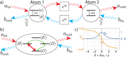
The quantum diode consists of a pair of spatially-separated, nondegenerate atoms in a 1D waveguide, shown in Fig. 1a, tuned to discriminate between a coherent field $\alpha$ incident from the left, and a coherent field $\beta$ incident from the right. Prima facie, this appears to violate reciprocity: the transmission coefficients of a passive, linear, time-reversal-symmetric scatterer should satisfy $\mathcal{T}_{\leftarrow}=\mathcal{T}_{\rightarrow}$, so there is an interesting question as to the origin of the transmission asymmetry.

Refer to caption
Figure 1: (colour online) (a) Schematic illustration of two atoms in a wave-guide, driven by a field incident from the left with amplitude $\left\langle a_{\rm in}\right\rangle=\alpha$, or from the right with $\left\langle b_{\rm in}\right\rangle=\beta$. (b) Hybridised model, in which an incident field scatters strongly (i.e. reflects) off the $\left|G\right\rangle=\left|gg\right\rangle\leftrightarrow\left|B\right\rangle\sim\left|eg\right\rangle-\left|ge\right\rangle$ transition. For a field incident from the left, interference between direct and indirect excitation channels couple weakly to the dark state $\left|D\right\rangle\sim\left|eg\right\rangle+\left|ge\right\rangle$. Driving from the right does not couple to $\left|D\right\rangle$. (c) Reflectance $\mathcal{R}$ and phase shift $\varphi$ versus dimensionless detuning, $\delta=\delta\omega_{1}/\gamma$, for a field reflected off a single atom.

Here, we derive a master equation for the driven two-atom system shown in Fig. 1a. We show that the two-atom dark state Fang and Baranger (2017) responsible for the asymmetry arises from entanglement between the matter and the field Makarov and Letokhov (2003). This leads to non-reciprocal Jalas et al. (2013) and incoherent Fang and Baranger (2017) scattering matrices, and we establish the maximum possible ‘diode efficiency’ Dai et al. (2015) of $2/3$, for which the steady state is inverted. Finally, we show that a toy-model of a randomly fluctuating mirror replicates the statistics of the scattered field and corresponds exactly to the rate equation model when adiabatically eliminating all coherences.

The picture that emerges is that in the steady-state, under cw-driving from one direction, the two atoms become entangled with the local electromagnetic field in a tripartite $\left|W\right\rangle$ state. In the atomic Hilbert space, this corresponds to a long-lived, probabilistic mixture of the ground and dark states. Since scattering arises from coherence between the ground and bright states, the dark state population effectively decouples the scatterer from the field, resulting in non-zero transmission. In contrast, driving from the opposite direction does not couple to the dark state at all. Based on these observations, we argue that the device should be understood as a saturable Yagi-Uda antenna (a directional dipole array) Kosako et al. (2010); Lembessis et al. (2013), and we speculate that non-reciprocity may be enhanced in an $n>2$ atom device.

This paper is organised as follows: We introduce the master equation describing the two atoms and the coherent drive via the waveguides in Section I and then start the analysis in Section II by calculating the steady-state of the two atoms under driving in the parameter regime relevant for rectification. These results then motivate the division of the two atom Hilbert space into a fast and slow subspace and we derive the dynamical equations for the scattering when adiabatically eliminating the fast subspace in the following Section III and discuss the scattering characteristics of this system in Section IV. Another step of adiabatically eliminating the remaining coherences in the slow subspace then leads to a toy model of a “flapping” mirror, which we explore in section V before discussing the rectification properties of this device in Section VI. The appendix containfes details of the calculations and derivations.

I System

We model the system of two two-level atoms depicted in Fig. 1b, bi-directionally cascaded in a 1D waveguide Zeeb et al. (2015); Combes et al. (2017) (also see appendix A). The atoms are driven by a coherent field at frequency $\omega_{c}$, and separated by a distance $d$ (with corresponding phase shift $\phi=\omega_{c}d/c_{s}=2\pi d/\lambda_{c}$ Lalumière et al. (2013)). The device operates near the first resonance, for which the inter-atomic spacing is half a wavelength, i.e. $\phi\approx\pi$. The evolution of the system in the local atomic basis $\{{\left|gg\right\rangle},{\left|ge\right\rangle},{\left|eg\right\rangle},{\left|ee\right\rangle}\}$ is described by Hamiltonian terms and dissipators

$\displaystyle H_{k}=-\omega_{k}\,\sigma_{z}^{(k)}/2\,,\quad L_{k}=\sqrt{{\gamma_{k}}/2}\,\sigma_{-}^{(k)}\,,$ (1)

with $k=1,2$ for the two atoms in the waveguide, and $\sigma_{-}={\left|g\right\rangle}{\left\langle e\right|}$. The master equation for the two-atom density matrix is

$\displaystyle\dot{\rho}=\mathcal{L}\rho\equiv-\mathrm{i}\left[H_{T},\rho\right]+\mathcal{D}[L_{\rightarrow}]\rho+\mathcal{D}[L_{\leftarrow}]\rho,$ (2)

where $\mathcal{D}[X]\rho=X\rho X^{\dagger}-\tfrac{1}{2}(X^{\dagger}X\rho+\rho X^{\dagger}X)$, and

$\displaystyle H_{T}=$ $\displaystyle H_{1}+H_{2}-\mathrm{i}\big{(}\alpha L_{1}^{\dagger}-\alpha^{\ast}L_{1}\big{)}/2-\mathrm{i}\big{(}\beta L_{2}^{\dagger}-\beta^{\ast}L_{2}\big{)}/2$
$\displaystyle-\mathrm{i}\big{(}\mathrm{e}^{\mathrm{i}\phi}L_{2}^{\dagger}(L_{1}+\alpha)-\mathrm{e}^{-\mathrm{i}\phi}(L_{1}^{\dagger}+\alpha^{\ast})L_{2}\big{)}/{2}$
$\displaystyle-\mathrm{i}\big{(}\mathrm{e}^{\mathrm{i}\phi}L_{1}^{\dagger}(L_{2}+\beta)-\mathrm{e}^{-\mathrm{i}\phi}(L_{2}^{\dagger}+\beta^{\ast})L_{1}\big{)}/{2}\,,$ (3)
$\displaystyle L_{\rightarrow}=$ $\displaystyle L_{2}+\mathrm{e}^{\mathrm{i}\phi}L_{1}+\mathrm{e}^{\mathrm{i}\phi}\alpha\,,$ (4)
$\displaystyle L_{\leftarrow}=$ $\displaystyle L_{1}+\mathrm{e}^{\mathrm{i}\phi}L_{2}+\mathrm{e}^{\mathrm{i}\phi}\beta\,.$ (5)

Terms like $L_{2}^{\dagger}L_{1}$ in $H_{T}$ represent effective inter-atomic coupling, induced by their mutual coupling to the waveguide.

The left-moving output field amplitude and photon flux are, respectively

$\displaystyle\alpha_{\text{out}}(t)$ $\displaystyle=\langle a_{\text{out}}(t)\rangle=\text{Tr}\left\{L_{\leftarrow}\rho\right(t)\},$
$\displaystyle\mathcal{A}_{\text{out}}(t)$ $\displaystyle=\langle a_{\text{out}}^{\dagger}a_{\text{out}}(t)\rangle=\text{Tr}\left\{L^{\dagger}_{\leftarrow}L_{\leftarrow}\rho(t)\right\}.$ (6)

The right-moving amplitude, $\beta_{\text{out}}$, and flux, $\mathcal{B}_{\text{out}}$, depend similarly on $L_{\rightarrow}$. Without loss of generality, we consider the two atoms to be coupled symmetrically to the waveguide, so that $\gamma_{1}=\gamma_{2}=\gamma$.

Atom 2 (depicted in Fig. 1) is resonant with the carrier frequency, $\omega_{c}$, and to break inversion symmetry, we detune atom 1 by an amount $\omega_{1}-\omega_{c}=\delta\omega_{1}\equiv-\delta\,\gamma$. In linear response, the reflectance of each atom is a Lorentzian in the dimensionless detuning, $\delta$, as shown in Fig. 1c, and there is a corresponding phase shift, $\varphi$, in transmission. For small detuning, this phase shift is $\varphi\approx-\delta$. We perturb the geometric inter-atomic separation to compensate for this phase shift, so that $\phi=\pi-\delta$. This choice of $\delta\omega_{1}$ and $\phi$ is consistent with Ref. Dai et al. (2015) and, as shown in appendix C, optimises the asymmetry in the response of the system. In what follows, we adopt units where $\gamma=1$.

II Steady state

As we are interested in the scattering properties of the two-atom system, we start our analysis by calculating the steady-state of the atoms under driving from either left or right. The results of this section will guide the subsequent analysis and allow us to identify a reduced slow subspace relevant for the scattering dynamics, and which will enable us to adiabatically eliminate fast degrees of freedom from the cascaded master equation in Section III.

We solve for the steady-state of the master equation, $\mathcal{L}\rho_{ss}^{(\alpha,\beta,\delta)}=0$, perturbatively in $\delta$, using the expansions

$\displaystyle\rho_{ss}^{(\alpha,\beta,\delta)}$ $\displaystyle=$ $\displaystyle\bar{\rho}_{0}+\mathrm{i}\delta\bar{\rho}_{1}+\delta^{2}\bar{\rho}_{2}+\ldots,$
$\displaystyle\mathcal{L}$ $\displaystyle=$ $\displaystyle\mathcal{L}_{0}+\mathrm{i}\delta\mathcal{L}_{1}+\delta^{2}\mathcal{L}_{2}+\ldots.$ (7)

This expansion assumes that $\delta$ is the smallest quantity in the problem, consistent with earlier treatment of this problem Dai et al. (2015); Fang and Baranger (2017). Further, we assume that driving is far below the saturation power for each individual atom, so that $\delta\ll|\alpha|+|\beta|\ll\gamma=1$. This allows us to make analytic progress, and, as we show is the regime in which interesting physics occurs.

The solution to the zeroth-order equation, $0=\mathcal{L}_{0}\bar{\rho}_{0}$ is the nullspace of the superoperator $\mathcal{L}_{0}$, which is two-fold degenerate,

$\displaystyle\bar{\rho}_{0}=p_{G}(\alpha,\beta,\delta)\,\bar{\rho}_{0}^{(1)}+p_{D}(\alpha,\beta,\delta)\,\bar{\rho}_{0}^{(2)}\,,$ (8)

where $\bar{\rho}_{0}^{(1)}={\left|G\right\rangle}{\left\langle G\right|}+O(\alpha^{2},\beta^{2})$ and $\bar{\rho}_{0}^{(2)}={\left|D\right\rangle}{\left\langle D\right|}$, $\left|G\right\rangle={\left|gg\right\rangle}$, $\left|D\right\rangle=(\left|ge\right\rangle+\left|eg\right\rangle)/\sqrt{2}$ is the ‘dark’ state, and $p_{G/D}$ are as-yet undetermined coefficients. As shown in appendix B, the system thus hybridises into the symmetric ($\left|D\right\rangle$) and antisymmetric ($\left|B\right\rangle$) states shown in Fig. 1b, in which the steady state is well-approximated by a probabilisitic mixture of the ground state and the dark state.

We calculate the higher-order corrections, $\bar{\rho}_{j}$, by a generalised nullspace analysis of the higher-order expansions of $\mathcal{L}\bar{\rho}=0$ (see appendix D). At second order we find that $p_{G}$ and $p_{D}$ are related by

$\displaystyle p_{D}/p_{G}=\left\{\begin{array}[]{lc}2+\alpha^{2}+2\alpha^{4}&\textrm{for $\alpha$ driving ($\beta_{\textrm{in}}=0$)}\\ \beta^{2}+2\beta^{4}&\textrm{for $\beta$ driving ($\alpha_{\textrm{in}}=0$)}\end{array}\right..$ (11)

Together with normalisation, $\text{Tr}\{\bar{\rho}_{0}\}=p_{G}+p_{D}=1$, we find

$\displaystyle\rho_{ss}^{(\alpha,0,\delta)}$ $\displaystyle=\tfrac{1}{3}{\left|G\right\rangle}{\left\langle G\right|}+\tfrac{2}{3}{\left|D\right\rangle}{\left\langle D\right|}+O(\alpha^{2}),$
$\displaystyle\rho_{ss}^{(0,\beta,\delta)}$ $\displaystyle={\left|G\right\rangle}{\left\langle G\right|}+O(\beta^{2}).$ (12)

Thus, for $\alpha$-driving (i.e. from the left), the steady-state of the system is dominated by the dark state, whereas $\beta$ driving (i.e. from the right) is decoupled from the dark state, and leaves the atoms in the ground state. These results are apparently independent of the driving amplitudes. For $\alpha$ driving, this arises because the dark state transition becomes saturated at surprisingly low powers.

We make several observations about this result. Firstly, the steady state depends on the driving direction, which accounts for the asymmetric response to driving fields that has been discussed elsewhere. Secondly, the atomic steady state, $\rho_{ss}^{(\alpha)}$, is mixed, but retains some entanglement (with respect to any local atomic basis) between the atoms due to the dark state component: the concurrence of ${\bar{\rho}_{0}}$ is $C_{\bar{\rho}_{0}}=p_{D}^{2}$, so that $C_{\rho_{ss}^{(\alpha)}}\approx 4/9>0$. Lastly, $\rho_{ss}^{(\alpha)}$ exhibits steady-state population inversion, since the ground state population is $p_{G}\approx 1/3<1/2$.

For a symmetric system ($\delta=0$), the dark state is completely decoupled from the field and thus in principle infinitely long-lived. Conversely, for small $|\delta|>0$, the dark state is very weakly coupled to the waveguide, so that it has an anomalously long lifetime. As we show in appendix B, there is a fast time scale associated with the bright state $\left|B\right\rangle=(\left|ge\right\rangle-\left|eg\right\rangle)/\sqrt{2}$, given by $\tau_{B}^{-1}=\gamma_{B}=2\gamma+O(\delta^{2})$, and a slow time scale associated with the dark state, given by $\tau_{D}^{-1}=\gamma_{D}=\delta^{2}\gamma+O(\delta^{3})$ Redchenko and Yudson (2014); Fang and Baranger (2017). It is this slow timescale that leads to a saturation of the ground state to dark state transition at very low incident power.

Finally, the purification Nielsen and Chuang (2000) of $\rho_{ss}^{(\alpha)}$ is the tripartite $\left|W\right\rangle$ state

$$\left|W\right\rangle=(\left|eg0\right\rangle+\left|ge0\right\rangle+\left|gg1\right\rangle)/\sqrt{3},$$

where we have introduced a purifying system labeled by the states $\left|0\right\rangle$ and $\left|1\right\rangle$. In this picture, $\left|0\right\rangle$ corresponds to the incident field being transmitted, and $\left|1\right\rangle$ corresponds to the incident field being reflected Makarov and Letokhov (2003). The evolution of the field-plus-atom is unitary, so that the purifying system has support on the field modes $a_{\rm out}^{\dagger}$ and $b_{\rm out}^{\dagger}$ Makarov and Letokhov (2003); Redchenko and Yudson (2014), corresponding to the ‘recently-scattered’ field. That is, the slow subspace of the atoms is entangled with the field out to a distance $\sim\tau_{D}c_{s}$.

III Adiabatic elimination

In light of the steady-state analysis above and the separation of time-scales discussed there, we adiabatically eliminate the fast subspace spanned by $\mathcal{F}=\{{\left|B\right\rangle},{\left|E\right\rangle}\}$, where $\left|E\right\rangle={{\left|ee\right\rangle}}$, to yield dynamics in the slow subspace, spanned by $\mathcal{S}=\{{\left|G\right\rangle},{\left|D\right\rangle}\}$. We apply the adiabatic elimination procedure from Refs. Bouten and Silberfarb (2008); Bouten et al. (2008); Combes et al. (2017), to get the SLH triple for the system restricted to the slow subspace. As described in appendix E, to lowest non-trivial order in $\alpha,\beta$ and $\delta$ we derive the adiabatically eliminated operators

$\displaystyle\tilde{H}_{T}$ $\displaystyle={\alpha\,\delta\,}\tilde{\sigma}_{x}/2\,,$ (13)
$\displaystyle\tilde{L}_{\rightarrow}$ $\displaystyle=\tfrac{1}{2}\big{(}(\alpha-\beta)\tilde{\sigma}_{z}-(\alpha+\beta)\mathds{1}\big{)}\,,$
$\displaystyle\tilde{L}_{\leftarrow}$ $\displaystyle=\mathrm{i}\,\delta\,\tilde{\sigma}_{-}-\tfrac{1}{2}\big{(}(\alpha-\beta)\tilde{\sigma}_{z}+(\alpha+\beta)\mathds{1}\big{)}\,,$ (14)

where $\tilde{\sigma}_{z}={\left|G\right\rangle}{\left\langle G\right|}-{\left|D\right\rangle}{\left\langle D\right|}$, $\tilde{\sigma}_{x}=\tilde{\sigma}_{-}+\tilde{\sigma}_{+}$, and $\tilde{\sigma}_{-}=\left|G\right\rangle\left\langle D\right|$. We note that this adiabatic elimination does not rely on the earlier perturbative assumption that $\delta\ll\alpha,\beta$, rather it merely requires $\delta,\alpha,\beta\ll\gamma=1$.

The coherent part of the master equation generated by $\tilde{H}_{T}$ accounts for the asymmetry observed in the steady state: the effective Hamiltonian, $\tilde{H}_{T}$, vanishes for $\beta$ driving (i.e. from the right), so that the dynamics within the slow subspace is completely decoupled from $\beta$.

Refer to caption
Figure 2: (colour online) Correlation functions, $g^{(1)}(\tau)$ and $g^{(2)}(\tau)$, for reflection and transmission, under $\alpha$ driving. We can calculate these correlation functions using the full four-dimensional Hilbert space, the adiabatically-eliminated two-dimensional space, and the ‘flapping-mirror’ toy-model. The differences between these calculation methods are $\sim(\delta/\alpha)^{2}=10^{-6}$, so are not visible on this scale.

The effective Lindblad operator $\tilde{L}_{\leftarrow}$ is a coherent combination of dephasing and relaxation. Together with the $\alpha$-dependent driving in $\tilde{H}_{T}$, the system evolves to an inverted steady state: without the interplay between driving and dissipation, the maximum population of the dark state would be bounded by $p_{D}<1/2$ Stace et al. (2005); Hughes and Carmichael (2011, 2013); Stace et al. (2013); Colless et al. (2014).

The steady-state in the slow subspace, $\mathcal{S}$, is then

$\displaystyle\tilde{\rho}_{ss}^{(\alpha,\beta,\delta)}\!=\!\frac{1}{6\alpha^{2}\!+\!2\beta^{2}\!+\!\delta^{2}}\!\left[\begin{array}[]{cc}2\alpha^{2}\!+\!2\beta^{2}\!+\!\delta^{2}&2\mathrm{i}\alpha\delta\!\\ -2\mathrm{i}\alpha\delta&4\alpha^{2}\!\end{array}\right].$ (17)

This result does not require $\delta\ll|\alpha|+|\beta|$ as in Eqs. (11) and (12), however, naturally, it agrees with those results in the limits $\alpha\rightarrow 0$ or $\beta\rightarrow 0$. Together with $\tilde{L}_{\rightleftharpoons}$ in Eq. (14), Eq. (17) enables us to find analytical expressions for the field fluxes.

IV Scattering

Using the adiabatically eliminated operators, we calculate the scattering matrices for field amplitudes, $S$, and fluxes, $T$. Writing

$\displaystyle\left[\begin{array}[]{c}\alpha_{\text{out}}\\ \beta_{\text{out}}\end{array}\right]=S\left[\begin{array}[]{c}\alpha\\ \beta\end{array}\right]\,,\quad\left[\begin{array}[]{c}\mathcal{A}_{\text{out}}\\ \mathcal{B}_{\text{out}}\end{array}\right]\!=T\left[\begin{array}[]{c}{\mathcal{A}_{\text{in}}}\\ {\mathcal{B}_{\text{in}}}\end{array}\right]\,,$ (26)

where ${\mathcal{A}_{\text{in}}}=|\alpha|^{2}$, ${\mathcal{B}_{\text{in}}}=|\beta|^{2}$, we find

$\displaystyle S$ $\displaystyle=-\left[\begin{array}[]{cc}\frac{2\alpha^{2}-\delta^{2}}{6\alpha^{2}+\delta^{2}}&0\\ \frac{4\alpha^{2}}{6\alpha^{2}+\delta^{2}}&1\end{array}\right]\approx-\left[\begin{array}[]{cc}1/3&0\\ 2/3&1\end{array}\right],$ (31)
$\displaystyle T$ $\displaystyle\!=\!\left[\begin{array}[]{cc}\!\!\mathcal{R}_{\alpha}\!&\!\mathcal{T}_{\beta}\!\!\\ \!\!\mathcal{T}_{\alpha}\!&\!\mathcal{R}_{\beta}\!\!\end{array}\right]\!=\!\left[\begin{array}[]{cc}\!p_{G}^{(\alpha,0,\delta)}&\!p_{D}^{(0,\beta,\delta)}\!\\ \!p_{D}^{(\alpha,0,\delta)}\!&\!p_{G}^{(0,\beta,\delta)}\!\end{array}\right]\!\approx\!\left[\begin{array}[]{cc}\!1/3&\!0\!\\ \!2/3&\!1\!\end{array}\right]\!,$ (38)

where $p_{K}^{(\alpha,\beta,\delta)}=\left\langle K\right|\tilde{\rho}_{ss}^{(\alpha,\beta,\delta)}\left|K\right\rangle$, and the approximations hold for $\delta\ll|\alpha|+|\beta|$. Up to an overall sign, the scattering matrices in Eqs. (31) and (38) are identical.

We see that $S\neq S^{T}$, consistent with the definition of an (imperfect) isolator. For this system, the Lorentz reciprocity theorem is broken by the nonlinear saturation of the atoms Jalas et al. (2013).

Further, $S$ is not unitary, indicating that the scattered field is not fully coherent for $\alpha$ driving. One way to see this is to note that for $\alpha\neq 0$ we find $\mathcal{A}_{\text{out}}\neq|\alpha_{\text{out}}|^{2}$, i.e. the output field flux is not equal to the square of the output field amplitude, as it would be for a coherent state. Conversely, for $\beta$ driving, the dark state remains unpopulated, and if $|\beta_{\text{in}}|^{2}\ll\gamma$, the bright state will be unsaturated, so that the atoms will reflect the incident field Peropadre et al. (2013). In this case, the output field is coherent as it is simply the reflected input field.

While these observations imply the field is incoherent, there are many different ways in which incoherence may be manifest. To quantify the incoherent scattering for $\alpha$ driving, we calculate the steady-state output-field correlation functions,

$\displaystyle g_{\text{ref}}^{(1)}(\tau)$ $\displaystyle=$ $\displaystyle\langle a_{\text{out}}^{\dagger}(t+\tau)a_{\text{out}}(t)\rangle/\mathcal{A}_{\text{out}},$
$\displaystyle g^{(2)}_{\text{ref}}(\tau)$ $\displaystyle=$ $\displaystyle\langle a_{\text{out}}^{\dagger}(t)a_{\text{out}}^{\dagger}(t+\tau)a_{\text{out}}(t+\tau)a_{\text{out}}(t)\rangle/\mathcal{A}_{\text{out}}^{2}$

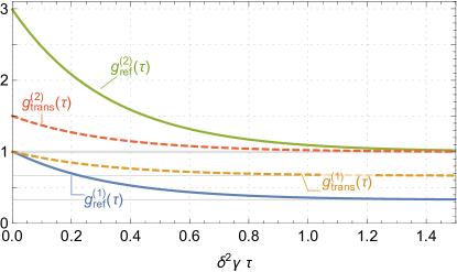
and similar for the transmitted field correlations, $g_{\text{trans}}^{(1,2)}(\tau)$ Fang and Baranger (2017) (see also appendix F). Further, the spectrum of the scattered field can be computed directly from $g^{(2)}_{\text{ref}}(\tau)$, so this may be useful for experimental comparison. We will later compare these correlation functions to the result of a simple “flapping mirror” model, and show that they are essentially indistinguishable.

For $\alpha$ driving (from the dark state coupling direction), the two-time field-field correlations functions, $g^{(1)}(\tau)$, for the reflected and transmitted fields satisfy $g^{(1)}_{\text{ref}}(0)=g^{(1)}_{\text{trans}}(0)=1$, and

$\displaystyle\lim_{\tau\rightarrow\infty}g^{(1)}_{\text{ref}}(\tau)$ $\displaystyle=\frac{(2\alpha^{2}-\delta^{2})^{2}}{(4\alpha^{2}+\delta^{2})^{2}-4\alpha^{4}}=\!\frac{1}{3}+O\Big{(}\frac{\delta^{2}}{\alpha^{2}}\!\Big{)},$
$\displaystyle\lim_{\tau\rightarrow\infty}g^{(1)}_{\text{trans}}(\tau)$ $\displaystyle=\frac{4\alpha^{2}}{6\alpha^{2}+\delta^{2}}=\frac{2}{3}+O\Big{(}\frac{\delta^{2}}{\alpha^{2}}\Big{)}\,.$

The flux-flux correlation function $g^{(2)}$ satisfies $\lim_{\tau\rightarrow\infty}g^{(2)}_{\text{ref}}(\tau)=\lim_{\tau\rightarrow\infty}g^{(1)}_{\text{trans}}(\tau)=1$, and

$\displaystyle g^{(2)}_{\text{ref}}(0)$ $\displaystyle=\frac{6\alpha^{2}+\delta^{2}}{2\alpha^{2}+\delta^{2}}=3+O\Big{(}\frac{\delta^{2}}{\alpha^{2}}\Big{)},$
$\displaystyle g^{(2)}_{\text{trans}}(0)$ $\displaystyle=\frac{3}{2}+\frac{\delta^{2}}{4\alpha^{2}}.$

At long times, $g^{(1)}(\tau)$ is sub-unity, indicating incoherent statistics, while $g^{(2)}(\tau)>1$, indicating thermal or bunched light. At intermediate times, the correlation functions decay exponentially between the above limits, as shown in Fig. 2.

The correlation functions for $\beta$ driving (from the decoupled direction) are unity for all time (up to corrections of order $\delta^{2}/\alpha^{2}$).

The incoherence of the outgoing field under $\alpha$ driving arises from two competing effects: firstly, the drive couples weakly to the dark state, so that when $\delta^{2}\gamma\ll\alpha^{2}\ll\gamma=1$, the dark state becomes ultra-saturated (i.e. inverted) over a time $\sim\tau_{D}$. Secondly, the input field reflects off the strongly coupled dipole transition $\left|G\right\rangle\leftrightarrow\left|B\right\rangle$, so that when the system is shelved in the dark state, $\left|D\right\rangle$, it becomes transparent. At steady-state, the system thus fluctuates between the ground state, which coherently reflects the incoming field as would a single-atom mirror Peropadre et al. (2013); Lu et al. (2014), and the dark state, which is transparent to the driving field. The normalised output flux is thus equal to the dark state probability, $p_{D}=2/3$.

Refer to caption
Figure 3: (colour online) Transmittance versus incident power, $|\alpha_{\text{in}}|^{2}/\gamma$ or $|\beta_{\text{in}}|^{2}/\gamma$. The dark state becomes saturated for $|\alpha|^{2}\gtrsim\delta^{2}$, so that $\mathcal{T}_{\alpha}$ has a dark-state saturation plateau for $\delta^{2}\lesssim|\alpha|^{2}/\gamma\lesssim 1$ wherein $\mathcal{T}_{\alpha}\approx 2/3=p_{D}$. $\mathcal{T}_{\beta}$ is independent of $\delta$. The bright state also becomes saturated when $|\alpha|^{2},|\beta|^{2}\gtrsim\gamma$, so that $\mathcal{T}_{\alpha}$ and $\mathcal{T}_{\beta}$ both asymptote to unity when $|\alpha|^{2},|\beta|^{2}\gtrsim\gamma$. Solid curves are calculated using the full four-dimensional Hilbert space. Dashed curves are calculated for the two-dimensional slow subspace (adiabatically elimination) which are valid for $|\alpha|^{2},|\beta|^{2}\ll\gamma$, and are plotted with a small offset for visibility. Also shown is the ‘diode efficiency’ $\mathcal{E}$ (dotted) for $\delta=10^{-3}$, as defined in Dai et al. (2015).

V Poisson Rate Equations and Flapping Mirror Model

The correlation functions can be understood from a simple rate model in which we eliminate the off-diagonal elements $\rho_{DG}$ and $\rho_{GD}$ in Eq. (1), assuming the reduced Hamiltonian and Lindblad operators given in Eq. (14). As described in Appendix G, for $\alpha$-driving, we find

$\displaystyle\left[\begin{array}[]{c}\dot{P}_{D}\\ \dot{P}_{G}\end{array}\right]$ $\displaystyle\approx\left[\begin{array}[]{cc}-\delta^{2}&\hphantom{-}2\delta^{2}\\ \hphantom{-}\delta^{2}&-2\delta^{2}\\ \end{array}\right]\left[\begin{array}[]{c}P_{D}\\ P_{G}\end{array}\right].$ (45)

Since the dark state, $\left|D\right\rangle$, is transparent to the incident field (so the reflectivity of the system is $R=0$), and the ground state $\left|G\right\rangle$ reflects the field (so the reflectivity is $R=1$), this expression motivates a simple “flapping-mirror” classical rate model, which replicates the output field correlation functions.

Suppose a black-box optical-circuit consists of a mirror which flips in and out of the optical path, controlled by a two-state random variable $R\in\{0,1\}\leftrightarrow\{D,G\}$, where the arrow indicates a precise correspondence between the notional reflectivity of the mirror, and the state of the two-atom system in the reduced slow subspace. For $R=1$, the optical circuit is fully reflective (i.e. reflectance $\mathcal{R}_{1}=1$), and when $R=0$ the circuit is fully transparent, (i.e. reflectance $\mathcal{R}_{0}=0$). We assume the black box responds asymmetrically to light incident from different directions 111Such a scheme is physically realisable by using a QND detection of photon flux to determine from which direction the field is incident, and controlling the mirror accordingly: for light incident from the right, we fix $R=1$ so that $\mathcal{R}_{1}=1$; for light incident from the left we drive the state of the mirror with a Poisson process following a simple two-state rate model with transition rates $\Gamma_{R\overline{R}}$, from state $R$ to $\overline{R}$, given by the matrix elements in Eq. (45). Starting in state $R$, the flapping mirror will be found in that state after time $\tau$ with probability

$$P_{R,R}(\tau)=p_{R}-(1-p_{R})e^{-\Gamma_{\text{tot}}t}$$ (46)

where $p_{0}=p_{D}=2/3$ and $p_{1}=p_{G}=1/3$ are the steady-state probabilities of state $R$, i.e. $p_{R}=\Gamma_{\overline{R}R}/\Gamma_{\text{tot}}$, $\Gamma_{01}=\Gamma_{D}=\delta^{2}\gamma=\Gamma_{10}/2$, and $\Gamma_{\text{tot}}=\Gamma_{01}+\Gamma_{10}=3\delta^{2}\gamma$.

In appendix H we discuss in detail the statistics of a coherent state of amplitude $\alpha_{\text{in}}$ passing through this flapping mirror device. The reflected and transmitted field amplitudes are $\{\alpha_{\text{out}},\beta_{\text{out}}\}=\{p_{1}\alpha,p_{0}\alpha\}$, the fluxes are $\{\mathcal{A}_{\text{out}},\mathcal{B}_{\text{out}}\}=\{p_{1}|\alpha|^{2},p_{0}|\alpha|^{2}\}$, and the correlation functions are

$\displaystyle g_{\text{ref}}^{(1)}(\tau)$ $\displaystyle=$ $\displaystyle P_{1,1}(\tau),$ (47)
$\displaystyle g_{\text{trans}}^{(1)}(\tau)$ $\displaystyle=$ $\displaystyle P_{0,0}(\tau),$ (48)
$\displaystyle g_{\text{ref}}^{(2)}(\tau)$ $\displaystyle=$ $\displaystyle P_{1,1}(\tau)/p_{1},$ (49)
$\displaystyle g_{\text{trans}}^{(2)}(\tau)$ $\displaystyle=$ $\displaystyle P_{0,0}(\tau)/p_{0}.$ (50)

We see that the output field amplitudes and fluxes of the flapping mirror model agree with the two-atom scattering results in Eqs. (31) and (38) (up to overall phase). The correlation functions of the flapping mirror model completely replicate the corresponding correlation functions of the $\alpha$-driven, two-atom system, and are visually indistinguishable from the traces plotted in Fig. 2.

VI Rectification

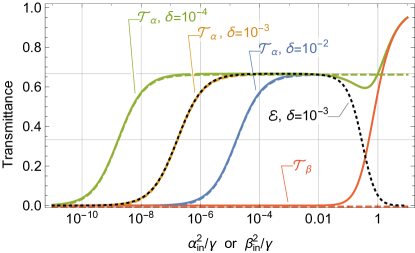
The asymmetry of the flux through the device has attracted some interest due to an analogy with a diode: the system appears to ‘rectify’ flux from one side. This is manifest in the transmission coefficients, in Fig. 3, which shows $\mathcal{T}_{\alpha}$ for several different values of $\delta$, and $\mathcal{T}_{\beta}$, which is essentially independent of $\delta$. There is a clear plateau where $\mathcal{T}_{\alpha}\approx 2/3$, for $\delta^{2}\gamma\ll\alpha_{\text{in}}\ll\gamma=1$. This is consistent with the flux scattering matrix elements in Eq. (38), which shows that the transmission coefficient, $\mathcal{T}_{K}$ is just the dark state probability. The low-power roll-off of $\mathcal{T}_{\alpha}$ corresponds to the saturation intensity of the dark state, which is small due to the extremely weak dark-state coupling at small $\delta$.

Previous work has quantified this asymmetry using the ‘diode efficiency’ Dai et al. (2015), defined as

$$\mathcal{E}=\mathcal{T}_{\alpha}(\mathcal{T}_{\alpha}-\mathcal{T}_{\beta})/(\mathcal{T}_{\alpha}+\mathcal{T}_{\beta}).$$

Clearly, in the regime where the asymmetry is greatest, $\mathcal{T}_{\beta}\ll\mathcal{T}_{\alpha}$, so that $\mathcal{E}\approx\mathcal{T}_{\alpha}=p_{D}(\alpha,0,\delta)$. The diode efficiency $\mathcal{E}$ is shown as a dotted curve in Fig. 3, and tracks $\mathcal{T}_{\alpha}$ until the bright state starts to become saturated at high power. As discussed in appendix C we numerically optimise $\mathcal{E}$ over $\delta\phi$ and $\delta\omega$, and we find the maximum value, $\mathcal{E}=p_{D}\approx 2/3$, at the settings $\delta\phi=-\delta\omega=\delta$ that we have adopted throughout.

Refer to caption
Figure 4: (colour online) Radiated flux from the dark state, $\left|D\right\rangle$, moving left, $\mathcal{A}_{\text{out}}$, and right, $\mathcal{B}_{\text{out}}$, showing strong asymmetry in the emission profile, analogous to a Yagi-Uda directional transmitter. The main panel shows flux over long time-scales $\gamma t\sim\delta^{-2}\gg 1$; inset shows flux over short time-scales, $\gamma t\sim 1$.

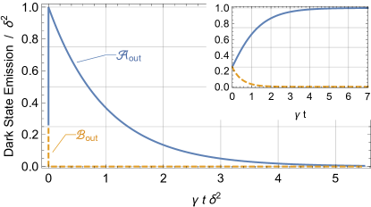
The underlying asymmetry in absorption is manifest from the asymmetric field coupling in the effective Hamiltonian, Eq. (13), and this also gives rise to asymmetric emission from atomic excited states. Fig. 4 shows the time-dependent, left-going flux, $\mathcal{A}_{\textrm{out}}$, and right-going flux, $\mathcal{B}_{\textrm{out}}$, from the dark state Makarov and Letokhov (2003). It is evident that the dark state emits asymmetrically, with the vast majority of energy radiating to the left over a long time $\gamma t\sim\delta^{-2}$. This asymmetric emission is reminiscent of a two-element Yagi-Uda antenna (of the kind used for directional radio transceivers), in which detuned dipole elements behave as ‘reflectors’ and ‘directors’ to produce a directional radiation pattern Kosako et al. (2010); Lembessis et al. (2013).

For $n=2$ atoms, the peak “diode efficiency” $\mathcal{E}=2/3=n/(n+1)$ is equal to the dark state population in the entangled tripartite $\left|W\right\rangle$ state of the atoms and field. By analogy, we speculate that if $n>2$ atoms are suitably tuned (e.g. as in Refs. Stannigel et al. (2012); Ramos et al. (2014); Pichler et al. (2015)), then the diode efficiency $\mathcal{E}$ could be improved for larger $n$, albeit with a narrow bandwidth.

VII Conclusions

To conclude, we have analysed a two-atom system in a 1D waveguide. Consistent with previous results, we find that this system responds asymmetrically to external driving fields when one of the atoms is detuned from the driving field and their separation is close to a half-integer multiple of the wavelength, and we establish the regime where the response is maximally asymmetric.

In addition, we have shown that the onset time for the asymmetry is not instantaneous. Rather, it is established over a time scale set by the dark-state lifetime, which sets a modulation bandwidth for any time-varing signals. The asymmetry in the field coupling leads to an inverted, entangled mixture of the ground and dark states, which is ultimately responsible for nonreciprocal scattering. The scattered field statistics are replicated by a simple stochastic flapping-mirror model, which physically corresponds to fluctuations between the dark and ground states of the atoms.

Acknowledgements.
We thank M. Pletyukhov and P. Rabl for stimulating discussions. This work was supported by the Australian Research Council under the Discovery and Centre of Excellence funding schemes (project numbers DP150101033, DE160100356, and CE110001013).

References

  • Fratini et al. (2014) F. Fratini, E. Mascarenhas, L. Safari, J.-P. Poizat, D. Valente, A. Auffèves, D. Gerace,  and M. F. Santos, “Fabry-perot interferometer with quantum mirrors: Nonlinear light transport and rectification,” Phys. Rev. Lett. 113, 243601 (2014).
  • Dai et al. (2015) J. Dai, A. Roulet, H. N. Le,  and V. Scarani, “Rectification of light in the quantum regime,” Phys. Rev. A 92, 063848 (2015).
  • Mascarenhas et al. (2016) E. Mascarenhas, M. F. Santos, A. Auffèves,  and D. Gerace, “Quantum rectifier in a one-dimensional photonic channel,” Phys. Rev. A 93, 043821 (2016).
  • Fratini and Ghobadi (2016) F. Fratini and R. Ghobadi, “Full quantum treatment of a light diode,” Physical Review A 93, 023818 (2016).
  • Gonzalez-Ballestero et al. (2016) C. Gonzalez-Ballestero, E. Moreno, F. J. Garcia-Vidal,  and A. Gonzalez-Tudela, “Nonreciprocal few-photon routing schemes based on chiral waveguide-emitter couplings,” Phys. Rev. A 94, 063817 (2016).
  • Ordonez-Miranda et al. (2017) J. Ordonez-Miranda, Y. Ezzahri,  and K. Joulain, “Quantum thermal diode based on two interacting spinlike systems under different excitations,” Phys. Rev. E 95, 022128 (2017).
  • Fang and Baranger (2017) Y.-L. L. Fang and H. U. Baranger, “Cascaded emitters in a waveguide: Non-reciprocity and correlated photons at perfect elastic transmission,” Physical Review A 96 (2017).
  • Rudolph et al. (1995) T. G. Rudolph, Z. Ficek,  and B. J. Dalton, “Two-atom resonance fluorescence in running- and standing-wave laser fields,” Phys. Rev. A 52, 636 (1995).
  • Rudolph and Ficek (1998) T. Rudolph and Z. Ficek, “Interference pattern with a dark center from two atoms driven by a coherent laser field,” Phys. Rev. A 58, 748 (1998).
  • Makarov and Letokhov (2003) A. A. Makarov and V. S. Letokhov, “Spontaneous decay in a system of two spatially spearated atoms (one-dimensional case),” Journal of Experimental and Theoretical Physics 97, 688 (2003).
  • Lembessis et al. (2013) V. E. Lembessis, A. A. Rsheed, O. M. Aldossary,  and Z. Ficek, “Two-atom system as a nanoantenna for mode switching and light routing,” Phys. Rev. A 88, 053814 (2013).
  • Laakso and Pletyukhov (2014) M. Laakso and M. Pletyukhov, “Scattering of two photons from two distant qubits: Exact solution,” Phys. Rev. Lett. 113, 183601 (2014).
  • Jalas et al. (2013) D. Jalas, A. Petrov, M. Eich, W. Freude, S. Fan, Z. Yu, R. Baets, M. Popovic, A. Melloni, J. D. Joannopoulos, M. Vanwolleghem, C. R. Doerr,  and H. Renner, “What is — and what is not — an optical isolator,” Nature Photonics 7, 579 (2013).
  • Kosako et al. (2010) T. Kosako, Y. Kadoya,  and H. F. Hofmann, “Directional control of light by a nano-optical yagi-uda antenna,” Nature Photonics 4, 312 (2010).
  • Zeeb et al. (2015) S. Zeeb, C. Noh, A. S. Parkins,  and H. J. Carmichael, “Superradiant decay and dipole-dipole interaction of distant atoms in a two-way cascaded cavity QED system,” Physical Review A 91, 023829 (2015).
  • Combes et al. (2017) J. Combes, J. Kerckhoff,  and M. Sarovar, “The SLH framework for modeling quantum input-output networks,” Advances in Physics: X 2, 784 (2017).
  • Lalumière et al. (2013) K. Lalumière, B. C. Sanders, A. F. van Loo, A. Fedorov, A. Wallraff,  and A. Blais, “Input-output theory for waveguide QED with an ensemble of inhomogeneous atoms,” Phys. Rev. A 88, 043806 (2013).
  • Redchenko and Yudson (2014) E. S. Redchenko and V. I. Yudson, “Decay of metastable states of two qubits in a waveguide,” Physical Review A 90, 063829 (2014).
  • Nielsen and Chuang (2000) M. Nielsen and I. Chuang, Quantum Computation and Quantum Information (Cambridge University Press, 2000).
  • Bouten and Silberfarb (2008) L. Bouten and A. Silberfarb, “Adiabatic elimination in quantum stochastic models,” Communications in Mathematical Physics 283, 491 (2008).
  • Bouten et al. (2008) L. Bouten, R. van Handel,  and A. Silberfarb, “Approximation and limit theorems for quantum stochastic models with unbounded coefficients,” Journal of Functional Analysis 254, 3123 (2008).
  • Stace et al. (2005) T. M. Stace, A. C. Doherty,  and S. D. Barrett, “Population inversion of a driven two-level system in a structureless bath,” Physical Review Letters 95, 106801 (2005).
  • Hughes and Carmichael (2011) S. Hughes and H. J. Carmichael, “Stationary Inversion of a Two Level System Coupled to an Off-Resonant Cavity with Strong Dissipation,” Physical Review Letters 107, 193601 (2011).
  • Hughes and Carmichael (2013) S. Hughes and H. J. Carmichael, “Phonon-mediated population inversion in a semiconductor quantum-dot cavity system,” New Journal of Physics 15, 053039 (2013).
  • Stace et al. (2013) T. M. Stace, A. C. Doherty,  and D. J. Reilly, “Dynamical steady states in driven quantum systems,” Phys. Rev. Lett. 111, 180602 (2013).
  • Colless et al. (2014) J. I. Colless, X. G. Croot, T. M. Stace, A. C. Doherty, S. D. Barrett, H. Lu, A. C. Gossard,  and D. J. Reilly, “Raman phonon emission in a driven double quantum dot,” Nature Communications 5, 3716 EP (2014).
  • Peropadre et al. (2013) B. Peropadre, J. Lindkvist, I.-C. Hoi, C. M. Wilson, J. J. Garcia-Ripoll, P. Delsing,  and G. Johansson, “Scattering of coherent states on a single artificial atom,” New Journal of Physics 15, 035009 (2013).
  • Lu et al. (2014) J. Lu, L. Zhou, L.-M. Kuang,  and F. Nori, “Single-photon router: Coherent control of multichannel scattering for single photons with quantum interferences,” Phys. Rev. A 89, 013805 (2014).
  • Note (1) Such a scheme is physically realisable by using a QND detection of photon flux to determine from which direction the field is incident, and controlling the mirror accordingly.
  • Stannigel et al. (2012) K. Stannigel, P. Rabl,  and P. Zoller, “Driven-dissipative preparation of entangled states in cascaded quantum-optical networks,” New Journal of Physics 14, 063014 (2012).
  • Ramos et al. (2014) T. Ramos, H. Pichler, A. J. Daley,  and P. Zoller, “Quantum spin dimers from chiral dissipation in cold-atom chains,” Phys. Rev. Lett. 113, 237203 (2014).
  • Pichler et al. (2015) H. Pichler, T. Ramos, A. J. Daley,  and P. Zoller, “Quantum optics of chiral spin networks,” Phys. Rev. A 91, 042116 (2015).
  • Gardiner and Zoller (2000) C. W. Gardiner and P. Zoller, Quantum Noise, 2nd ed. (Springer, 2000).

Appendix A SLH modeling

We start from the SLH triple in Eq. (1) for each atomic systems, which are cascaded with two coherent state source models Combes et al. (2017), leading to Equations (3)–(5) in the main text. (See also Eq. (132) and Eqs. (174) - (176) of Combes et al. (2017), for additional discussion).

We may re-factor the SLH master equation to obtain a more accessible form of the operators

$\displaystyle\dot{\rho}=$ $\displaystyle\mathcal{L}\rho=-\mathrm{i}\left[H,\rho\right]+\mathcal{D}[\bar{L}_{1}]\rho+\mathcal{D}[\bar{L}_{2}]\rho\,,$ (51)
$\displaystyle H=$ $\displaystyle H_{0}+H_{C}+H_{D}\,,$ (52)

with the operators

$\displaystyle H_{0}=$ $\displaystyle H_{1}+H_{2}\,,$ (53)
$\displaystyle H_{C}=$ $\displaystyle\frac{1}{2}\sqrt{\gamma_{1}\gamma_{2}}\sin{\phi}\left(\sigma_{-}^{(1)}\sigma_{+}^{(2)}+\sigma_{+}^{(1)}\sigma_{-}^{(2)}\right)\,,$ (54)
$\displaystyle H_{D}=$ $\displaystyle\mathrm{i}\sqrt{\frac{\gamma_{1}}{2}}\big{(}(\alpha^{\ast}+\mathrm{e}^{-\mathrm{i}\phi}\beta^{\ast})\sigma_{-}^{(1)}-(\alpha+\mathrm{e}^{\mathrm{i}\phi}\beta)\sigma_{+}^{(1)}\big{)}$
$\displaystyle+$ $\displaystyle\mathrm{i}\sqrt{\frac{\gamma_{2}}{2}}\big{(}(\beta^{\ast}+\mathrm{e}^{-\mathrm{i}\phi}\alpha^{\ast})\sigma_{-}^{(2)}-(\beta+\mathrm{e}^{\mathrm{i}\phi}\alpha)\sigma_{+}^{(2)}\big{)}\,,$ (55)
$\displaystyle\bar{L}_{1}=$ $\displaystyle L_{1}+\mathrm{e}^{\mathrm{i}\phi}L_{2}\,,$ (56)
$\displaystyle\bar{L}_{2}=$ $\displaystyle L_{2}+\mathrm{e}^{\mathrm{i}\phi}L_{1}\,,$ (57)

where $H_{C}$ describes coupling between the two atoms, mediated by the field and $H_{D}$ is the coherent drive acting on each atom. The modified Lindblad operators $\bar{L}_{1/2}$ now describe purely the decay of the atoms into the field. Note that in order to correctly calculate output field amplitudes and fluxes, we still need to keep in mind the original Lindblad operators, Eqs. (4)-(5). However, the above description correctly reproduces the dynamics of the atomic degrees of freedom, i.e. the master equations is equivalent to Eq. (2).

Appendix B Hamiltonian in dark / bright state basis

Defining the bright and dark states as the symmetric and antisymmetric superposition of the states with a single atomic excitation

$\displaystyle\left|B\right\rangle$ $\displaystyle=\frac{1}{\sqrt{2}}\left(\left|ge\right\rangle-\left|eg\right\rangle\right)\quad,\quad\left|D\right\rangle=\frac{1}{\sqrt{2}}\left(\left|ge\right\rangle+\left|eg\right\rangle\right)\,,$ (58)

we can define new ladder operators as

$\displaystyle\sigma_{-}^{(B)}$ $\displaystyle=\frac{1}{\sqrt{2}}\left(\sigma_{-}^{(2)}-\sigma_{-}^{(1)}\right)\quad,\quad\sigma_{-}^{(D)}=\frac{1}{\sqrt{2}}\left(\sigma_{-}^{(2)}+\sigma_{-}^{(1)}\right)\,,$ (59)

with $\sigma_{+}^{(B)}\left|gg\right\rangle=\left|B\right\rangle$ and $\sigma_{+}^{(D)}\left|gg\right\rangle=\left|D\right\rangle$. In the basis $\left\{\left|gg\right\rangle,\left|D\right\rangle,\left|B\right\rangle,\left|ee\right\rangle\right\}$, we can then write the Hamiltonian of the atoms and their effective coupling as

$\displaystyle H_{0}+H_{C}$ $\displaystyle\approx\frac{1}{2}\left(\begin{array}[]{cccc}-\omega_{1}-\omega_{2}&0&0&0\\ 0&-g_{0}\sin{\phi}&\omega_{2}-\omega_{1}&0\\ 0&\omega_{2}-\omega_{1}&g_{0}\sin\phi&0\\ 0&0&0&\omega_{1}+\omega_{2}\end{array}\right)\,,$ (64)

where $g_{0}=\sqrt{\gamma_{1}\gamma_{2}}$. This expression makes evident that in the dark / bright state basis, a detuning between the two atoms, $\delta\omega=\omega_{1}-\omega_{2}\neq 0$, leads to an effective coupling between the symmetric and the antisymmetric state. Conversely, a coupling term between the atoms will lead to a splitting between the dark and bright state. Assuming equal coupling of the two atoms to the waveguide, $\gamma_{1}=\gamma_{2}=\gamma$, we find for the driving terms and dissipative operators

$\displaystyle H_{D}$ $\displaystyle=-\mathrm{i}\frac{\sqrt{\gamma}}{2}\Bigl{\{}\sigma_{+}^{(D)}(\alpha+\beta)(1+\mathrm{e}^{\mathrm{i}\phi})$
$\displaystyle\quad\quad\quad\quad-\sigma_{+}^{(B)}(\alpha-\beta)(1-\mathrm{e}^{\mathrm{i}\phi})\Bigr{\}}+\text{h.c.},$ (65)
$\displaystyle\bar{L}_{1}$ $\displaystyle=\frac{\sqrt{\gamma}}{2}\Bigl{\{}\sigma_{-}^{(D)}(1+\mathrm{e}^{\mathrm{i}\phi})-\sigma_{-}^{(B)}(1-\mathrm{e}^{\mathrm{i}\phi})\Bigr{\}}\,,$
$\displaystyle\bar{L}_{2}$ $\displaystyle=\frac{\sqrt{\gamma}}{2}\Bigl{\{}\sigma_{-}^{(D)}(1+\mathrm{e}^{\mathrm{i}\phi})+\sigma_{-}^{(B)}(1-\mathrm{e}^{\mathrm{i}\phi})\Bigr{\}}\,.$ (66)

As discussed bellow and in the main text, in the following we adopt optimal parameters $\omega_{1}=-\delta\,\gamma$, $\omega_{2}=0$ and $\phi=\pi-\delta$, with $\delta\ll\gamma=1$, and we will only write the results to lowest non-trivial order in $\delta$.

Then we find for the Hamiltonian of the atoms plus their coupling

$\displaystyle H_{0}+H_{C}$ $\displaystyle\approx\frac{1}{2}\gamma\left(\begin{array}[]{cccc}\delta&0&0&0\\ 0&\delta&\delta&0\\ 0&\delta&-\delta&0\\ 0&0&0&-\delta\end{array}\right).$ (71)

Defining the small parameter $\epsilon=\frac{1}{2}\mathrm{i}\delta$, we can write the driving Hamiltonian as

$\displaystyle H_{D}\approx$ $\displaystyle\phantom{-}\mathrm{i}\sqrt{\gamma}\alpha\Bigl{\{}\left(1-\epsilon\right)\sigma_{+}^{(B)}-\epsilon\sigma_{+}^{(D)}\Bigr{\}}$
$\displaystyle-\mathrm{i}\sqrt{\gamma}\beta\Bigl{\{}\left(1-\epsilon\right)\sigma_{+}^{(B)}+\epsilon\sigma_{+}^{(D)}\Bigr{\}}+\text{h.c.},$ (72)

while for the sum of the two dissipators we find

$\displaystyle\mathcal{D}[\bar{L}_{1}]\rho$ $\displaystyle+\mathcal{D}[\bar{L}_{2}]\rho$
$\displaystyle=2\gamma\left|1-\epsilon\right|^{2}\mathcal{D}[\sigma_{-}^{(B)}]\rho+2\gamma\left|\epsilon\right|^{2}\mathcal{D}[\sigma_{-}^{(D)}]\rho\,.$ (73)

To second order in $\delta$ we thus find the decay rates of the bright and dark states

$\displaystyle\gamma_{B}$ $\displaystyle=2\left|1-\epsilon\right|^{2}\gamma\approx 2\gamma\,,$
$\displaystyle\gamma_{D}$ $\displaystyle=2\left|\epsilon\right|^{2}\gamma\approx{\delta^{2}\gamma}/{2}.$ (74)

Thus the antisymmetric state has a fast decay rate, so that can be identified as the bright state, and the symmetric state has a slow decay rate, making it the dark state.

Appendix C Optimised efficiency

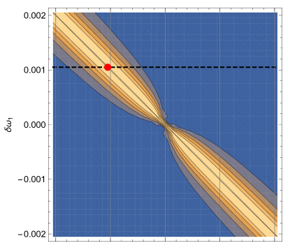
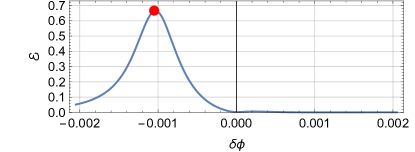
Throughout the preceding analysis, we considered $\delta\phi=-\delta\omega_{1}\equiv\delta$, and $\delta\omega_{2}=0$. This choice of parameters optimises the ‘diode efficiency’ $\mathcal{E}=\mathcal{T}_{\alpha}(\mathcal{T}_{\alpha}-\mathcal{T}_{\beta})/(\mathcal{T}_{\alpha}+\mathcal{T}_{\beta})$, which is a measure of the left-right asymmetry in the flux transmission. To demonstrate this, we numerically tabulate $\mathcal{E}$ over atomic detunings, $\delta\omega_{1}$ and $\delta\omega_{2}$ for each value of $\delta\phi$ . We find the optimal left-right asymmetry when $\delta\omega_{2}=0$, and $\delta\phi=-\delta\omega_{1}\equiv\delta$. Part of this numerical calculation is shown in Fig. 5 in which we fix $\delta\omega_{2}=0$, and find that $\mathcal{E}_{\text{max}}\approx 2/3$ along the optimal parameter choices above. The following analytical calculations, which adopt this parameter choice, confirm this as the maximum diode efficiency.

Refer to caption
Refer to caption
Figure 5: (colour online) (Top) Contour plot of the ‘diode efficiency’, $\mathcal{E}$ as a function of inter-atom path length $\delta\phi$, and the detuning of one atom $\delta\omega_{1}$, assuming $\delta\omega_{2}=0$. (Bottom) Line cut through contour plot along dashed line. The peak efficiency, $\mathcal{E}=2/3$ occurs along the line $\delta\phi=-\delta\omega_{1}\equiv\delta$. Allowing $\delta\omega_{2}$ to vary does not yield a higher value for $\mathcal{E}$.

Appendix D Analytics along optimal parameters

We solve for the steady-state of the master equation, $\mathcal{L}\rho_{ss}=0$, perturbatively in $\delta$, using the expansion

$\displaystyle\rho_{ss}$ $\displaystyle=\bar{\rho}_{0}+\mathrm{i}\delta\bar{\rho}_{1}+\delta^{2}\bar{\rho}_{2}+\ldots$
$\displaystyle\mathcal{L}$ $\displaystyle=\mathcal{L}_{0}+\mathrm{i}\delta\mathcal{L}_{1}+\delta^{2}\mathcal{L}_{2}+\ldots,$ (75)

requiring that the steady-state equation, $\mathcal{L}\rho_{ss}=0$ is fullfilled at all orders of $\delta$ independently. This then leads to a hierarchy of equations for the components of the steady-state density matrix

$\displaystyle 0$ $\displaystyle=\mathcal{L}_{0}\bar{\rho}_{0}$
$\displaystyle 0$ $\displaystyle=\mathcal{L}_{0}\bar{\rho}_{1}+\mathcal{L}_{1}\bar{\rho}_{0}$
$\displaystyle 0$ $\displaystyle=\mathcal{L}_{0}\bar{\rho}_{2}-\mathcal{L}_{1}\bar{\rho}_{1}+\mathcal{L}_{2}\bar{\rho}_{0}$
$\displaystyle\ldots$ (76)

Technically we always solve for the nullspace of a linear system of equations. We find that the nullspace of $\mathcal{L}_{0}$ is two-fold degenerate, so that we can write

$\displaystyle\bar{\rho}_{0}=a_{1}\bar{\rho}_{0}^{(1)}+a_{2}\bar{\rho}_{0}^{(2)}\,,$ (77)

where we leave the coefficients $a_{i}$ arbitrary for the moment. We could fix one of the two coefficients by e.g. requiring the unit trace condition for a valid physical density matrix, but we will only do that later for clarity. The second parameter remains always undetermined at lowest oder $\delta$.

Plugging the zero-th order solution into the first order equation above, Eq. (76), we find a four-fold degenerate nullspace of the first order equations. Two of the solutions correspond to the choice $a_{1}=a_{2}=0$ for $\bar{\rho}_{0}$, in which case the first order equation reduces to finding the nullspace of $\mathcal{L}_{0}$ again.

The other two solutions are non-trivial and together this leads again to a parametrization of the first-order steady-state as

$\displaystyle\bar{\rho}_{1}=b_{1}\bar{\rho}_{1}^{(1)}+b_{2}\bar{\rho}_{1}^{(2)}+b_{3}\bar{\rho}_{0}^{(1)}+b_{4}\bar{\rho}_{0}^{(2)}\,,$ (78)

where the coefficients are initially completely free. Fixing the trace at first order as $\text{Tr}\bar{\rho}_{1}=0$ (to guarantee a valid density matrix for all $\delta$), allows us to fix one of the four parameters in $\bar{\rho}_{1}$. Two of the remaining three parameters can be determined by requiring that the above ansatz actually is a steady-state solution of the master equation to first order in $\delta$, i.e.

$\displaystyle\left(\mathcal{L}_{0}+\mathrm{i}\delta\mathcal{L}_{1}\right)\left(\bar{\rho}_{0}+\mathrm{i}\delta\bar{\rho}_{1}\right)=0$ (79)

to first order in $\delta$. At this point we are thus left with the free parameters $a_{1},a_{2}$ and one of the $b_{i}$, where one of the $a_{i}$ can be determined from the unit trace condition.

Repeating the procedure for the second order equation in the above hierarchy, Eq. (76), then finally allows us to uniquely determine the $a_{i}$. We find

$\displaystyle a_{2}^{(\alpha)}=\frac{1}{2\alpha^{4}}\left(2+\alpha^{2}+2\alpha^{4}\right)a_{1}\quad,\quad a_{2}^{(\beta)}=\left(1+\frac{1}{2\beta^{2}}\right)a_{1}\,,$ (80)

with $a_{1}$ fixed by the trace.

Going to third order in the above hierarchy then uniquely fixes all parameters of the first order parametrisation, and we can write

$\displaystyle\rho_{ss}\approx\bar{\rho}_{0}+\mathrm{i}\delta\bar{\rho}_{1}$ (81)

which is different for driving from either side and coincides well with the numerical solutions for these parameters. For driving from the left, $\beta=0$, we have

$\displaystyle\bar{\rho}_{0}^{(\alpha)}$ $\displaystyle=\frac{1}{a_{0}}\left(\begin{array}[]{cccc}2+2\alpha^{2}+2\alpha^{4}&\sqrt{2}\alpha(1+\alpha^{2})&-\sqrt{2}\alpha(1+\alpha^{2})&-2\alpha^{2}\\ \sqrt{2}\alpha(1+\alpha^{2})&2+\alpha^{2}+2\alpha^{4}&2-\alpha^{2}&-\sqrt{2}\alpha^{3}\\ -\sqrt{2}\alpha(1+\alpha^{2})&2-\alpha^{2}&2+\alpha^{2}+2\alpha^{4}&\sqrt{2}\alpha^{3}\\ -2\alpha^{2}&-\sqrt{2}\alpha^{3}&\sqrt{2}\alpha^{3}&2\alpha^{4}\\ \end{array}\right)\,,$ (86)
$\displaystyle\bar{\rho}_{1}^{(\alpha)}$ $\displaystyle=\frac{1}{a_{0}}\left(\begin{array}[]{cccc}0&\frac{\sqrt{2}}{\alpha}(1+\alpha^{4})&\frac{\sqrt{2}}{\alpha}(1+\alpha^{2}+2\alpha^{4})&2\alpha^{2}\\ -\frac{\sqrt{2}}{\alpha}(1+\alpha^{4})&0&\alpha^{2}&\sqrt{2}\alpha(1+2\alpha^{2})\\ -\frac{\sqrt{2}}{\alpha}(1+\alpha^{4})&-\alpha^{2}&0&\sqrt{2}\alpha(1+2\alpha^{2})\\ -2\alpha^{2}&-\sqrt{2}\alpha(1+2\alpha^{2})&-\sqrt{2}\alpha(1+2\alpha^{2})&0\\ \end{array}\right)\,,$ (91)

with $a_{0}=6+4\alpha^{2}+8\alpha^{4}$. For driving from the right ($\alpha=0$), we find

$\displaystyle\bar{\rho}_{0}^{(\beta)}$ $\displaystyle=\frac{1}{b_{0}}\left(\begin{array}[]{cccc}2(1+\beta^{2}+\beta^{4})&-\sqrt{2}\beta(1+\beta^{2})&\sqrt{2}\beta(1+\beta^{2})&-2\beta^{2}\\ -\sqrt{2}\beta(1+\beta^{2})&\beta^{2}+2\beta^{4}&-\beta^{2}&\sqrt{2}\beta^{3}\\ \sqrt{2}\beta(1+\beta^{2})&-\beta^{2}&\beta^{2}+2\beta^{4}&-\sqrt{2}\beta^{3}\\ -2\beta^{2}&\sqrt{2}\beta^{3}&-\sqrt{2}\beta^{3}&2\beta^{4}\end{array}\right)\,,$ (96)
$\displaystyle\bar{\rho}_{1}^{(\beta)}$ $\displaystyle=\frac{1}{b_{0}}\left(\begin{array}[]{cccc}0&0&-\sqrt{2}\beta(1+\beta^{2})&2\beta^{2}\\ 0&0&\beta^{2}&-\sqrt{2}\beta^{3}\\ \sqrt{2}\beta(1+\beta^{2})&-2\beta^{2}&0&0\\ -\beta^{2}&\sqrt{2}\beta^{3}&0&0\end{array}\right)\,,$ (101)

with $b_{0}=2\left(1+2\beta^{2}+4\beta^{4}\right)$.

It is instructive to consider the limit of the above expression for weak driving. To lowest order in $\alpha,\beta$, we find

$\displaystyle\bar{\rho}^{(\alpha)}\approx$ $\displaystyle\frac{1}{9\sqrt{2}\alpha}\left(\begin{array}[]{cccc}1&a_{1}&a_{2}&0\\ a_{1}^{\ast}&1&1&\mathrm{i}9\alpha^{2}\delta\\ a_{2}^{\ast}&1&1&\mathrm{i}9\alpha^{2}\delta\\ 0&-\mathrm{i}9\alpha^{2}\delta&-\mathrm{i}9\alpha^{2}\delta&0\\ \end{array}\right)\,,$ (106)
$\displaystyle\bar{\rho}^{\beta}\approx$ $\displaystyle\left(\begin{array}[]{cccc}1&-\frac{\beta}{\sqrt{2}}&\frac{\beta}{\sqrt{2}}(1-\mathrm{i}\delta)&0\\ -\frac{\beta}{\sqrt{2}}&0&0&0\\ \frac{\beta}{\sqrt{2}}(1+\mathrm{i}\delta)&0&0&0\\ 0&0&0&0\\ \end{array}\right)\,,$ (111)

with $a_{1}=\alpha^{2}(3-2\mathrm{i}\delta)+3\mathrm{i}\delta$, $a_{2}=-\alpha^{2}(3-\mathrm{i}\delta)+3\mathrm{i}\delta$. Here the steady-state for driving from the left can be approximately expressed as $\bar{\rho}^{(\alpha)}\approx\frac{1}{3}\left|00\right\rangle\left\langle 00\right|+\frac{2}{3}\left|+\right\rangle\left\langle+\right|$ and for driving from the right we find $\bar{\rho}^{(\beta)}\approx\left|00\right\rangle\left\langle 00\right|$ as stated in the main text. These solutions are strictly valid only for $\delta<\alpha,\beta$.

Appendix E Adiabatic elimination in SLH formalism

Adapting the treatment in Ref. Combes et al. (2017) (which elaborates on Refs. Bouten and Silberfarb (2008); Bouten et al. (2008)), we perform adiabatic elimination directly for the SLH operator triplet. To this end we define a slow and fast subspace via the projectors

$\displaystyle\Pi_{0}={\left|G\right\rangle}{\left\langle G\right|}+\left|D\right\rangle\left\langle D\right|\quad,\quad\Pi_{1}=\left|B\right\rangle\left\langle B\right|+{\left|E\right\rangle}{\left\langle E\right|}$ (112)

where our choice is motivated through the observation that the steady state is limited to groundstate ${\left|G\right\rangle}$ and dark state $\left|D\right\rangle$.

Using the operator

$\displaystyle K=-\left(\mathrm{i}H+\frac{1}{2}\sum_{k}L_{k}^{\dagger}L_{k}\right)=Y+A+B$ (113)

we then define the fast, slow and intermediate parts of K through

$\displaystyle Y$ $\displaystyle=\Pi_{1}K\Pi_{1}\,,$
$\displaystyle A$ $\displaystyle=\Pi_{1}K\Pi_{0}+\Pi_{0}K\Pi_{1}\,,$
$\displaystyle B$ $\displaystyle=\Pi_{0}K\Pi_{0}\,.$ (114)

Performing a similar distinction for the Lindblad terms in the SLH triple

$\displaystyle L_{k}=F_{k}+G_{k}\,,$ (115)

with

$\displaystyle F_{k}=\Pi_{1}L_{k}\Pi_{1}+\Pi_{0}L_{k}\Pi_{1}\,,$
$\displaystyle G_{k}=\Pi_{1}L_{k}\Pi_{0}+\Pi_{0}L_{k}\Pi_{0}\,.$ (116)

we then get the equations for the SLH quantities in the adiabatically eliminated subspace defined by $\Pi_{0}$ as

$\displaystyle\tilde{K}$ $\displaystyle=\Pi_{0}\left(B-A\tilde{Y}A\right)\Pi_{0}=-\left(\mathrm{i}\tilde{H}+\frac{1}{2}\sum_{k}\tilde{L}_{k}^{\dagger}\tilde{L}_{k}\right)\,,$
$\displaystyle\tilde{L}_{k}$ $\displaystyle=\left(G_{k}-F_{k}\tilde{Y}A\right)\Pi_{0}$ (117)

which allows us to extract the adiabatically eliminated Hamiltonian $\tilde{H}$ and Lindbladians $\tilde{L}_{k}$, as given in the main text. Here the operator $\tilde{Y}$ is defined as the (pseudo)-inverse of Y with respect to the fast subspace, through

$\displaystyle\tilde{Y}Y=Y\tilde{Y}=\Pi_{1}\,.$ (118)

Also, since the scattering matrix S in our case is not relevant for any physical quantities of interest (since we already cascaded the source term into our original SLH triple), we also do not explicitely calculate the adiabatically eliminated $\tilde{S}$.

The projection method above is chosen such as to automatically satisfy the operator conditions that are necessary for the validity of the elimination scheme, namely

$\displaystyle Y\Pi_{0}$ $\displaystyle=0\,,$
$\displaystyle F_{k}\Pi_{0}$ $\displaystyle=0\quad\forall k\,,$
$\displaystyle\Pi_{0}A\Pi_{0}$ $\displaystyle=0\,.$ (119)

Appendix F Field correlation functions

Following Ref. Gardiner and Zoller (2000) we can calculate the output field correlation functions as

$\displaystyle g^{(1)}(t_{0},t_{1})$ $\displaystyle=\frac{\left\langle a^{\dagger}(t_{0})a(t_{1})\right\rangle}{\sqrt{\left\langle a^{\dagger}(t_{0})a(t_{0})\right\rangle\left\langle a^{\dagger}(t_{1})a(t_{1})\right\rangle}}\,,$
$\displaystyle g^{(2)}(t_{0},t_{1})$ $\displaystyle=\frac{\left\langle a^{\dagger}(t_{0})a^{\dagger}(t_{1)}a(t_{1})a(t_{0})\right\rangle}{\left\langle a^{\dagger}(t_{0})a(t_{0})\right\rangle\left\langle a^{\dagger}(t_{1})a(t_{1})\right\rangle}\,,$

where we take the initial time $t_{0}$ to be a time at which the system is already in equilibrium, i.e. has reached steady-state. Then the equal-time correlation functions are simply the equilibrium fluxes

$\displaystyle\left\langle a^{\dagger}(t_{0})a(t_{0})\right\rangle=\left\langle a^{\dagger}(t_{1})a(t_{1})\right\rangle$
$\displaystyle\quad=\text{Tr}\left\{a^{\dagger}a\rho_{ss}\right\}=\text{Tr}\left\{a^{\dagger}a\mathrm{e}^{\mathcal{L}t_{1}}\rho_{ss}\right\}$
$\displaystyle\quad=\text{Tr}\left\{L^{\dagger}L\rho_{ss}\right\}$ (121)

with the steady-state density matrix $\rho_{ss}$, the Liouvillian superoperator describing the dissipative time-evolution $\mathcal{L}$, and where we used the fact that $\rho_{ss}$ is stationary under the action of $\mathcal{L}$. Note that we replaced field operators by system/atom operators in the last line, in the usual input-output logic

$\displaystyle a_{\text{out}}=a_{\text{in}}+\sqrt{\gamma}\sigma_{-}=L\,.$ (122)

Two-time correlation functions we calculate according to Gardiner and Zoller (2000)

$\displaystyle\left\langle A(t_{0})B(t_{1})\right\rangle$ $\displaystyle=\text{Tr}\left\{B\mathrm{e}^{\mathcal{L}(t_{1}-t_{0})}\rho(t_{0})A\right\}\,,$
$\displaystyle\left\langle A(t_{0})B(t_{1})C(t_{1})D(t_{0})\right\rangle$ $\displaystyle=\text{Tr}\left\{BC\mathrm{e}^{\mathcal{L}(t_{1}-t_{0})}D\rho(t_{0})A\right\}\,,$ (123)

which translates into

$\displaystyle\left\langle a^{\dagger}(t_{0})a(t_{1})\right\rangle$ $\displaystyle=\text{Tr}\left\{L\mathrm{e}^{\mathcal{L}t_{1}}\rho_{ss}L^{\dagger}\right\}\,,$
$\displaystyle\left\langle a^{\dagger}(t_{0})a^{\dagger}(t_{1})a(t_{1})a(t_{0)}\right\rangle$ $\displaystyle=\text{Tr}\left\{L^{\dagger}Le^{\mathcal{L}t_{1}}L\rho_{ss}L^{\dagger}\right\}\,.$ (124)

Appendix G Adiabatic elimination to obtain population rate equations

As a prelude to the flapping mirror model, we derive a rate equation model for the dark and ground state populations, by adiabatically eliminating the off-diagonal elements $\rho_{DG}$ and $\rho_{GD}$ in Eq. (1), assuming the reduced Hamiltonian and Lindblad operators given in Eq. (14). In practice, we set $\dot{\rho}_{DG}=\dot{\rho}_{GD}=0$, and solve the resulting algebraic equations for $\rho_{DG}$ and $\rho_{GD}$, in terms of the populations $P_{G}=\rho_{GG}$ and $P_{D}=\rho_{DD}$. Considering $\alpha$-driving (i.e. setting $\beta=0$), we find

$\displaystyle\rho_{DG}=\rho_{GD}^{*}=\frac{-2i\,\alpha\,\delta}{2\alpha^{2}+\delta^{2}}\rho_{GG},$ (125)

from which it follows that

$\displaystyle\left[\begin{array}[]{c}\dot{P}_{D}\\ \dot{P}_{G}\end{array}\right]$ $\displaystyle=\left[\begin{array}[]{cc}-\delta^{2}&\frac{4\alpha^{2}\delta^{2}}{2\alpha^{2}+\delta^{2}}\\ \hphantom{-}\delta^{2}&\frac{-4\alpha^{2}\delta^{2}}{2\alpha^{2}+\delta^{2}}\\ \end{array}\right]\left[\begin{array}[]{c}P_{D}\\ P_{G}\end{array}\right],$ (132)
$\displaystyle=\left[\begin{array}[]{cc}-\delta^{2}&\hphantom{-}2\delta^{2}\\ \hphantom{-}\delta^{2}&-2\delta^{2}\\ \end{array}\right]\left[\begin{array}[]{c}P_{D}\\ P_{G}\end{array}\right]+O(\alpha^{2})$ (137)

Appendix H Flapping mirror model

The rate equations in Eq. (137) correspond to a poisson process in which the two-atom system is fluctuates between states $\left|G\right\rangle$ and $\left|D\right\rangle$, with transition rates given by the elements of the matrix in Eq. (137). For low driving powers, the state $\left|G\right\rangle$ is reflective, while the state $\left|D\right\rangle$ is decoupled from the field so is transparent.

Thus we consider a toy model of a field propagating through a flapping mirror which either reflects the input field $a_{\text{in}}$ to $a_{\text{out}}$, if it is in state $R=1$, or transmits $a_{\text{in}}$ to $b_{\text{out}}$ if it is in state $R=0$. If the two-state model is driven by a poisson process with transition rates $\Gamma_{R\overline{R}}$, then the probabilities for the two states satisfy a rate equation

$\displaystyle\left[\begin{array}[]{c}\dot{P}_{0}\\ \dot{P}_{1}\end{array}\right]$ $\displaystyle=\left[\begin{array}[]{cc}-\Gamma_{01}&\hphantom{-}\Gamma_{10}\\ \hphantom{-}\Gamma_{01}&-\Gamma_{10}\\ \end{array}\right]\left[\begin{array}[]{c}P_{0}\\ P_{1}\end{array}\right].$ (144)

The steady-state probabilities are $p_{0}=\Gamma_{10}/\Gamma_{\text{tot}}$ and $p_{1}=\Gamma_{01}/\Gamma_{\text{tot}}$, where $\Gamma_{\text{tot}}=\Gamma_{01}+\Gamma_{10}$. The return probabilities (i.e. the probability that if the system starts in state $R$, it will be found in the same sate after time $\tau$) is given by $P_{R,R}(\tau)=p_{R}-(1-p_{R})e^{-\Gamma_{\text{tot}}t}$. Note that $P_{R,R}(0)=1$ and $\lim_{\tau\rightarrow\infty}P_{R,R}(\tau)=p_{R}$.

This generic population rate model coincides with the rate model Eq. (137) when $P_{0}=P_{D}$, $P_{1}=P_{G}$, $\Gamma_{01}=\delta^{2}\gamma$, $\Gamma_{10}=2\delta^{2}\gamma$ and $\Gamma_{\text{tot}}=3\delta^{2}\gamma$, leading to $p_{1}=p_{G}=1/3$, and $p_{0}=p_{D}=2/3$.

For a stationary process, and an incident coherent field, $\langle a_{\text{in}}(t)\rangle=\alpha_{\text{in}}$ it is straightforward to show that the reflected and transmitted output field amplitudes and fluxes satisfy

$\displaystyle\{\alpha_{\text{out}},\beta_{\text{out}}\}$ $\displaystyle=\{p_{1}\alpha_{\text{in}},p_{0}\alpha_{\text{in}}\},$
$\displaystyle\{\mathcal{A}_{\text{out}},\mathcal{B}_{\text{out}}\}$ $\displaystyle=\{p_{1}|\alpha_{\text{in}}|^{2},p_{0}|\alpha_{\text{in}}|^{2}\},$ (145)

where $\beta_{\text{out}}=\langle b_{\text{out}}(t)\rangle$, $\mathcal{A}_{\text{out}}=\langle a_{\text{out}}^{\dagger}(t)a_{\text{out}}(t)\rangle$ and $\mathcal{B}_{\text{out}}=\langle b_{\text{out}}^{\dagger}(t)b_{\text{out}}(t)\rangle$. These reproduce the output field amplitudes and fluxes we have calculated for driving the two atom system from the coupled side (i.e. $\alpha$ driving) reported in Eqs. (31) and (38).

$\displaystyle g_{\text{ref}}^{(1)}(\tau)$ $\displaystyle=\frac{\langle{a_{\text{out}}^{\dagger}(t+\tau)a_{\text{out}}(t)}\rangle}{{\langle{a_{\text{out}}^{\dagger}(t)a_{\text{out}}(t)}\rangle}},$
$\displaystyle=\frac{\alpha_{\text{in}}^{*}P_{1,1}(\tau)\alpha_{\text{in}}p_{1}}{p_{1}|\alpha_{\text{in}}|^{2}},$
$\displaystyle=P_{1,1}(\tau),$ (146)

and

$\displaystyle g_{\text{trans}}^{(1)}(\tau)$ $\displaystyle=\frac{\langle{b_{\text{out}}^{\dagger}(t+\tau)b_{\text{out}}(t)}\rangle}{{\langle{b_{\text{out}}^{\dagger}(t)b_{\text{out}}(t)}\rangle}},$
$\displaystyle=P_{0,0}(\tau).$ (147)

These both satisfy $g_{R}^{(1)}(0)=1$, and decay exponentially to $g_{R}^{(1)}(0)=p_{R}$ as $\tau$ increases. Similarly

$\displaystyle g_{\text{ref}}^{(2)}(\tau)$ $\displaystyle=\frac{\langle{a_{\text{out}}^{\dagger}(t)a_{\text{out}}^{\dagger}(t+\tau)a_{\text{out}}(t+\tau)a_{\text{out}}(t)}\rangle}{{\langle{a_{\text{out}}^{\dagger}(t)a_{\text{out}}(t)}\rangle^{2}}},$
$\displaystyle=P_{1,1}(\tau)/p_{1},$ (148)

and

$\displaystyle g_{\text{trans}}^{(2)}(\tau)$ $\displaystyle=\frac{\langle{b_{\text{out}}^{\dagger}(t)b_{\text{out}}^{\dagger}(t+\tau)b_{\text{out}}(t+\tau)b_{\text{out}}(t)}\rangle}{{\langle{b_{\text{out}}^{\dagger}(t)b_{\text{out}}(t)}\rangle^{2}}},$
$\displaystyle=P_{0,0}(\tau)/p_{0}.$ (149)

These both satisfy $g_{R}^{(2)}(0)=1/p_{R}$, and decay exponentially to unity as $\tau$ increases.

Identifying the rates in the toy model with the rate equation in Eq. (137), we reproduce the correlation functions for the $\alpha$-driven cascaded atom system.