Global dynamics and unfolding of planar piecewise smooth quadratic quasi–homogeneous differential systems

Abstract.

In this paper we research global dynamics and bifurcations of planar piecewise smooth quadratic quasi–homogeneous but non–homogeneous polynomial differential systems. We present sufficient and necessary conditions for the existence of a center in piecewise smooth quadratic quasi–homogeneous systems. Moreover, the center is global and non–isochronous if it exists, which cannot appear in smooth quadratic quasi–homogeneous systems. Then the global structures of piecewise smooth quadratic quasi–homogeneous but non–homogeneous systems are studied. Finally we investigate limit cycle bifurcations of the piecewise smooth quadratic quasi–homogeneous center and give the maximal number of limit cycles bifurcating from the periodic orbits of the center by applying the Melnikov method for piecewise smooth near-Hamiltonian systems.

1. Introduction

Since Andronov et al [4] researched the properties of solutions of piecewise linear differential systems, there are lots of works in mechanics, electrical engineering and the theory of automatic control which are described by non-smooth systems; see for the works of Filippov [12], di Bernardo et al [7], Makarenkov and Lamb [30] and the references therein.

For the planar piecewise smooth linear differential systems separated by a straight line, [9, 20, 28] studied the systems having two or three limit cycles respectively. More investigations of limit cycle bifurcations from linear piecewise differential systems can be seen in [13, 16]. The discussion of limit cycle bifurcations in nonlinear piecewise differential equations has also been researched in many works; see for instance [8, 10, 25, 33, 34].

However, there are seldom works giving completely global dynamics of piecewise smooth nonlinear differential systems. Even for smooth polynomial differential systems there are only few classes whose global structures were completely characterized, as shown in [11, 31].

A real planar polynomial differential system

(1.1) $$\dot{x}=P(x,y),\qquad\qquad\dot{y}=Q(x,y),$$

is called a quasi–homogeneous polynomial differential system if there exist constants $s_{1},s_{2},d\in\mathbb{Z}_{+}$ such that for an arbitrary $\alpha\in\mathbb{R}_{+}$ it holds that

$$P(\alpha^{s_{1}}x,\alpha^{s_{2}}y)=\alpha^{s_{1}+d-1}P(x,y),\ \ \ \ Q(\alpha^{s_{1}}x,\alpha^{s_{2}}y)=\alpha^{s_{2}+d-1}Q(x,y),$$

where $PQ\not\equiv 0$, $P(x,y),Q(x,y)\in\mathbb{R}[x,y]$, $\mathbb{Z}_{+}$ is the set of positive integers and $\mathbb{R}_{+}$ is the set of positive real numbers. We denominate $w=(s_{1},s_{2},d)$ the weight vector of system (1.1) or of its associated vector field. When $s_{1}=s_{2}=1$, system (1.1) is a homogeneous one of degree $d$. Clearly, quasi–homogeneous system (1.1) has a unique minimal weight vector (MWF for short) $\widetilde{w}=(\widetilde{s}_{1},\widetilde{s}_{2},\tilde{d})$ satisfying $\tilde{s}_{1}\leq s_{1},\tilde{s}_{2}\leq s_{2}$ and $\tilde{d}\leq d$ for any other weight vector $(s_{1},s_{2},d)$ of system (1.1). We say that system (1.1) has degree $n$ if $n=\max\{\mbox{deg}\,P,\mbox{deg}\,Q\}$. In what follows we assume without loss of generality that $P$ and $Q$ in system (1.1) have not a non–constant common factor.

Smooth Quasi–homogeneous polynomial differential systems have been intensively studied by a great deal of authors from different views. We refer readers to see for example the integrability [2, 17, 19, 21, 29], the centers and limit cycles [1, 15, 18, 24], the algorithm to compute quasi–homogeneous systems with a given degree [14], the characterization of centers or topological phase portraits for quasi–homogeneous equations of degrees $3$-$5$ respectively [5, 26, 32] and the references therein.

A real planar piecewise smooth polynomial differential system

(1.4) $$\begin{array}[]{ll}\dot{x}=P^{+}(x,y),\qquad\dot{y}=Q^{+}(x,y),\qquad y\geq 0,\\ \dot{x}=P^{-}(x,y),\qquad\dot{y}=Q^{-}(x,y),\qquad y<0\end{array}$$

is called a piecewise smooth quasi–homogeneous polynomial differential system with two zones separated by the $x$-axis if both $(P^{+}(x,y),Q^{+}(x,y))$ and $(P^{-}(x,y)$, $Q^{-}(x,y))$ are quasi–homogeneous polynomial vector fields.

In this paper we research the global dynamics and bifurcations of all piecewise smooth quadratic quasi–homogeneous but non–homogeneous differential systems. First the existence of a global and non-isochronous center at the origin of piecewise smooth quadratic quasi–homogeneous but non–homogeneous systems is proved. Notice that the origin of smooth quadratic quasi–homogeneous systems cannot be a center. Then we characterize the global phase portraits of piecewise smooth quadratic quasi–homogeneous but non–homogeneous polynomial vector fields. At last we perturb the piecewise smooth quadratic quasi–homogeneous system at the center by generic piecewise polynomials of degree $n$, and determine the maximal number of limit cycles bifurcating from the periodic orbits of the center by using the first order Melnikov function.

This article is organized as follows. In section 2 we prove that only one class of piecewise smooth quadratic quasi–homogeneous but non–homogeneous differential systems has a center at the origin, and it is global and non-isochronous if it exists. Section 3 will concentrate on global structures and phase portraits of piecewise smooth quadratic quasi–homogeneous but non–homogeneous differential systems. The unfoldings and bifurcations of these systems are investigated for some critical values of parameters. The last section is devoted to the limit cycle bifurcations from the periodic orbits of the piecewise smooth quadratic quasi–homogeneous center.

2. Center of piecewise smooth quadratic quasi–homogeneous systems

Due to Proposition 17 of García, Llibre and Pérez del Río [14], a smooth quasi-homogeneous but non-homogeneous quadratic system has one of the following three forms:

$$(i):~{}\dot{x}=a_{1}y^{2},\quad\dot{y}=b_{1}x~{}\mbox{ with MWV}~{}(3,2,2)~{}\mbox{and}~{}a_{1}b_{1}\neq 0,$$

$$(ii):~{}\dot{x}=a_{2}xy,\quad\dot{y}=b_{21}x+b_{22}y^{2}~{}\mbox{ with MWV}~{}(2,1,2)~{}\mbox{and}~{}a_{2}b_{21}b_{22}\neq 0,$$

$$(iii):~{}\dot{x}=a_{31}x+a_{32}y^{2},\quad\dot{y}=b_{3}y~{}\mbox{ with MWV}~{}(2,1,1)~{}\mbox{and}~{}a_{31}a_{32}b_{3}\neq 0.$$

Thus after taking appropriate linear changes of variable $x$ together with a time scaling, we have three totally reduced piecewise smooth quasi-homogeneous but non-homogeneous quadratic systems.

Lemma 1.

Every planar piecewise smooth quasi-homogeneous but non-homogeneous quadratic system is one of the following three systems:

$$\begin{array}[]{llll}&(I):{}&\dot{x}=a_{1}y^{2},\quad\dot{y}=b_{1}x&~{}\mbox{ if }~{}y\geq 0,\\ &&\dot{x}=\tilde{a}_{1}y^{2},\quad\dot{y}=x&~{}\mbox{ if }~{}y<0;\\ &(II):{}&\dot{x}=a_{2}xy,\quad\dot{y}=b_{21}x+b_{22}y^{2}&~{}\mbox{ if }~{}y\geq 0,\\ &&\dot{x}=\tilde{a}_{2}xy,\quad\dot{y}=x+y^{2}&~{}\mbox{ if }~{}y<0;\\ &(III):{}&\dot{x}=a_{31}x+a_{32}y^{2},\quad\dot{y}=b_{3}y&~{}\mbox{ if }~{}y\geq 0,\\ &&\dot{x}=\tilde{a}_{31}x+y^{2},\quad\dot{y}=y&~{}\mbox{ if }~{}y<0,\end{array}$$

where all parameters cannot be zero.

Proof.

From the transformation $(x,y,dt)\to(x,y,\tilde{b}_{1}dt)$, $(x,y,dt)\to(\tilde{b}_{21}x/\tilde{b}_{22}$, $y,\tilde{b}_{22}dt)$ and $(x,y,dt)\to(\tilde{b}_{3}x/\tilde{a}_{32},y,\tilde{b}_{3}dt)$, planar piecewise smooth quadratic quasi-homogeneous but non-homogeneous systems

$$\begin{array}[]{llll}&(a):{}&\dot{x}=a_{1}y^{2},\quad\dot{y}=b_{1}x&~{}\mbox{ if }~{}y\geq 0,\\ &&\dot{x}=\tilde{a}_{1}y^{2},\quad\dot{y}=\tilde{b}_{1}x&~{}\mbox{ if }~{}y<0;\\ &(b):{}&\dot{x}=a_{2}xy,\quad\dot{y}=b_{21}x+b_{22}y^{2}&~{}\mbox{ if }~{}y\geq 0,\\ &&\dot{x}=\tilde{a}_{2}xy,\quad\dot{y}=\tilde{b}_{21}x+\tilde{b}_{22}y^{2}&~{}\mbox{ if }~{}y<0;\\ &(c):{}&\dot{x}=a_{31}x+a_{32}y^{2},\quad\dot{y}=b_{3}y&~{}\mbox{ if }~{}y\geq 0,\\ &&\dot{x}=\tilde{a}_{31}x+\tilde{a}_{32}y^{2},\quad\dot{y}=\tilde{b}_{3}y&~{}\mbox{ if }~{}y<0,\end{array}$$

are changed into systems $(I)$, $(II)$ and $(III)$ respectively, where we still write $a_{1}/\tilde{b}_{1}$, $b_{1}/\tilde{b}_{1}$, $\tilde{a}_{1}/\tilde{b}_{1}$, $a_{2}/\tilde{b}_{22}$, $b_{21}/\tilde{b}_{21}$, $b_{22}/\tilde{b}_{22}$, $\tilde{a}_{2}/\tilde{b}_{22}$, $a_{31}/\tilde{b}_{3}$, $a_{32}/\tilde{a}_{32}$, $b_{3}/\tilde{b}_{3}$ and $\tilde{a}_{31}/\tilde{b}_{3}$ as $a_{1}$, $b_{1}$, $\tilde{a}_{1}$, $a_{2}$, $b_{21}$, $b_{22}$, $\tilde{a}_{2}$, $a_{31}$, $a_{32}$, $b_{3}$ and $\tilde{a}_{31}$ for simpler notations. ∎

In the following, we briefly present the Filippov convex method [7, 12, 22, 23] to study the dynamics of generic piecewise smooth quasi-homogeneous system (1.4) close to the discontinuous line. This discontinuous line

$$\mathcal{L}:=\{(x,y)\in\mathbb{R}^{2}|~{}F(x,y):=y=0\}$$

separates the plane into two open nonoverlapping regions

$$Y^{+}=\{(x,y)\in\mathbb{R}^{2}|~{}0<y\}~{}~{}\mbox{and}~{}~{}Y^{-}=\{(x,y)\in\mathbb{R}^{2}|~{}0>y\}.$$

Suppose that

$$\sigma(x,y)=\left<(F_{x},F_{y}),(P^{+},Q^{+})\right>~{}\left<(F_{x},F_{y}),(P^{-},Q^{-})\right>,$$

where $<\cdot,\cdot>$ denotes the standard scalar product. The crossing set can be defined by

(2.1) $$\mathcal{L}_{c}:=\{(x,y)\in\mathcal{L}|~{}\sigma(x,y)>0\},$$

indicating that at each point of $\mathcal{L}_{c}$ the orbit of system (1.4) crosses $\mathcal{L}$, i.e., the orbit reaching $(x,y)$ from $Y^{+}$ (or $Y^{-}$) concatenates with the orbit entering $Y^{-}$ (or $Y^{+}$) from $(x,y)$. The sliding set $\mathcal{L}_{s}$ is the complement of $\mathcal{L}_{c}$ in $\mathcal{L}$, which is defined as

(2.2) $$\mathcal{L}_{s}:=\{(x,y)\in\mathcal{L}|~{}\sigma(x,y)\leq 0\}.$$

Moreover, in $\mathcal{L}_{s}$ solving the equation

(2.3) $$\left<(F_{x},F_{y}),(P^{-}-P^{+},Q^{-}-Q^{+})\right>=0$$

we can obtain the singular sliding points from the set of solutions.

Regarding to the piecewise smooth system $(I)$, we can analyze that the crossing set and the sliding set in $\mathcal{L}$ are

(2.6) $$\mathcal{L}_{c}^{I}=\{(x,y)\in\mathcal{L}|~{}b_{1}x^{2}>0\}=\Big{\{}\begin{array}[]{ll}\{(x,y)\in\mathcal{L}|~{}x\neq 0\}&~{}\mbox{if}~{}b_{1}>0,\\ \emptyset&~{}\mbox{if}~{}b_{1}<0\end{array}$$

and

(2.9) $$\mathcal{L}_{s}^{I}=\{(x,y)\in\mathcal{L}|~{}b_{1}x^{2}\leq 0\}=\Big{\{}\begin{array}[]{ll}\{(x,y)\in\mathcal{L}|~{}x=0\}&~{}\mbox{if}~{}b_{1}>0,\\ \mathcal{L}&~{}\mbox{if}~{}b_{1}<0\end{array}$$

respectively by definitions (2.1) and (2.2). Then, we find the only solution of (2.3) for system $(I)$ in $\mathcal{L}_{s}^{I}$ is the origin, which is a singular sliding point and at the same time a boundary equilibrium because of the vanish of vector fields at the origin.

By an analogous computation of system $(I)$, we have the crossing sets and the sliding sets in $\mathcal{L}$ of the forms

(2.12) $$\mathcal{L}_{c}^{II}=\{(x,y)\in\mathcal{L}|~{}b_{21}x^{2}>0\}=\Big{\{}\begin{array}[]{ll}\{(x,y)\in\mathcal{L}|~{}x\neq 0\}&~{}\mbox{if}~{}b_{21}>0,\\ \emptyset&~{}\mbox{if}~{}b_{21}<0,\end{array}$$

(2.15) $$\mathcal{L}_{s}^{II}=\{(x,y)\in\mathcal{L}|~{}b_{21}x^{2}\leq 0\}=\Big{\{}\begin{array}[]{ll}\{(x,y)\in\mathcal{L}|~{}x=0\}&~{}\mbox{if}~{}b_{21}>0,\\ \mathcal{L}&~{}\mbox{if}~{}b_{21}<0\end{array}$$

and

(2.16) $$\mathcal{L}_{c}^{III}=\emptyset,\qquad\mathcal{L}_{s}^{III}=\mathcal{L}$$

for piecewise smooth systems $(II)$ and $(III)$, respectively. We find the origin of system $(II)$ in $\mathcal{L}_{s}^{II}$ is a unique singular sliding point, which is a boundary equilibrium. Moreover, the discontinuous line $\mathcal{L}$ is full of non-isolated singular sliding points for system $(III)$, since equation (2.3) always holds on the sliding set $\mathcal{L}_{s}^{III}$.

Notice that all smooth quadratic quasi–homogeneous systems $(i)-(iii)$ have no centers, since there exists an invariant line or an invariant curve passing through the origin of such systems. However, for piecewise smooth quadratic quasi–homogeneous systems we will find the existence of a center at the origin under some parameter conditions.

An equilibrium of the piecewise smooth system (1.4) is called a center if all solutions sufficiently closed to it are periodic. If all periodic solutions inside the period annulus of the center have the same period it is said that the center is isochronous. A center is called a global center when the periodic orbits surrounding the center fill the whole plain except the center itself.

Theorem 2.

Piecewise smooth quadratic quasi–homogeneous systems $(II)$ and $(III)$ have no centers on the phase space. Piecewise smooth quadratic quasi–homogeneous system $(I)$ has a center at the origin if and only if $a_{1}<0,b_{1}>0$ and $\tilde{a}_{1}>0$, which is global but not isochronous.

Proof.

Notice that no equilibria of piecewise smooth systems $(I)$-$(III)$ exist in the regions $Y^{\pm}$. From above mentioned analysis of sliding sets and singular sliding points, on the discontinuous line $\mathcal{L}$ systems $(I)$ and $(II)$ have a unique singular sliding point at the origin, and $\mathcal{L}$ is full of non-isolated singular sliding points for system $(III)$. Thus, system $(III)$ has no centers on the plane. It is easy to see that system $(II)$ has an invariant line $x=0$ passing through its origin, yielding that the origin cannot be a center. We only need to check whether the origin of system $(I)$ can be a center.

The corresponding smooth quadratic quasi–homogeneous system $(i)$ of piecewise smooth system $(I)$ has a double vanished eigenvalue and by [11, Theorem 3.5] the equilibrium at the origin is a cusp. Moreover, when $a_{1}b_{1}>0$ the piecewise smooth system $(I)$ has an invariant curve $\frac{a_{1}}{3}y^{3}-\frac{b_{1}}{2}x^{2}=0$ passing through the origin $O_{1}:(0,0)$ in the half plane $Y^{+}$, and when $\tilde{a}_{1}<0$ system $(I)$ has an invariant curve $\frac{\tilde{a}_{1}}{3}y^{3}-\frac{1}{2}x^{2}=0$ passing through the origin $O_{1}$ in the half plane $Y^{-}$. Therefore, only when a crossing deleted neighborhood $(-\delta_{0},\delta_{0})\setminus\{0\}$ exists for small $\delta_{0}>0$ under the condition $a_{1}b_{1}<0$, $\tilde{a}_{1}>0$, the origin $O_{1}$ of system $(I)$ is possibly a center. Thus we get the parameter condition $a_{1}<0,b_{1}>0$ and $\tilde{a}_{1}>0$ from the expression of the crossing set $\mathcal{L}_{c}^{I}$ of piecewise smooth system $(I)$.

When $a_{1}<0,b_{1}>0$ and $\tilde{a}_{1}>0$, the crossing set $\mathcal{L}_{c}^{I}$ is the $x$-axis except the origin and the orbits surrounding the origin are spirals rotating anti-clockwise. Let $p^{+}(r,\theta)$ (resp. $p^{-}(r,\theta)$) be the solution of piecewise smooth system $(I)$ in polar coordinates $(x,y)=(\rho\cos\theta,\rho\sin\theta)$ for $0\leq\theta<\pi$ (resp. $-\pi\leq\theta<0$), satisfying that the initial condition $p^{+}(r,0)=r$ (resp. $p^{-}(r,-\pi)=r$) holds, which is well defined in the region $\mathbb{R}^{2}\setminus\mathcal{L}_{s}^{I}$. Then, we define the positive Poincaré half-return map as $\mathcal{P}^{+}(r):=\lim_{\theta\to\pi}p^{+}(r,\theta)$ and the negative Poincaré half-return map as $\mathcal{P}^{-}(r):=\lim_{\theta\to 0}p^{-}(r,\theta)$, as shown in Figure 1. The Poincaré return map associated to piecewise smooth system $(I)$ is given by the composition of these two maps

(2.17) $$\mathcal{P}_{I}(r):=\mathcal{P}^{-}(\mathcal{P}^{+}(r)).$$

In order to obtain the existence of a center and further a global center at the origin, via the definition (2.17) we need to prove $\mathcal{P}_{I}(r)-r\equiv 0$ for arbitrary $r>0$.

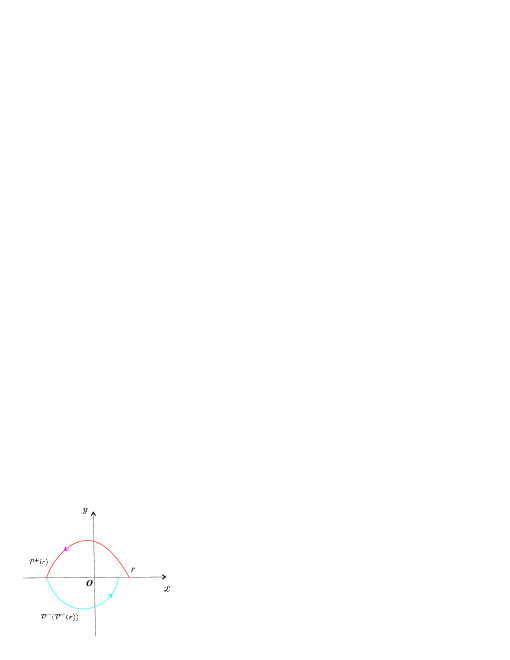
Figure 1. Existence of closed orbits for system $(I)$.

Piecewise smooth system $(I)$ has a polynomial first integral $H_{1}^{+}(x,y)=\frac{a_{1}}{3}y^{3}-\frac{b_{1}}{2}x^{2}$ if $y\geq 0$, and a first integral $H_{1}^{-}(x,y)=\frac{\tilde{a}_{1}}{3}y^{3}-\frac{1}{2}x^{2}$ if $y<0$. Then we have $H_{1}^{+}(r,0)=H_{1}^{+}(\mathcal{P}^{+}(r),0),$ yielding that $\mathcal{P}^{+}(r)=r$. Furthermore, by

$$H_{1}^{-}(\mathcal{P}^{+}(r),0)=H_{1}^{-}(\mathcal{P}_{I}(r),0)$$

we get $\mathcal{P}_{I}(r)=r$, implying that the solution curve of piecewise smooth system $(I)$ through $(r,0)$ is a closed orbit for arbitrary $r>0$. Notice that the origin $O_{1}$ is the unique singularity of piecewise smooth system $(I)$ when $a_{1}<0,b_{1}>0$ and $\tilde{a}_{1}>0$. Therefore, the origin $O_{1}$ of piecewise smooth system $(I)$ is a center if and only if $a_{1}<0,b_{1}>0$ and $\tilde{a}_{1}>0$ and furthermore it is a global center.

Next, in the case $a_{1}<0,b_{1}>0$ and $\tilde{a}_{1}>0$ we prove that the center $O_{1}$ at the origin of piecewise smooth system $(I)$ is not isochronous. Assuming that $\Gamma_{r_{0}}$ is the closed trajectory through $(r_{0},0)$ inside the periodic annulus of the center $O_{1}$, we can define the positive half-period function as $T^{+}(r_{0}):=\int_{\Gamma^{+}_{r_{0}}}~{}dt$ and the negative half-period function as $T^{-}(r_{0}):=\int_{\Gamma^{-}_{r_{0}}}~{}dt,$ where $r_{0}>0$,

$$\Gamma^{+}_{r_{0}}=\{(\rho,\theta)\in\mathbb{R}^{2}~{}|~{}\rho=p^{+}(r_{0},\theta)\}=\{(x,y)\in\mathbb{R}^{2}~{}|~{}y=\Big{(}\frac{3b_{1}}{2a_{1}}(x^{2}-r_{0}^{2})\Big{)}^{\frac{1}{3}}~{}\}$$

and

$$\Gamma^{-}_{r_{0}}=\{(\rho,\theta)\in\mathbb{R}^{2}~{}|~{}\rho=p^{-}(r_{0},\theta)\}=\{(x,y)\in\mathbb{R}^{2}~{}|~{}y=\Big{(}\frac{3}{2\tilde{a}_{1}}(x^{2}-r_{0}^{2})\Big{)}^{\frac{1}{3}}~{}\}.$$

Thus the complete period function associated to piecewise smooth system $(I)$ is given by the sum of these two functions

$$T_{I}(r_{0}) =\oint_{\Gamma_{r_{0}}}~{}dt=T^{+}(r_{0})+T^{-}(r_{0})=\int_{\Gamma^{+}_{r_{0}}}~{}\frac{dx}{a_{1}y^{2}}+\int_{\Gamma^{-}_{r_{0}}}~{}\frac{dx}{\tilde{a}_{1}y^{2}}$$

$$=\int_{r_{0}}^{-r_{0}}~{}\frac{dx}{a_{1}\Big{(}\frac{3b_{1}}{2a_{1}}(x^{2}-r_{0}^{2})\Big{)}^{\frac{2}{3}}}+\int_{-r_{0}}^{r_{0}}~{}\frac{dx}{\tilde{a}_{1}\Big{(}\frac{3}{2\tilde{a}_{1}}(x^{2}-r_{0}^{2})\Big{)}^{\frac{2}{3}}}$$

$$=\beta_{0}r_{0}^{-\frac{1}{3}},$$

where $\beta_{0}=\frac{(\frac{2}{3})^{\frac{5}{3}}\pi^{\frac{3}{2}}\sqrt{3}}{\Gamma(\frac{2}{3})\Gamma(\frac{5}{6})}(-a_{1}^{-\frac{1}{3}}b_{1}^{-\frac{2}{3}}+\tilde{a}_{1}^{-\frac{1}{3}})>0$ and the Gamma function $\Gamma(z)=\int_{0}^{\infty}~{}e^{-s}s^{z-1}~{}ds$. Clearly the period $T_{I}(r_{0})$ of the periodic orbits inside the period annulus of the center $O_{1}$ is monotonic in $r_{0}$ and then it cannot be isochronous. We complete the proof of the theorem. ∎

3. Global structures of piecewise smooth quadratic quasi–homogeneous systems

We will apply the ideal of Poincaré compactification to study the global structures of piecewise smooth quadratic quasi–homogeneous but non–homogeneous systems. Although this theory is usually used in smooth systems, our strategy is to analyze the properties at infinity on half plane one by one, and via the discussion of sliding sets and crossing sets we can summarize the global topological structures of piecewise smooth quadratic quasi–homogeneous systems.

First we briefly remind the procedure of Poincaré compactification [3, 11]. Consider a planar vector field

$$\mathcal{X}=\tilde{P}(x,y)\dfrac{\partial}{\partial x}+\tilde{Q}(x,y)\dfrac{\partial}{\partial y},$$

where $\tilde{P}(x,y)$ and $\tilde{Q}(x,y)$ are polynomials of degree $n$. Set $\mathbb{S}^{2}=\{y=(y_{1},y_{2},y_{3})\in\mathbb{R}^{3}:y_{1}^{2}+y_{2}^{2}+y_{3}^{2}=1\}$, $\mathbb{S}^{1}$ be the equator of $\mathbb{S}^{2}$ and $p(\mathcal{X})$ be the Poincaré compactification of $\mathcal{X}$ on $\mathbb{S}^{2}$. Note that $\mathbb{S}^{1}$ is invariant under the flow of $p(\mathcal{X})$.

We consider the six local charts $U_{i}=\{y\in\mathbb{S}^{2}:y_{i}>0\}$ and $V_{i}=\{y\in\mathbb{S}^{2}:y_{i}<0\}$ where $i=1,2,3$ for the calculation of the expression of $p(\mathcal{X})$. The diffeomorphisms $F_{i}:U_{i}\rightarrow\mathbb{R}^{2}$ and $G_{i}:V_{i}\rightarrow\mathbb{R}^{2}$ for $i=1,2,3$ are the inverses of the central projections from the planes tangent at the points $(1,0,0),(-1,0,0),(0,1,0),(0,-1,0),(0,0,1)$ and $(0,0,-1)$ respectively. We denote by $(u,z)$ the value of $F_{i}(y)$ or $G_{i}(y)$ for any $i=1,2,3$. The expression for $p(\mathcal{X})$ in the local chart $(U_{1},F_{1})$ is given by

$$\dot{u}=z^{n}\left[-u\tilde{P}\left(\dfrac{1}{z},\dfrac{u}{z}\right)+\tilde{Q}\left(\dfrac{1}{z},\dfrac{u}{z}\right)\right],\hskip 8.5359pt\dot{z}=-z^{n+1}\tilde{P}\left(\dfrac{1}{z},\dfrac{u}{z}\right),$$

for $(U_{2},F_{2})$ is

$$\dot{u}=z^{n}\left[\tilde{P}\left(\dfrac{u}{z},\dfrac{1}{z}\right)-u\tilde{Q}\left(\dfrac{u}{z},\dfrac{1}{z}\right)\right],\hskip 8.5359pt\dot{z}=-z^{n+1}\tilde{Q}\left(\dfrac{u}{z},\dfrac{1}{z}\right),$$

and for $(U_{3},F_{3})$ is

$$\dot{u}=\tilde{P}(u,z),\hskip 8.5359pt\dot{z}=\tilde{Q}(u,z).$$

When we study the equilibria at infinitt on the charts $U_{2}\cup V_{2}$, we only need to verify if the origins of these charts are singular points.

Theorem 3.

Piecewise smooth quadratic quasi–homogeneous systems $(I)$, $(II)$ and $(III)$ have totally $8$, $64$ and $36$ global phase portraits respectively.

Proof.

For piecewise smooth system $(I)$, the origin of the corresponding smooth system $(i)$ is a cusp by the proof of Theorem 2. Moreover, in the half plane $y>0$ (resp. $y<0$) the piecewise smooth system $(I)$ has an invariant curve $\frac{a_{1}}{3}y^{3}-\frac{b_{1}}{2}x^{2}=0$ (resp. $\frac{\tilde{a}_{1}}{3}y^{3}-\frac{1}{2}x^{2}=0$) passing through the origin $O_{1}:(0,0)$ when $a_{1}b_{1}>0$ (resp. $\tilde{a}_{1}<0$).

Taking respectively the Poincaré transformations $x=1/z,\,y=u/z$ in the local chart $U_{1}$ and $x=u/z,\,y=1/z$ in the local chart $U_{2}$, smooth system $(i)$ around the equator of the Poincaré sphere can be written respectively in

(3.1) $$\dot{u}=b_{1}z-a_{1}u^{3},\qquad\dot{z}=-a_{1}u^{2}z$$

and

$$\dot{u}=a_{1}-b_{1}u^{2}z,\qquad\dot{z}=-b_{1}uz^{2}.$$

Then singularities at infinity of system $(i)$ only exist on the $x$-axis, whose corresponding equilibrium in the local chart $U_{1}$ (the origin of (3.1)) is a node by [11, Theorem 3.5]. Besides, system $(i)$ has the polynomial first integral $H_{1}^{+}(x,y)=\frac{a_{1}}{3}y^{3}-\frac{b_{1}}{2}x^{2}$. Therefore, it is not difficult to get global phase portraits of smooth system $(i)$.

Notice that piecewise smooth system $(I)$ is invariant under the change $(x,y)\to(-x,y)$ after a time rescaling $d\tau\to-d\tau$, so we only need to consider phase portraits in the half plane $x\geq 0$. From (2.6) and (2.9), we know that the crossing set $\mathcal{L}_{c}^{I}=\{(x,y)\in\mathbb{R}^{2}|~{}y=0,x\neq 0\}$ if $b_{1}>0$ and the sliding set $\mathcal{L}_{s}^{I}=\{(x,y)\in\mathbb{R}^{2}|~{}y=0\}$ if $b_{1}<0$. The origin $O_{1}$ is the unique singular sliding point of piecewise smooth system $(I)$. Hence when $b_{1}>0$, the global phase portraits of piecewise smooth system $(I)$ can be obtained by the global phase portraits of system $(i)$ in the half plane $y>0$ and $y<0$ respectively, where four cases $b_{1}>0,a_{1}>0,\tilde{a}_{1}>0$; $b_{1}>0,a_{1}>0,\tilde{a}_{1}<0$; $b_{1}>0,a_{1}<0,\tilde{a}_{1}<0$ and $b_{1}>0,a_{1}<0,\tilde{a}_{1}>0$ are considered. Notice that the whole plane is the period annulus of the center at the origin of system $(I)$ if $b_{1}>0,a_{1}<0,\tilde{a}_{1}>0$. There exist infinitely many homoclinic loops connecting with the singularities at infinity on the $x$-axis and an eight-shape heteroclinic loop connecting with the singularities at infinity on the $x$-axis and the origin if $b_{1}>0,a_{1}>0,\tilde{a}_{1}<0$. In contrast, when $b_{1}<0$ the whole $x$-axis is the sliding set and each point except the origin on the $x$-axis is a ”colliding” point of orbits, i.e., the orbit connecting the point from the half plane $y>0$ is along the opposite direction with that from the half plane $y<0$. Thus, neither closed orbits nor homoclinic loops could exist if $b_{1}<0$. For $b_{1}<0$, we research the global phase portraits of piecewise smooth system $(I)$ in four cases: $a_{1}>0,\tilde{a}_{1}>0$; $a_{1}>0,\tilde{a}_{1}<0$; $a_{1}<0,\tilde{a}_{1}<0$ and $a_{1}<0,\tilde{a}_{1}>0$. Note that in the case $b_{1}<0,a_{1}>0,\tilde{a}_{1}>0$ it seems that the origin is surrounded by closed orbits but it is not true, since the direction of upper half of each oval is clockwise but the direction of the lower half is anticlockwise. Thus the ovals existing in the case $b_{1}<0,a_{1}<0,\tilde{a}_{1}>0$ are not homoclinic loops actually by the similar reason. Thus we obtain $8$ global phase portraits for piecewise smooth system $(I)$ under above $8$ parameter conditions.

We next investigate the piecewise smooth system $(II)$ for its global structures. Using Theorem 3.5 of [11], the origin of smooth system $(ii)$ is a saddle if $a_{2}b_{22}<0$, and its neighborhood consists of a hyperbolic sector and an elliptic sector if $a_{2}b_{22}>0$. Taking respectively the Poincaré transformations $x=1/z,\,y=u/z$ in the local chart $U_{1}$ and $x=u/z,\,y=1/z$ in the local chart $U_{2}$, system $(ii)$ around the equator of the Poincaré sphere can be written respectively as

(3.2) $$\dot{u}=b_{21}z+(b_{22}-a_{2})u^{2},\qquad\dot{z}=-a_{2}uz$$

and

(3.3) $$\dot{u}=(a_{2}-b_{22})u-b_{21}u^{2}z,\qquad\dot{z}=-b_{22}z-b_{21}uz^{2}.$$

Therefore, there exist singularities of system $(ii)$ located at the infinity of both the $x$-axis and the $y$-axis if $b_{22}\neq a_{2}$, which are associated to the origins of system (3.2) and system (3.3) respectively. It is easy to see that the origin of system (3.3) is a saddle if $(b_{22}-a_{2})b_{22}<0$ and a node if $(b_{22}-a_{2})b_{22}>0$. Applying [11, Theorem 3.5], the origin of system (3.2) is a saddle if $(b_{22}-a_{2})a_{2}>0$ and its neighborhood consists of a hyperbolic sector and an elliptic sector if $(b_{22}-a_{2})a_{2}<0$. When $b_{22}=a_{2}$, the infinity is full up with singularities and there exists a unique orbit connecting with each point at infinity.

From (2.12) and (2.15), we get that the crossing set $\mathcal{L}_{c}^{II}=\{(x,y)\in\mathbb{R}^{2}|~{}y=0,x\neq 0\}$ if $b_{21}>0$ and the sliding set $\mathcal{L}_{s}^{II}=\{(x,y)\in\mathbb{R}^{2}|~{}y=0\}$ if $b_{21}<0$ for piecewise smooth system $(II)$. The origin $O_{2}:(0,0)$ is the unique singular sliding point of piecewise smooth system $(II)$. Moreover, system $(II)$ has a first integral

$$H_{2}^{+}(x,y)=\frac{-2b_{21}x+(a_{2}-2b_{22})y^{2}}{x^{\frac{2b_{22}}{a_{2}}}(-2b_{22}+a_{2})}\qquad(resp.=\frac{-b_{21}x\ln x+b_{22}y^{2}}{b_{22}x})$$

when $y\geq 0$ and $a_{2}\neq 2b_{22}$ (resp. $a_{2}=2b_{22}$), and a first integral

$$H_{2}^{-}(x,y)=\frac{-2x+(\tilde{a}_{2}-2)y^{2}}{x^{\frac{2}{\tilde{a}_{2}}}(-2+\tilde{a}_{2})}\qquad(resp.=\frac{x\ln x-y^{2}}{x})$$

when $y<0$ and $\tilde{a}_{2}\neq 2$ (resp. $\tilde{a}_{2}=2$). Similar to the research of system $(I)$, the global phase portraits of piecewise smooth system $(II)$ can be obtained by the global phase portraits of system $(ii)$ in the half planes $y>0$ and $y<0$ together with the dynamics on the crossing set and sliding set, where $64$ subcases correspond to parameter conditions obtained by the signs of $b_{21}$, $b_{22}-a_{2}$, $b_{22}$, $a_{2}$, $\tilde{a}_{2}$ and $\tilde{a}_{2}-1$.

In order to research the global dynamics of piecewise smooth system $(III)$, we need find global dynamics of smooth system $(iii)$. Obviously, the origin $O_{3}:(0,0)$ of system $(iii)$ is a saddle if $a_{31}b_{3}<0$ and a node if $a_{31}b_{3}>0$.

In the local charts $U_{1}$ and $U_{2}$ of the Poincaré sphere, system $(iii)$ becomes

(3.4) $$\dot{u}=(b_{3}-a_{31})uz-a_{32}u^{3},\qquad\dot{z}=-a_{31}z^{2}-a_{32}u^{2}z$$

and

$$\dot{u}=a_{32}+(a_{31}-b_{3})uz,\qquad\dot{z}=-b_{3}z^{2},$$

respectively. Then there exist singularities at infinity of system $(iii)$ only located on the $x$-axis, which are associated to the origin of (3.4), a high degenerate equilibrium. More precisely, the neighborhood of the origin of (3.4) consists of two elliptic sectors and one parabolic sector if $a_{31}b_{3}<0$, two hyperbolic sectors and two parabolic sectors if $0<a_{31}b_{3}\leq 2b_{3}^{2}$, and two hyperbolic sectors and four parabolic sectors if $a_{31}b_{3}>2b_{3}^{2}$ by applying results of Reyn [31, Figures 8.3c-8.3d].

The sliding set of piecewise smooth system $(III)$ is the whole $x$-axis from (2.16), which is filled with singular sliding points. Except the origin and singularities of system $(III)$ located at the infinity of the $x$-axis, no orbits connect with the point in the $x$-axis from the half planes $y>0$ or $y<0$. Hence, neither closed orbits nor sliding closed orbits could exist. There exist no homoclinic loops in a bounded region, that is, a homoclinic loop has to pass by a singularity at infinity of the $x$-axis if it exists. Besides, system $(III)$ has a first integral

$$H_{3}^{+}(x,y)=\frac{(a_{31}-2b_{3})x+a_{32}y^{2}}{y^{\frac{a_{31}}{b_{3}}}(-2b_{3}+a_{31})}\qquad(resp.=-\frac{a_{32}y^{2}\ln y-b_{3}x}{b_{3}y^{2}})$$

when $y\geq 0$ and $a_{31}\neq 2b_{3}$ (resp. $a_{31}=2b_{3}$), and a first integral

$$H_{3}^{-}(x,y)=\frac{(\tilde{a}_{31}-2)x+y^{2}}{y^{\tilde{a}_{31}}(-2+\tilde{a}_{31})},\qquad(resp.=-\frac{y^{2}\ln y-x}{y^{2}})$$

when $y<0$ and $\tilde{a}_{31}\neq 2$ (resp. $\tilde{a}_{31}=2$). From an analogous discussion of system $(I)$ in the case $b_{1}<0$, the above analysis of system $(III)$ provides enough preparation for studying the global structure of piecewise smooth system $(III)$ and we have its 36 global phase portraits by the signs of $a_{31}$, $b_{3}$, $a_{31}-2b_{3}$, $a_{32}$, $\tilde{a}_{31}$ and $\tilde{a}_{31}-2$ respectively.

Summarizing the above investigation, we can obtain global dynamics of piecewise smooth quadratic quasi–homogeneous systems $(I)$-$(III)$. The proof is completed. ∎

Here for simplicity, we only present details of topological phase portraits of piecewise smooth system $(III)$ and omit that of systems $(I)$ and $(II)$. The parameter conditions associated to cases $(1)$-$(36)$ are give in Table 1. Remark that we will not consider invertible changes which transform the half plane $y>0$ into the half plane $y<0$ for the topological equivalence of global phase portraits, in the sense that the vector fields of piecewise smooth systems are different in the half planes $y>0$ and $y<0$.

Note that for smooth quadratic quasi–homogeneous system $(i)$ (resp. $(ii)$, $(iii)$) there only exists $1$ (resp. $4$, $3$) global phase portrait without taking into account the direction of the time, but piecewise smooth quadratic quasi–homogeneous system $(I)$ (resp. $(II)$, $(III)$) has $8$ (resp. $64$, $36$) global phase portraits. Thus piecewise smooth quadratic quasi–homogeneous systems can exhibit more complicated and richer dynamics than the smooth ones.

cases	Parameter conditions
(1)	$a_{31}<0$, $b_{3}<0$, $a_{31}\geq 2b_{3}$, $a_{32}<0$ and $\tilde{a}_{31}>2$
(2)	$a_{31}<0$, $b_{3}<0$, $a_{31}\geq 2b_{3}$, $a_{32}<0$ and $0<\tilde{a}_{31}\leq 2$
(3)	$a_{31}<0$, $b_{3}<0$, $a_{31}\geq 2b_{3}$, $a_{32}<0$ and $\tilde{a}_{31}<0$
(4)	$a_{31}<0$, $b_{3}<0$, $a_{31}\geq 2b_{3}$, $a_{32}>0$ and $\tilde{a}_{31}>2$
(5)	$a_{31}<0$, $b_{3}<0$, $a_{31}\geq 2b_{3}$, $a_{32}>0$ and $0<\tilde{a}_{31}\leq 2$
(6)	$a_{31}<0$, $b_{3}<0$, $a_{31}\geq 2b_{3}$, $a_{32}>0$ and $\tilde{a}_{31}<0$
(7)	$a_{31}<0$, $b_{3}<0$, $a_{31}<2b_{3}$, $a_{32}>0$ and $\tilde{a}_{31}>2$
(8)	$a_{31}<0$, $b_{3}<0$, $a_{31}<2b_{3}$, $a_{32}>0$ and $0<\tilde{a}_{31}\leq 2$
(9)	$a_{31}<0$, $b_{3}<0$, $a_{31}<2b_{3}$, $a_{32}>0$ and $\tilde{a}_{31}<0$
(10)	$a_{31}<0$, $b_{3}<0$, $a_{31}<2b_{3}$, $a_{32}<0$ and $\tilde{a}_{31}>2$
(11)	$a_{31}<0$, $b_{3}<0$, $a_{31}<2b_{3}$, $a_{32}<0$ and $0<\tilde{a}_{31}\leq 2$
(12)	$a_{31}<0$, $b_{3}<0$, $a_{31}<2b_{3}$, $a_{32}<0$ and $\tilde{a}_{31}<0$
(13)	$a_{31}>0$, $b_{3}>0$, $a_{31}\leq 2b_{3}$, $a_{32}<0$ and $\tilde{a}_{31}>2$
(14)	$a_{31}>0$, $b_{3}>0$, $a_{31}\leq 2b_{3}$, $a_{32}<0$ and $0<\tilde{a}_{31}\leq 2$
(15)	$a_{31}>0$, $b_{3}>0$, $a_{31}\leq 2b_{3}$, $a_{32}<0$ and $\tilde{a}_{31}<0$
(16)	$a_{31}>0$, $b_{3}>0$, $a_{31}\leq 2b_{3}$, $a_{32}>0$ and $\tilde{a}_{31}>2$
(17)	$a_{31}>0$, $b_{3}>0$, $a_{31}\leq 2b_{3}$, $a_{32}>0$ and $0<\tilde{a}_{31}\leq 2$
(18)	$a_{31}>0$, $b_{3}>0$, $a_{31}\leq 2b_{3}$, $a_{32}>0$ and $\tilde{a}_{31}<0$
(19)	$a_{31}>0$, $b_{3}>0$, $a_{31}>2b_{3}$, $a_{32}<0$ and $\tilde{a}_{31}>2$
(20)	$a_{31}>0$, $b_{3}>0$, $a_{31}>2b_{3}$, $a_{32}<0$ and $0<\tilde{a}_{31}\leq 2$
(21)	$a_{31}>0$, $b_{3}>0$, $a_{31}>2b_{3}$, $a_{32}<0$ and $\tilde{a}_{31}<0$
(22)	$a_{31}>0$, $b_{3}>0$, $a_{31}>2b_{3}$, $a_{32}>0$ and $\tilde{a}_{31}>2$
(23)	$a_{31}>0$, $b_{3}>0$, $a_{31}>2b_{3}$, $a_{32}>0$ and $0<\tilde{a}_{31}\leq 2$
(24)	$a_{31}>0$, $b_{3}>0$, $a_{31}>2b_{3}$, $a_{32}>0$ and $\tilde{a}_{31}<0$
(25)	$a_{31}>0$, $b_{3}<0$, $a_{32}<0$ and $\tilde{a}_{31}>2$
(26)	$a_{31}>0$, $b_{3}<0$, $a_{32}<0$ and $0<\tilde{a}_{31}\leq 2$
(27)	$a_{31}>0$, $b_{3}<0$, $a_{32}<0$ and $\tilde{a}_{31}<0$
(28)	$a_{31}>0$, $b_{3}<0$, $a_{32}>0$ and $\tilde{a}_{31}>2$
(29)	$a_{31}>0$, $b_{3}<0$, $a_{32}>0$ and $0<\tilde{a}_{31}\leq 2$
(30)	$a_{31}>0$, $b_{3}<0$, $a_{32}>0$ and $\tilde{a}_{31}<0$
(31)	$a_{31}<0$, $b_{3}>0$, $a_{32}<0$ and $\tilde{a}_{31}>2$
(32)	$a_{31}<0$, $b_{3}>0$, $a_{32}<0$ and $0<\tilde{a}_{31}\leq 2$
(33)	$a_{31}<0$, $b_{3}>0$, $a_{32}<0$ and $\tilde{a}_{31}<0$
(34)	$a_{31}<0$, $b_{3}>0$, $a_{32}>0$ and $\tilde{a}_{31}>2$
(35)	$a_{31}<0$, $b_{3}>0$, $a_{32}>0$ and $0<\tilde{a}_{31}\leq 2$
(36)	$a_{31}<0$, $b_{3}>0$, $a_{32}>0$ and $\tilde{a}_{31}<0$

Table 1. Parameter conditions for global phase portraits of system $(III)$.

From the global dynamics of piecewise smooth systems $(I)$-$(III)$, we can research the global bifurcation and unfolding of all special orbits including homoclinic loops (or heteroclinic loops), closed orbits, equilibria and equilibria at infinity for the systems. For example, the unfoldings are presented in phase portraits (2) and (3) if we choose $\mu_{1}=\tilde{a}_{31}$ as an unfolding parameter. A homoclinic (or heteroclinic) bifurcation happens when $\mu_{1}$ passes through zero. More precisely, when $\mu_{1}>0$ there exist infinitely many heteroclinic loops connecting with the origin and equilibria at infinity on the $x$-axis, and when $\mu_{1}<0$ some heteroclinic orbits in the half plane $y<0$ become homoclinic loops connecting with the equilibria at infinity on the $x$-axis. If we choose $\mu_{2}=a_{32}$ as another unfolding parameter, we find that the heteroclinic loops burst out when $\mu_{2}$ varies from negative to positive by phase portraits (2) and (5). At the same time it can be observed clearly the change of sectors in a neighborhood of equilibria and equilibria at infinity, which exhibits bifurcations of equilibria. We can also notice other global and local bifurcations if we choose $b_{3}$, $a_{31}-2b_{3}$, $a_{31}$ and $\tilde{a}_{31}-2$ as unfolding parameters for piecewise smooth system $(III)$.

4. Limit cycle bifurcations by perturbing piecewise smooth quadratic quasi–homogeneous systems

From Theorem 2, only system $(I)$ of all piecewise smooth quadratic quasi-homogeneous systems has a center at the origin, which is global if it exists. In this section we research the bifurcation of limit cycles by perturbing piecewise smooth quadratic quasi–homogeneous system $(I)$ with arbitrary piecewise polynomials of degree $n\in\mathbb{N}$, where $\mathbb{N}=\mathbb{Z}_{+}\cup\{0\}$.

Consider the following one-parametric family of piecewise smooth systems

(4.1) $$\dot{x}=H_{y}(x,y)+\epsilon f(x,y),\qquad\dot{y}=-H_{x}(x,y)+\epsilon g(x,y),$$

where $\epsilon\in\mathbb{R}$ is the small perturbation parameter,

$$H(x,y)=\begin{cases}H^{+}(x,y):=H_{1}^{+}(x,y)=\frac{a_{1}}{3}y^{3}-\frac{b_{1}}{2}x^{2},~{}\mbox{ if }~{}y\geq 0,\\ H^{-}(x,y):=H_{1}^{-}(x,y)=\frac{\tilde{a}_{1}}{3}y^{3}-\frac{1}{2}x^{2},~{}\mbox{ if }~{}y<0,\end{cases}$$

$$f(x,y)=\begin{cases}f^{+}(x,y)=\sum_{i+j=0}^{n}c_{ij}^{+}~{}x^{i}y^{j},~{}\mbox{ if }~{}y\geq 0,\\ f^{-}(x,y)=\sum_{i+j=0}^{n}c_{ij}^{-}~{}x^{i}y^{j},~{}\mbox{ if }~{}y<0,\end{cases}$$

$$g(x,y)=\begin{cases}g^{+}(x,y)=\sum_{i+j=0}^{n}d_{ij}^{+}~{}x^{i}y^{j},~{}\mbox{ if }~{}y\geq 0,\\ g^{-}(x,y)=\sum_{i+j=0}^{n}d_{ij}^{-}~{}x^{i}y^{j},~{}\mbox{ if }~{}y<0\end{cases}$$

for arbitrary $c_{ij}^{\pm},d_{ij}^{\pm}\in\mathbb{R}$, and $a_{1}<0,b_{1}>0$ and $\tilde{a}_{1}>0$. Our aim is to give the maximum number of limit cycles in terms of $n$ which can bifurcate from the periodic orbits of the center at the origin of system $(I)$ with $\epsilon=0$, inside the family (4.1) for nonzero $\epsilon$.

We will use Melnikov method to investigate the number of bifurcated limit cycles from system (4.1). Let

$$L_{h}^{+}=\{(x,y)\in\mathbb{R}^{2}\mid H_{1}^{+}(x,y)=-\frac{h}{2},~{}h>0\},~{}\mbox{ if }~{}y\geq 0,$$

$$L_{h}^{-}=\{(x,y)\in\mathbb{R}^{2}\mid H_{1}^{-}(x,y)=-\frac{h}{2b_{1}},~{}h>0\},~{}\mbox{ if }~{}y<0.$$

Then the family of periodic orbits of system (4.1) with $\epsilon=0$ is presented by $L_{h}=L_{h}^{+}\cup L_{h}^{-}$, where $h>0$.

Using the idea in [27] for piecewise smooth system with a discontinuous line the $y$-axis, we have the first order Melnikov function for system (4.1) along the family of periodic orbits $L_{h}$, which is

(4.2) $$\qquad\qquad M(h,\epsilon)=\frac{H_{x}^{+}(A)}{H_{x}^{-}(A)}\Big{(}\frac{H_{x}^{-}(B)}{H_{x}^{+}(B)}\int_{L_{h}^{+}}(g^{+}dx-f^{+}dy)+\int_{L_{h}^{-}}(g^{-}dx-f^{-}dy)\Big{)},$$

where points $A=(\sqrt{\frac{h}{b_{1}}},0)$ and $B=(-\sqrt{\frac{h}{b_{1}}},0)$, as shown in Figure 2.

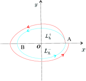
Figure 2. The closed orbit of system $(I)$ and its perturbation.

Lemma 4.

For piecewise smooth system (4.1), we have the first order Melnikov function

(4.3) $$M(h,\epsilon)=\sum_{2k+j=0}^{n}\xi_{2k,j}~{}h^{k+\frac{j}{3}+\frac{1}{2}},$$

where coefficients $\xi_{2k,j}$ are given in (4.29).

Proof.

Firstly, we compute that $H_{x}^{+}(A)=-b_{1}\sqrt{\frac{h}{b_{1}}}$, $H_{x}^{-}(A)=-\sqrt{\frac{h}{b_{1}}}$, $H_{x}^{-}(B)=\sqrt{\frac{h}{b_{1}}}$ and $H_{x}^{+}(B)=b_{1}\sqrt{\frac{h}{b_{1}}}$ in (4.2).

Restricted on $L_{h}^{+}$ and $L_{h}^{-}$, we solve $y=\sqrt[3]{\frac{3}{2a_{1}}(-h+b_{1}x^{2})}$ and $y=\sqrt[3]{\frac{3}{2\tilde{a}_{1}}(-\frac{h}{b_{1}}+x^{2})}$, respectively. Then for $i,j\in\mathbb{N}$ we calculate

(4.7) $$\begin{array}[]{lll}\int_{L_{h}^{+}}~{}x^{i}y^{j}dx&=(\frac{3}{2a_{1}})^{\frac{j}{3}}\int_{\sqrt{\frac{h}{b_{1}}}}^{-\sqrt{\frac{h}{b_{1}}}}x^{i}(-h+b_{1}x^{2})^{\frac{j}{3}}dx\\ &=-2(\frac{3}{2a_{1}})^{\frac{j}{3}}\int_{0}^{\sqrt{\frac{h}{b_{1}}}}x^{2k}(-h+b_{1}x^{2})^{\frac{j}{3}}dx\\ &=\hat{d}_{2k,j}^{+}~{}h^{k+\frac{j}{3}+\frac{1}{2}},\end{array}$$

(4.12) $$\begin{array}[]{lll}\int_{L_{h}^{+}}~{}x^{i}y^{j}dy&=\frac{b_{1}}{a_{1}}\int_{L_{h}^{+}}~{}x^{i+1}y^{j-2}dx\\ &=\frac{b_{1}}{a_{1}}(\frac{3}{2a_{1}})^{\frac{j-2}{3}}\int_{\sqrt{\frac{h}{b_{1}}}}^{-\sqrt{\frac{h}{b_{1}}}}x^{i+1}(-h+b_{1}x^{2})^{\frac{j-2}{3}}dx\\ &=-2\frac{b_{1}}{a_{1}}(\frac{3}{2a_{1}})^{\frac{j-2}{3}}\int_{0}^{\sqrt{\frac{h}{b_{1}}}}x^{2k+2}(-h+b_{1}x^{2})^{\frac{j-2}{3}}dx\\ &=\hat{c}_{2k+1,j}^{+}~{}h^{k+\frac{j+1}{3}+\frac{1}{2}},\end{array}$$

(4.16) $$\begin{array}[]{lll}\int_{L_{h}^{-}}~{}x^{i}y^{j}dx&=(\frac{3}{2\tilde{a}_{1}})^{\frac{j}{3}}\int_{-\sqrt{\frac{h}{b_{1}}}}^{\sqrt{\frac{h}{b_{1}}}}x^{i}(x^{2}-\frac{h}{b_{1}})^{\frac{j}{3}}dx\\ &=2(\frac{3}{2\tilde{a}_{1}})^{\frac{j}{3}}\int_{0}^{\sqrt{\frac{h}{b_{1}}}}x^{2k}(x^{2}-\frac{h}{b_{1}})^{\frac{j}{3}}dx\\ &=\hat{d}_{2k,j}^{-}~{}h^{k+\frac{j}{3}+\frac{1}{2}}\end{array}$$

and

(4.21) $$\begin{array}[]{lll}\int_{L_{h}^{-}}~{}x^{i}y^{j}dy&=\frac{1}{\tilde{a}_{1}}\int_{L_{h}^{-}}~{}x^{i+1}y^{j-2}dx\\ &=\frac{1}{\tilde{a}_{1}}(\frac{3}{2\tilde{a}_{1}})^{\frac{j-2}{3}}\int_{-\sqrt{\frac{h}{b_{1}}}}^{\sqrt{\frac{h}{b_{1}}}}x^{i+1}(x^{2}-\frac{h}{b_{1}})^{\frac{j-2}{3}}dx\\ &=2\frac{1}{\tilde{a}_{1}}(\frac{3}{2\tilde{a}_{1}})^{\frac{j-2}{3}}\int_{0}^{\sqrt{\frac{h}{b_{1}}}}x^{2k+2}(x^{2}-\frac{h}{b_{1}})^{\frac{j-2}{3}}dx\\ &=\hat{c}_{2k+1,j}^{-}~{}h^{k+\frac{j+1}{3}+\frac{1}{2}}\end{array}$$

where $k\in\mathbb{N}$,

(4.26) $$\begin{array}[]{lll}\hat{d}_{2k,j}^{+}&=-2(\frac{3}{2a_{1}})^{\frac{j}{3}}(\frac{1}{b_{1}})^{k+\frac{1}{2}}\int_{0}^{1}x^{2k}(-1+x^{2})^{\frac{j}{3}}dx,\\ \hat{c}_{2k+1,j}^{+}&=-2\frac{b_{1}}{a_{1}}(\frac{3}{2a_{1}})^{\frac{j-2}{3}}(\frac{1}{b_{1}})^{k+1+\frac{1}{2}}\int_{0}^{1}x^{2k+2}(-1+x^{2})^{\frac{j-2}{3}}dx,\\ \hat{d}_{2k,j}^{-}&=2(\frac{3}{2\tilde{a}_{1}})^{\frac{j}{3}}(\frac{1}{b_{1}})^{k+\frac{j}{3}+\frac{1}{2}}\int_{0}^{1}x^{2k}(-1+x^{2})^{\frac{j}{3}}dx,\\ \hat{c}_{2k+1,j}^{-}&=2\frac{1}{\tilde{a}_{1}}(\frac{3}{2\tilde{a}_{1}})^{\frac{j-2}{3}}(\frac{1}{b_{1}})^{k+\frac{j+1}{3}+\frac{1}{2}}\int_{0}^{1}x^{2k+2}(-1+x^{2})^{\frac{j-2}{3}}dx.\end{array}$$

Notice that $\hat{d}_{2k,j}^{+}\hat{c}_{2k+1,j}^{+}\hat{d}_{2k,j}^{-}\hat{c}_{2k+1,j}^{-}\neq 0$, $\int_{L_{h}^{\pm}}~{}x^{i}y^{j}dx=0$ for odd $i$ and $\int_{L_{h}^{\pm}}~{}x^{i}y^{j}dy=0$ for even $i$.

Substituting (4.7)–(4.21) into the formula (4.2), we obtain the Melnikov function of system (4.1) as

$$M(h,\epsilon) =b_{1}\Big{(}\frac{1}{b_{1}}\int_{L_{h}^{+}}(g^{+}dx-f^{+}dy)+\int_{L_{h}^{-}}(g^{-}dx-f^{-}dy)\Big{)},$$

$$=\int_{L_{h}^{+}}\Big{(}\sum_{i+j=0}^{n}d_{ij}^{+}~{}x^{i}y^{j}dx-\sum_{i+j=0}^{n}c_{ij}^{+}~{}x^{i}y^{j}dy\Big{)}$$

$$\qquad+b_{1}\int_{L_{h}^{-}}\Big{(}\sum_{i+j=0}^{n}d_{ij}^{-}~{}x^{i}y^{j}dx-\sum_{i+j=0}^{n}c_{ij}^{-}~{}x^{i}y^{j}dy\Big{)}$$

$$=h^{\frac{1}{2}}\Big{(}\sum_{2k+j=0}^{n}d_{2k,j}^{+}~{}\hat{d}_{2k,j}^{+}~{}h^{k+\frac{j}{3}}-\sum_{2k+1+j=0}^{n}c_{2k+1,j}^{+}~{}\hat{c}_{2k+1,j}^{+}~{}h^{k+\frac{j+1}{3}}\Big{)}$$

$$\qquad+b_{1}h^{\frac{1}{2}}\Big{(}\sum_{2k+j=0}^{n}d_{2k,j}^{-}~{}\hat{d}_{2k,j}^{-}~{}h^{k+\frac{j}{3}}-\sum_{2k+1+j=0}^{n}c_{2k+1,j}^{-}~{}\hat{c}_{2k+1,j}^{-}~{}h^{k+\frac{j+1}{3}}\Big{)}$$

$$=h^{\frac{1}{2}}\Big{(}\sum_{2k+j=0}^{n}d_{2k,j}^{+}~{}\hat{d}_{2k,j}^{+}~{}h^{k+\frac{j}{3}}-\sum_{2k+j=0}^{n}c_{2k+1,j-1}^{+}~{}\hat{c}_{2k+1,j-1}^{+}~{}h^{k+\frac{j}{3}}\Big{)}$$

$$\qquad+b_{1}h^{\frac{1}{2}}\Big{(}\sum_{2k+j=0}^{n}d_{2k,j}^{-}~{}\hat{d}_{2k,j}^{-}~{}h^{k+\frac{j}{3}}-\sum_{2k+j=0}^{n}c_{2k+1,j-1}^{-}~{}\hat{c}_{2k+1,j-1}^{-}~{}h^{k+\frac{j}{3}}\Big{)}$$

$$=h^{\frac{1}{2}}\sum_{2k+j=0}^{n}\xi_{2k,j}~{}h^{k+\frac{j}{3}},$$

where $k\in\mathbb{N}$,

(4.29) $$\begin{array}[]{lll}\xi_{2k,j}&=&d_{2k,j}^{+}~{}\hat{d}_{2k,j}^{+}-c_{2k+1,j-1}^{+}~{}\hat{c}_{2k+1,j-1}^{+}\\ &&~{}+b_{1}d_{2k,j}^{-}~{}\hat{d}_{2k,j}^{-}-b_{1}c_{2k+1,j-1}^{-}~{}\hat{c}_{2k+1,j-1}^{-}\end{array}$$

and $\hat{d}_{2k,j}^{+},\hat{c}_{2k+1,j}^{+},\hat{d}_{2k,j}^{-},\hat{c}_{2k+1,j}^{-}$ are displayed in (4.26). Therefore, (4.3) is proved. ∎

In order to determine how many limit cycles the piecewise smooth system (4.1) can have, we analyze zeros of Melnikov function (4.3). For convenience, we set $h=\hat{h}^{6}$ and get from (4.3) that

(4.30) $$M(\hat{h},\epsilon)=\hat{h}^{3}\sum_{2k+j=0}^{n}\xi_{2k,j}~{}\hat{h}^{6k+2j}=\hat{h}^{3}\sum_{i+j=0}^{n}\xi_{i,j}~{}\hat{h}^{3i+2j},$$

where $i$ is even.

The zero problem of $M(h,\epsilon)$ is transferred to determine the cardinal of the set

$$\mathcal{S}(n)=\{3i+2j:~{}0\leq i+j\leq n,~{}i~{}~{}\mbox{even},~{}i,j\in\mathbb{N}\}.$$

That is, we need to find how many different elements exist in the set $\mathcal{S}(n)$.

We denote a trapezoid by

$$\Upsilon_{1}(n)=\{(i,j):~{}0\leq i+j\leq n,~{}j<3,~{}i~{}~{}\mbox{even},~{}i,j\in\mathbb{N}\},$$

and a set by

$$\Upsilon(n)=\{3i+2j:~{}0\leq i+j\leq n,~{}j<3,~{}i~{}~{}\mbox{even},~{}i,j\in\mathbb{N}\}.$$

The cardinal of the set $\mathcal{S}(n)$ is given in the following lemma by applying a similar ideal in [18] for smooth quasi–homogeneous polynomial differential systems.

Lemma 5.

$\mathcal{S}(n)=\Upsilon(n)$.

Proof.

Obviously we have $\mathcal{S}(n)\supset\Upsilon(n)$. We only need to prove that $\mathcal{S}(n)\subset\Upsilon(n)$.

Let $3i+2j$ be an arbitrary element in $\mathcal{S}(n)$ such that $j\geq 3$ and $i$ is even. Then there exists $\iota\in\mathbb{Z}_{+}$ satisfying $3\iota\leq j<3(\iota+1)$. We have

$$3i+2j=3(i+2\iota)+2(j-3\iota)=3i_{1}+2j_{1},$$

where even $i_{1}=i+2\iota\geq 0$, $0\leq j_{1}=j-3\iota<3$ and $0\leq i_{1}+j_{1}=i+j-\iota\leq n$, implying $3i_{1}+2j_{1}\in\Upsilon(n)$ and $3i+2j\in\Upsilon(n)$. Hence $\mathcal{S}(n)\subset\Upsilon(n)$. ∎

Remark that from Lemma 5 all the values of $3i+2j$ for the degrees of $\hat{h}$ in (4.30) are taken exactly by points on the trapezoid $\Upsilon_{1}(n)$.

We need use the following version of the Descartes Theorem proved in [6] to judge real zeros of the Melnikov function.

Theorem 6 (Descartes theorem).

Consider the real polynomial $q(x)=a_{i_{1}}x^{i_{1}}+a_{i_{2}}x^{i_{2}}+\ldots+a_{i_{r}}x^{i_{r}}$ with $0=i_{1}<i_{2}<\ldots<i_{r}$. If $a_{i_{j}}a_{i_{j+1}}<0,$ we say that we have a variation of sign. If the number of variations of signs is $m,$ then the polynomial $q(x)$ has at most $m$ positive real roots. Furthermore, always we can choose the coefficients of the polynomial $q(x)$ in such a way that $q(x)$ has exactly $r-1$ positive real roots.

Let $\Xi(n)$ denote the maximal number of limit cycles, which are produced in piecewise smooth system (4.1) and bifurcated from the period solutions of piecewise smooth quadratic quasi–homogeneous system $(I)$ by taking into account the zeros of the first order Melnikov function.

Theorem 7.

For piecewise smooth quadratic quasi–homogeneous system $(I)$ perturbed inside the class of all piecewise smooth polynomial differential systems of degree $n$ when $a_{1}<0,b_{1}>0$ and $\tilde{a}_{1}>0$, the number $\Xi(n)=2[\frac{n+1}{2}]+[\frac{n-1}{2}]-1$ (resp. $\Xi(n)=2[\frac{n}{2}]+[\frac{n+2}{2}]-1$) if $n$ is odd (resp. even) by the first order Melnikov function. Moreover, there exist perturbations of piecewise smooth polynomial systems of degree $n$ in (4.1) with exactly $\Xi(n)$ limit cycles.

Proof.

From the expression of the first order Melnikov function (4.30) and Theorem 6, we get that $\Xi(n)$ is equal to $|\mathcal{S}(n)|-1$, where $|\mathcal{S}(n)|$ is the cardinal of the set $\mathcal{S}(n)$. Applying Lemma 5 we have $\Xi(n)=|\Upsilon(n)|-1$.

Besides, all the values of the function $3i+2j$ are different for different points on the trapezoid $\Upsilon_{1}(n)$. In fact, if $3i+2j=3\tilde{i}+2\tilde{j}$ for both $(i,j)$ and $(\tilde{i},\tilde{j})$ in $\Upsilon_{1}(n)$, we have $3(i-\tilde{i})=2(\tilde{j}-j)$, yielding that $3|(\tilde{j}-j)$. Because $0\leq\tilde{j},j<3$, we get $\tilde{j}-j=0$ and furthermore $i=\tilde{i}$. Therefore, each of all values of the set $\Upsilon(n)$ is taken exactly once by one point on the trapezoid $\Upsilon_{1}(n)$.

Taking $j=0,1,2$ respectively, we calculate

$$|\Upsilon(n)|=[\frac{n+1}{2}]+[\frac{n+1}{2}]+[\frac{n-1}{2}]=2[\frac{n+1}{2}]+[\frac{n-1}{2}]$$

if $n$ is odd and

$$|\Upsilon(n)|=[\frac{n+2}{2}]+[\frac{n}{2}]+[\frac{n}{2}]=2[\frac{n}{2}]+[\frac{n+2}{2}]$$

if $n$ is even. Thus, the formula of $\Xi(n)$ in this theorem is proved.

In addition, we notice that the Melnikov function (4.30) has $\Lambda:=|\Upsilon(n)|$ terms with different degrees of $\hat{h}$, whose coefficients are denoted by

$$\xi_{1},~{}\xi_{2},...,~{}\xi_{\Lambda}.$$

These coefficients are linear combinations of parameters $d_{2k,j}^{+},c_{2k+1,j-1}^{+},d_{2k,j}^{-}$ and $c_{2k+1,j-1}^{-}$, as seen in (4.29). It reveals that the matrix

$$\frac{\partial(\xi_{1},~{}\xi_{2},...,~{}\xi_{\Lambda})}{\partial(c_{1,0}^{+},c_{3,0}^{+},...,c_{2k+1,j-1}^{+},...,c_{2k+1,j-1}^{-},...,d_{2k,j}^{+},...,d_{2k,j}^{-},...)}$$

has a full row rank. So there exists an array

$$(c_{1,0}^{+},c_{3,0}^{+},...,c_{2k+1,j-1}^{+},...,c_{2k+1,j-1}^{-},...,d_{2k,j}^{+},...,d_{2k,j}^{-},...)$$

satisfying that the Melnikov function $M(\hat{h},\epsilon)$ in (4.30) has $\Lambda-1$ variations of signs. By Theorem 6, the function $M(\hat{h},\epsilon)$ has exactly $\Xi(n)$ positive zeros. Then we obtain that the Melnikov function in (4.3) has exactly $\Xi(n)$ positive zeros and piecewise smooth system (4.1) has $\Xi(n)$ limit cycles bifurcating from the periodic solutions of the piecewise smooth quadratic quasi–homogeneous center of system $(I)$ by using the first order Melnikov function. ∎

References

- [1] A. Algaba, N. Fuentes, C. García, Center of quasihomogeneous polynomial planar systems, Nonlinear Anal. Real World Appl. 13 (2012), 419–431.
- [2] A. Algaba, E. Gamero, C. García, The integrability problem for a class of planar systems, Nonlinearity 22 (2009), 396–420.
- [3] A. A. Andronov, E. A. Leontovitch, I. I. Gordon, A. G. Maier, Qualitative Theory of Second-Order Dynamic Systems, Israel Program for Scientific Translations, John Wiley and Sons, New York, 1973.
- [4] A. Andronov, A. Vitt, S. Khaikin, Theory of Oscillations, Pergamon Press, Oxford, 1966.
- [5] W. Aziz, J. Llibre, C. Pantazi, Centers of quasi–homogeneous polynomial differential equations of degree three, Adv. Math. 254 (2014), 233–250.
- [6] I.S. Berezin, N.P. Zhidkov, Computing Methods, Volume II, Pergamon Press, Oxford, 1964.
- [7] M. di Bernardo, C.J. Budd, A.R. Champneys, P. Kowalczyk, Piecewise-smooth Dynamical Systems: Theory and Applications, Springer-Verlag, London, 2008.
- [8] M. di Bernardo, C.J. Budd, A.R. Champneys, P. Kowalczyk, A. Nordmark, G. Tost, P. Piiroinen, Bifurcations in nonsmooth dynamical systems, SIAM Review 50 (2008), 629-701.
- [9] C. Buzzi, C. Pessoa, J. Torregrosa, Piecewise linear perturbations of a linear center, Discrete Contin. Dyn. Syst. 33 (2013), 3915–3936.
- [10] X. Chen, V. Romanovski, W. Zhang, Degenerate Hopf bifurcations in a family of FF-type switching systems, J. Math. Anal. Appl. 432 (2015), 1058–1076.
- [11] F. Dumortier, J. Llibre, J.C. Artés, Qualititive theory of planar differential systems, Springer–Verlag, Berlin, 2006.
- [12] A.F. Filippov, Differential Equations with Discontinuous Right-Hand Sides, Kluwer Academic, Dordrecht, 1988.
- [13] E. Freire, E. Ponce, F. Torres, Canonical discontinuous planar piecewise linear system, SIAM J. Appl. Dyn. Syst. 11 (2012), 181-211.
- [14] B. García, J. Llibre, J.S. Pérez del Río, Planar quasihomogeneous polynomial differential systems and their integrability, J. Differential Equations 255 (2013), 3185–3204.
- [15] L. Gavrilov, J. Giné, M. Grau, On the cyclicity of weight-homogeneous centers, J. Differential Equations 246 (2009), 3126–3135.
- [16] F. Giannakopoulos, K. Pliete, Planar system of piecewise linear differential equations with a line of discontinuity, Nonlinearity 14 (2001), 1611-1632.
- [17] J. Giné, M. Grau, J. Llibre, Polynomial and rational first integrals for planar quasi-homogeneous polynomial differential systems, Discrete Contin. Dyn. Syst. 33 (2013), 4531–4547.
- [18] J. Giné, M. Grau, J. Llibre, Limit cycles bifurcating from planar polynomial quasi-homogeneous centers, J. Differential Equations 259 (2015), 7135–7160.
- [19] A. Goriely, Integrability, partial integrability, and nonintegrability for systems of ordinary differential equations, J. Math. Phys. 37 (1996), 1871–1893.
- [20] M. Han, W. Zhang, On Hopf bifurcation in non-smooth planar systems, J. Differential Equation 248 (2010), 2399–2416.
- [21] Y. Hu, On the integrability of quasihomogeneous systems and quasidegenerate infinity systems, Adv. Difference Eqns. (2007), Art ID 98427, 10 pp.
- [22] M. Kunze, Non-Smooth Dynamical Systems, Springer-Verlag, Berlin-Heidelberg, 2000.
- [23] Yu.A. Kuznetsov, S. Rinaldi, A. Gragnani, One-parameter bifurcations in planar Filippov systems, Internat. J. Bifur. Chaos 13 (2003), 2157-2188.
- [24] W. Li, J. Llibre, J. Yang, Z. Zhang, Limit cycles bifurcating from the period annulus of quasi–homegeneous centers, J. Dyn. Diff. Eqns. 21 (2009), 133–152.
- [25] F. Liang, M. Han, V. Romanovski, Bifurcation of limit cycles by perturbing a piecewise linear Hamiltonian system with a homoclinic loop, Nonlinear Anal. 75 (2012), 4355–4374.
- [26] H. Liang, J. Huang, Y. Zhao, Classification of global phase portraits of planar quartic quasi–homogeneous polynomial differential systems, Nonlinear Dynam.78 (2014), 1659–1681.
- [27] X. Liu, M. Han, Bifurcation of limit cycles by perturbing piecewise Hamiltonian systems, Internat. J. Bifur. Chaos 20 (2010), 1379–1390.
- [28] J. Llibre, E. Ponce, Three nested limit cycles in discontinuous piecewise linear differential systems with two zones, Dynam. Contin. Discrete Impuls. Systems. Ser. B Appl. Algorithms 19 (2011), 325–335.
- [29] J. Llibre, X. Zhang, Polynomial first integrals for quasihomogeneous polynomial differential systems, Nonlinearity 15 (2002), 1269–1280.
- [30] O. Makarenkov, J.S.W. Lamb, Dynamics and bifurcations of nonsmooth systems: A survey, Physica D 241 (2012), 1826–1844.
- [31] J. Reyn, Phase portraits of planar quadratic systems, Mathematics and Its Applications 583, Springer, New York, 2007
- [32] Y. Tang, L. Wang, X. Zhang, Center of planar quintic quasi– homogeneous polynomial differential systems, Discrete Contin. Dyn. Syst. 35 (2015), 2177–2191.
- [33] L. Wei, X. Zhang, Limit cycle bifurcations near generalized homoclinic loop in piecewise smooth differential systems, Discrete Contin. Dyn. Syst. 36 (2016) 2803–2825.
- [34] Y. Zou, T. Kupper, W.J. Beyn, Generalized Hopf bifurcation for planar Filippov systems continuous at the origin, J. Nonlinear Science 16 (2006), 159–177.