Combinatorial Optimization by Decomposition on Hybrid CPU–non-CPU Solver Architectures

Abstract

The advent of new special-purpose hardware such as FPGA or ASIC-based annealers and quantum processors has shown potential in solving certain families of complex combinatorial optimization problems more efficiently than conventional CPUs. We show that to address an industrial optimization problem, a hybrid architecture of CPUs and non-CPU devices is inevitable. In this paper, we propose problem decomposition as an effective method for designing a hybrid CPU–non-CPU optimization solver. We introduce the required algorithmic elements for making problem decomposition a viable approach in meeting the real-world constraints such as communication time and the potential higher cost of using non-CPU hardware. We then turn to the well-known maximum clique problem, and propose a new method of decomposition for this problem. Our method enables us to solve the maximum clique problem on very large graphs using non-CPU hardware that is considerably smaller than the size of the graph. As an example, we show that the maximum clique problem on the com-Amazon graph, with 334,863 vertices and 925,872 edges, can be solved with a single call to a device that can embed a fully connected graph of size at least 21 nodes, such as the D-Wave 2000Q. We also show that our proposed problem decomposition approach can improve the runtime of two of the best-known classical algorithms for large, sparse graphs, namely PMC and BBMCSP, by orders of magnitude. In the light of our study, we believe that new non-CPU hardware that is small in size could become competitive with CPUs if it could be either mass produced and highly parallelized, or able to provide high-quality solutions to specific, small-sized problems significantly faster than CPUs.

1 Introduction

Discrete optimization problems lie at the heart of many studies in operations research and computer science ([1, 2]), as well as a diverse range of problems in various industries. Crew scheduling problem [3], vehicle routing [4], anomaly detection [5], optimal trading trajectory [6], job shop scheduling [7], prime number factorization [8], molecular similarity [9], and the kidney exchange problem [10] are all examples of discrete optimization problems encountered in real-world applications. Finding an optimum or near-optimum solution for these problems leads not only to more efficient outcomes, but also to saving lives, building greener industries, and developing procedures that can lead to increased work satisfaction.

In spite of the diverse applications and profound impact the solutions to these problems can have, a large class of these problems remain intractable for conventional computers. This intractability stems from the large space of possible solutions, and the high computational cost for reducing this space [11]. These characteristics have led to extensive research on the design and development of both exact and heuristic algorithms that exploit the structure of the specific problem at hand to either solve these problems to optimality, or find high-quality solutions in a reasonable amount of time (e.g., see [12], [13], and [14]).

Alongside research in algorithm design and optimized software, building quantum computers that work based on a new paradigm of computation, such as D-Wave Systems’ quantum annealer [15], or specialized classical hardware for optimization problems, such as Fujitsu’s digital annealer [16], has been a highly active field of research in recent years. All of the problems described above can potentially be solved with these devices after the problem has been transformed into a quadratic unconstrained binary optimization (QUBO) problem (see Ref. [17]), and these quantum and digital annealers serve as good examples of what we refer to as “non-CPU” hardware in this paper.

The arrival of new, specialized hardware calls for new approaches to solving optimization problems, many of which simultaneously harness the power of conventional CPUs and emerging new technologies. In one such approach, CPUs are used for pre- and post-processing steps, while solving the problem is left entirely to the non-CPU device. The CPUs then handle tasks such as converting the problems into an acceptable format, or analyzing the results received from the non-CPU device, without taking an active part in solving the problem.

In this paper, we focus on a different approach that is based on problem decomposition. In this approach, the original problem is decomposed into smaller-sized problems, extending the scope of the hardware to larger-sized problems. However, the practical use of problem decomposition depends on a multitude of factors. We lay out the foundations of using problem decomposition in a hybrid CPU/non-CPU architecture in Sec. 2, and explain some critical characteristics that are essential for a practical problem decomposition method within such an architecture. We then focus on a specific NP-hard problem, namely the maximum clique problem, provide and explain the formal definition of the problem in Sec. 3, and propose a new problem decomposition method for this problem in Sec. 4. Sec. 5 showcases the potential of our approach in extending the applicability of new devices to large and challenging problems, and Sec. 6 summarizes our results and presents directions for future study.

2 Using a Hybrid Architecture for Hard Optimization Problems

Figure 1: Three different approaches towards a hybrid CPU–non-CPU architecture for solving combinatorial optimization problems. Each approach is illustrated in a separate flowchart.

As new hardware is designed and built for solving optimization problems, one key question is how to optimally distribute the tasks between a conventional CPU and this new hardware (see, e.g., [18], [19]). These new hardware devices are designed and tuned to address a specific problem efficiently. However, the process of solving an optimization problem involves some pre- and post-processing that might not be possible to perform on the application-specific non-CPU hardware. The pre-processing steps include the process of reading the input problem, which is quite likely available in a format that is most easily read by classical CPUs, as well as embedding that problem into the hardware architecture of the non-CPU device. Therefore, the use of a hybrid architecture that combines CPU and non-CPU resources is inevitable. The simplest hybrid methods also use a low-complexity, classical, local search algorithm to further optimize the results of the non-CPU device as a post-processing step.

This simple picture was used in the early days of non-CPU solver development. However, not all problems are well-suited for a non-CPU device. Furthermore, when large optimization problems are decomposed into smaller subproblems, each of the subproblems might exhibit different complexity characteristics. This means that in any given problem, there might be subproblems that are better handled by CPU-based algorithms. This argument, together with the fact that usually a single call to a non-CPU device will cost more than using a CPU, emphasizes the importance of identifying the best use of each device for each problem. Thus, the CPU should also be responsible for identifying which pieces of the problem are best suited for which solver.

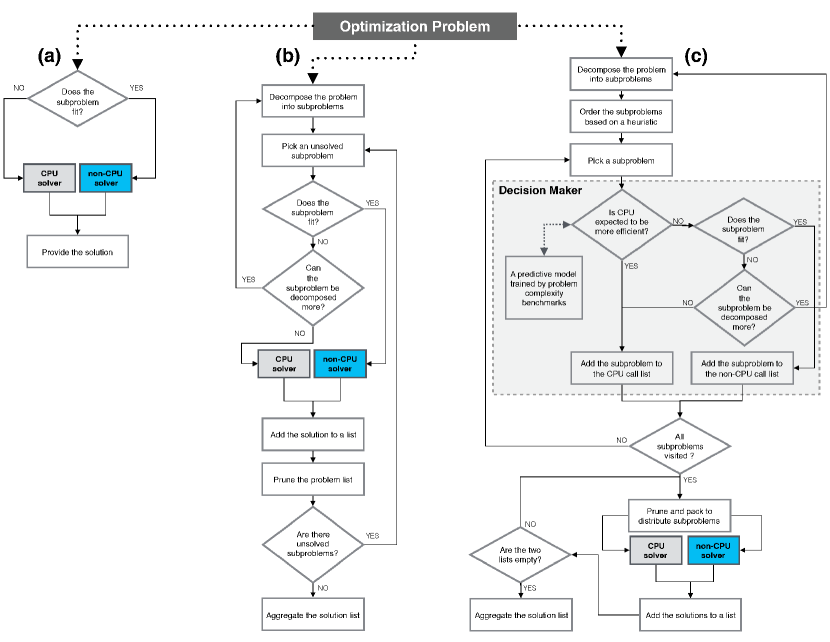
Fig. 1 illustrates three different hybrid approaches to using a CPU-based and a non-CPU-based solver to solve an optimization problem. Flowchart (a) represents the simplest hybrid method, which has the lowest level of sophistication in distributing tasks between the two hardware devices. It solves the problem at hand using the non-CPU solver only if the size of the problem is less than or equal to the size of the solver. In this approach, all problems are meant to be solved using the non-CPU device unless they do not fit on the hardware for some technical reason. The CPU’s function is to carry the pre- and post-processing tasks as well as to solve the problems that do not fit on the non-CPU hardware. Flowchart (b) adds a level of sophistication in that it involves decomposing every subproblem until it either fits the non-CPU hardware, or proves to be difficult to decompose further, in which case it uses a CPU to solve the problem. Finally, the method we propose is depicted in (c). It is a hybrid system that uses the idea of problem decomposition in (b), but augments it with a decision maker and a method that assigns optimization bounds to each subproblem. These additional steps are necessary for the practical use of decomposition techniques in hybrid architectures.

However, as we will demonstrate, not every method of decomposition will be beneficial in a hybrid CPU/non-CPU architecture. For this method to work best in such a scenario, we propose the following requirements:

• the number of generated subproblems should remain a polynomial function of the input;

• the CPU time for finding subproblems should scale polynomially with the input size.

Given these two conditions, the total time spent on solving a problem will remain tractable if the new hardware is capable of efficiently solving problems of a specific type. More precisely, the total computation time in a hybrid architecture can be broken into three components:

$$T_{\text{total}}=t_{\text{CPU}}+t_{\text{comm}}+t_{\text{non-CPU}}.$$ (1)

Here, $t_{\text{CPU}}$ is the total time spent using the CPU. It consists of decomposing the original problem, solving a fraction of the subproblems that are not well-suited for the non-CPU hardware, and converting the remaining subproblems into an acceptable input format for the new hardware (e.g., a QUBO formulation for a device like the D-Wave 2000Q or Fujitsu’s digital annealer). The amount of time devoted to the communication between a CPU and the new hardware is denoted by $t_{\text{comm}}$. This time is proportional to the number of calls made from the CPU to the hardware (which, in itself, is less than the total number of subproblems, as we will explain shortly). Furthermore, $t_{\text{non-CPU}}$ is the total time that it takes for the non-CPU hardware to solve all of the subproblems that it receives.

Given the two requirements for problem decomposition, $t_{\text{CPU}}+t_{\text{comm}}$ remains polynomial, and using the hybrid architecture will be justified if the non-CPU hardware is capable of solving the assigned problems significantly more efficiently than a CPU.

2.1 Problem Decomposition in a Hybrid Architecture

Algorithm 1 comprises our proposed procedure for using problem decomposition in a hybrid architecture. This algorithm takes a $problem$ of size $N$, the size of the non-CPU hardware $nonCPU\_size$, and the maximum number of times to apply the decomposition method decomposition_level as input arguments. In this pseudocode, solve_CPU(.) and solve_nonCPU(.) denote subroutines that solve problems on classical and non-CPU hardware, respectively.

At the beginning, the algorithm checks whether a given $problem$ is “well-suited” for the non-CPU hardware. We define a “well-suited” problem for a non-CPU hardware device as a problem that is expected to be solved faster on a non-CPU device compared to a CPU. This step is performed by the “decision maker” (explained in Sec. 2.2).

The algorithm then proceeds to decompose the problem only if the entire $problem$ is not well-suited for the non-CPU hardware. When a problem is sent to the do_decompose(.) method, it is broken into smaller-sized subproblems, and each subproblem is tagged with an upper bound, in the case of maximization, or a lower bound, in that of minimization. These bounds will be used later to reduce the number of calls to the non-CPU hardware. This decomposition step can be performed a single time, or iteratively up to $decomposition\_level$ times.

After the original problem is decomposed, every new problem in the $subProblem$ list is checked by the decision maker. The well-suited problems are stored in $nonCPU\_subproblems$, and the rest are placed in the $CPU\_subproblems$ list. After the full decomposition has bee achieved, the problems in $nonCPU\_subproblems$ are sent to the PruneAndPack(.) subroutine. This subroutine ignores the problems with an upper bound (lower bound) less than (greater than) the best found solution by the solve_CPU(.) and solve_nonCPU(.) methods, and continues to pack in the rest of the subproblems until the size of the non-CPU hardware has been maxed out. These are necessary steps for minimizing the number of calls to the non-CPU hardware, and thus minimizing the communication time. At the final step, the results of all of the solved subproblems are combined and analyzed using the Aggregate(.) subroutine.

Algorithm 1   Problem Decomposition Algorithm

1:procedure Decompose($problem$, $nonCPU\_size$, $decomposition\_level$)

2:     if $problem$ is not well-suited  then

3:         return Solve_CPU($problem$)      

4:     if $problem\_size<nonCPU\_size$ then

5:         return Solve_nonCPU($problem$)      

6:     $subproblems\leftarrow$ Do_decompose($problem$)

7:     $CPU\_subproblems\leftarrow\emptyset$

8:     $nonCPU\_subproblems\leftarrow\emptyset$

9:     for $problem_{i}$ in $subproblems$ do

10:         if $problem_{i}$ is not well-suited then

11:              $CPU\_subproblems\leftarrow CPU\_subproblems\cup problem_{i}$

12:         else

13:              if $problem\_size>nonCPU\_size$ then

14:                  $level\leftarrow 0$

15:                  $buffer\_list\leftarrow problem$

16:                  while $buffer\_list\_size\neq 0$ and $level<decomposition\_level$ do

17:                       for $p$ in $buffer\_list$ do

18:                           $new\_buffer\_list\leftarrow$ Do_decompose($p$)                        

19:                       $buffer\_list\leftarrow\emptyset$

20:                       for $p$ in $new\_buffer\_list$ do

21:                           if $p$ is not well-suited then

22:                                $CPU\_subproblems\leftarrow CPU\_subproblems\cup p$

23:                           else

24:                                if $p\_size>nonCPU\_size$ then

25:                                    $buffer\_list\leftarrow buffer\_list\cup p$

26:                                else

27:                                    $nonCPU\_subproblems\leftarrow nonCPU\_subproblems\cup p$                                                                                   

28:                       $level\leftarrow level+1$                   

29:              else

30:                  $nonCPU\_subproblems\leftarrow nonCPU\_subproblems\cup problem_{i}$                             

31:     for $p$ in $CPU\_subproblems$ do

32:         $CPU\_result\leftarrow$ Solve_CPU($p$)      

33:     while $nonCPU\_problems$ is not empty do

34:         $packed\_problems\leftarrow$ PruneAndPack($nonCPU\_problems$)

35:         $nonCPU\_result\leftarrow$ Solve_nonCPU($packed\_problems$)      

36:     return Aggregate($nonCPU\_result,cpu\_result$)

2.2 Decision Maker

There is always an overhead cost in converting each subproblem into an acceptable format for the non-CPU hardware, sending the correctly formatted subproblems to this hardware, and finally receiving the answers. It is hence logical to send the subproblems to a “decision maker” before preparing them for the new hardware. In an ideal scenario, this decision maker will have access to a portfolio of classical algorithms, along with the specifications of the non-CPU hardware. Based on this information, the decision maker will be able to decide whether a given problem is well-suited for the non-CPU hardware. These decisions may be achieved via either some simple characteristics of the problem, or through intelligent machine-learning models with good predictive power, depending on the case at hand.

3 Specific Case Study: Maximum Clique

Now that we have laid out the specifics of our proposal for problem decomposition in a hybrid architecture, we apply this method to the maximum clique problem. We begin by explaining the graph theory notation and necessary definitions, along with a few real-world applications for the maximum clique problem.

A graph $G=(V,E)$ consists of a finite set $V=\{v_{1},v_{2},\ldots,v_{n}\}$ of vertices and a set $E\subseteq V\times V$ of edges. Two distinct vertices $v_{i}$ and $v_{j}$ are adjacent if $\{v_{i},v_{j}\}\in E$. The neighbourhood of a vertex $v$ is denoted by $\mathcal{N}(v)$, and is the subset of vertices of $G$ which are adjacent to $v$. The degree of a vertex $v$ is the cardinality of $\mathcal{N}(v)$, and is denoted by $d(v)$. The maximum degree and minimum degree of a graph are denoted by $\Delta(G)$ and $\delta(G)$, respectively.

The subgraph of $G$ induced by a subset of vertices $U\subseteq V$ is denoted by $G[U]$ and consists of the vertex set $U$, and the edge set defined by

$$E(G[U])=\{\{u_{i},u_{j}\}~{}|~{}u_{i},~{}u_{j}\in U,~{}\{u_{i},u_{j}\}\in E(G)\}.$$

A complete subgraph, or a clique, of $G$ is a subgraph of $G$ where every pair of its vertices are adjacent. The size of a maximum clique in a graph $G$ is called the clique number of $G$ and is denoted by $\omega(G)$. An independent set of $G$, on the other hand, is a set of pairwise nonadjacent vertices. As every clique of a graph is an independent set of the complement graph, one can find a maximum independent set of a graph by simply solving the maximum clique problem in its complement.

A node-weighted graph $G$ is a graph that is augmented with a set of positive weights $W=\{w_{1},w_{2},\ldots,w_{n}\}$ assigned to each node. The maximum weighted-clique problem is the task of finding a clique with the largest sum of weights on its nodes.

Many real-world applications have been proposed in the literature for the maximum clique and maximum independent set problems. One commonly suggested application is community detection for social network analysis [20]. Even though cliques are known to be too restrictive for finding communities in a network, they prove to be useful in finding overlapping communities. Another example is the finding of the largest set of correlated/uncorrelated instruments in financial markets. This problem can be readily modelled as a maximum clique problem, and it plays an important role in risk management and the design of diversified portfolios (see [21] and [22]). Recent studies have shown some merit in using a weighted maximum-clique finder for drug discovery purposes (see [23] and [24]). In these studies, the structures of molecules are stored as graphs, and the properties of unknown molecules are predicted by solving the maximum common subgraph problem using the graph representations of the molecules. Aside from the proposed industrial applications, the clique problem is one of the better-studied NP-hard problems, and there exist powerful heuristic and exact algorithms for solving the maximum clique problem in the literature (see, e.g., [13], [25], and [26]). It is, therefore, beneficial to map a part of, or an entire, optimization problem into a clique problem and benefit from the runtime of these algorithms (see, e.g., [27]).

4 Problem Decomposition for the Maximum Clique Problem

In this section, we explain the details of two problem decomposition methods for the maximum clique problem. The first approach is based on the branch-and-bound framework and is similar to what is dubbed “vertex splitting” in Ref. [28]. This method is briefly explained in Sec. 4.1, followed by a discussion on why it fails to meet the problem decomposition requirements of Sec. 2. We then present our own method in Sec. 4.2 and prove that it is an effective problem decomposition method, that is, it generates a polynomial number of subproblems and requires polynomial computational complexity to generate each subproblem.

4.1 Branch and Bound

The branch-and-bound technique (BnB) is a commonly used method in exact algorithms for solving the maximum clique problem (see Ref. [13] for a comprehensive review on the subject). At a very high level, BnB consists of three main procedures that are repeatedly applied to a subgraph of the entire graph until the size of the maximum clique is found. The main procedures of a BnB approach consist of: (a) ordering the vertices in a given subproblem and adding the highest-priority vertex to the solution list; (b) finding the space of feasible solutions based on the vertices in the solution list; and (c) assigning upper bounds to each subproblem.

Figure 2: Abstract illustration of a branch-and-bound search tree

Fig. 2 shows a schematic representation of the steps involved in traversing the BnB search tree. In the first step, all of the vertices of the graph are listed at the root of the tree, representing the space of feasible solutions, along with an empty set that will contain possible solutions as the algorithm traverses the search tree (we will call this set “growing-clique”). The vertices inside the feasible space are ordered based on some criteria (e.g., increasing/decreasing degree, or the sum of the degree of the neighbours of a vertex [29]), and the highest-priority vertex ($v_{\rm 1}$) is chosen as the “branching node”. The branching node is added to growing-clique and the neighbourhood of this node ($\mathcal{N}(v_{\rm 1})$) is chosen as the new space of feasible solutions. This procedure continues until the domain of feasible solutions becomes an empty list, indicating that growing-clique now contains a maximal clique. If the size of this clique is larger than the best existing solution, the best solution is updated. The number of nodes in the BnB tree is greatly reduced by applying some upper bounds based on graph colouring [30] or Max-SAT reasoning [31]. These upper bounds prune the tree if the upper bound on the size of the clique inside a feasible space is smaller than the best found solution (minus the size of growing-clique).

In a fully classical approach, the entire BnB search tree is explored via a classical computer. On the other hand, some of the work can be offloaded to the non-conventional hardware in the hybrid scenario. More precisely, one can stop traversing a particular branch of the search tree when the size of the subproblem under consideration becomes smaller than the capacity of the non-conventional hardware (see, e.g., [28]). Although this idea can combine the two hardware devices in an elegant and coherent way, it suffers from two main drawbacks. It creates an exponential number of subproblems (see Fig. $6$ in Ref. [28]), and, in the worst case, it takes an exponential amount of time to traverse the search tree until the size of the subproblem becomes smaller than the capacity of the non-conventional hardware.

4.2 A Proposed Method for Problem Decomposition

Algorithm 2   $k$-Core Computation and Degeneracy Ordering

1:procedure K-Core_Compute(undirected weighted graph $G=(V,E)$)

2:     $sorted\_nodes$ $\leftarrow$ an empty list

3:     for  every $v\in G$ do

4:         $K(v)\leftarrow d(v)$      

5:     $V^{\prime}\leftarrow$ order vertex set $V$ by non-decreasing vertex degree

6:     while $V^{\prime}$ is not empty do

7:         select a vertex $v$ with minimum $k$-core, and find its neighbourhood $\mathcal{N}(v)$

8:         for  every $u\in\mathcal{N}(v)$ do

9:              if $K(u)>K(v)$ then

10:                  $K(u)\leftarrow K(u)-1$                        

11:         $sorted\_nodes\leftarrow sorted\_nodes\cup\{v\}$

12:         $V^{\prime}\leftarrow V^{\prime}\setminus\{v\}$      

13:     return $sorted\_nodes$, $k$-$core$

In this section, we explain our proposed problem decomposition method, which is much more effective than BnB (explained in the previous section). We show, in particular, that our proposed method generates a much smaller number of subproblems compared to BnB, and that these subproblems can be obtained via an efficient $\mathcal{O}(E)$ algorithm.

Our method begins by sorting the vertices of the graph based on their $k$-core number. Ref. [32] details the formal $k$-core definition, and proposes an efficient $\mathcal{O}(E)$ algorithm for calculating the $k$-core number of the vertices of a graph. Intuitively, the $k$-core number of a vertex $v$ is equal to $k$ if it has at least $k$ neighbours of a degree higher than or equal to $k$, and not more than $k$ neighbours of a degree higher than or equal to $k+1$. We denote the core number of a vertex $v$ by $K(v)$.

The core number of a graph $G$, denoted by $K(G)$, is the highest-order core of its vertices. $K(G)$ is always upper bounded by the maximum degree of the vertices of the graph $\Delta(G)$, and the minimum core number of the vertices is always equal to the minimum degree $\delta(G)$. A degeneracy, or k-core ordering, of the vertices of a graph $G$ is a non-decreasing ordering of the vertices of $G$ based on their core numbers. Algorithm 2 is a method for finding the $k$-core ordering of the vertices along with their $k$-core numbers. The following proposition shows that, given a degeneracy ordering for the vertices of the graph, one can decompose the maximum clique problem into a linear number of subproblems. Our proposed method is based on this proposition.

Proposition 1.

For a graph $G$ of size $n$, one can decompose the maximum clique problem in $G$ into at most $n-K(G)+1$ subproblems, each of which is upper-bounded in size by $K(G)$.

Proof.

Let $d(v)$ be the degree of vertex $v$ in $G$. From Algorithm 2 (lines $8$–$11$), the number of vertices that are adjacent to $v$ and precede vertex $v$ in $sorted\_nodes$ is greater than or equal to $d(v)-K(v)$. Therefore, the number of vertices that appear after $v$ in this ordering is upper-bounded by $K(v)$. Using this fact, the algorithm starts from the last $K(G)$ vertices of $sorted\_node$, and solves the maximum clique on that induced subgraph. It then moves towards the beginning of $sorted\_node$ vertex by vertex. Each time it takes a root vertex $w$ and forms a new subproblem by finding the adjacent vertices that are listed after $w$ in $sorted\_node$. The size of these subproblems is upper-bounded by $K(w)$, which itself is upper-bounded by $K(G)$, and the number of the subproblems created in this way is exactly $n-K(G)+1$.

Since we have

$$\omega(G)\leq K(G)+1\leq\Delta(G)+1,$$

one can stop the procedure as soon as the size of the clique becomes larger than or equal to the $k$-core number of a root vertex. ∎

To illustrate, consider the 6-cycle with a chord shown in Fig. 3. In the first step, the vertices are ordered based on their core numbers, according to Algorithm 2: $sorted\_nodes$ = [c, b, e, f, d, a].

Figure 3: A 6-cycle graph with a chord

Following our proposed algorithm, we first consider the subgraph induced by the last $K(G)=2$ vertices from the list, that is, $[a,d]$. Solving the maximum clique problem in this subgraph results in a lower bound on the size of the maximum clique, that is, $\omega(G)\geq 2$. After this step, we proceed by considering the vertices one by one from the end of $sorted\_nodes$ to form the subproblems that follow:

$$root\_node\quad subproblem$$

$$f\qquad\quad\, \quad\quad\{\}$$

$$e\qquad\quad\, \quad\,\,\{f,d\}$$

$$b\qquad\quad\, \quad\,\,\,\,\,\{a\}$$

$$c\qquad\quad\, \quad\,\,\{b,d\}\,.$$

Among these subproblems, only the two with $root\_node=\{e,c\}$ need to be examined by the clique solver, since the size of the other subproblems is less than or equal to the size of the largest clique found. This example shows how a problem of size six can be broken down to three problems of size two.

As a final note, the $k$-core decomposition takes $\mathcal{O}(E)$ time, and constructing the resulting subproblems takes $\mathcal{O}(N^{2})$. The entire process takes $\mathcal{O}(E+N^{2})$ time at the first level, and $\mathcal{O}(N^{(\ell+1)})$ time at $decomposition\_level=\ell$. The maximum number of subproblems can grow up to $N^{\ell}$ at $decomposition\_level=\ell$.

5 Results

In this section, we discuss our numerical results for different scenarios in terms of density and the size of the underlying graph. In particular, we study the effect of the graph core number, $K(G)$, and the density of the graph on the number of generated subproblems. In the fully classical approach, we also compare the running time of our proposed algorithm with state-of-the-art methods for solving the maximum clique problem in the large, sparse graphs. It is worth noting that $k$-core decomposition is widely used in exact maximum clique solvers as a means to find computationally inexpensive and relatively tight upper bounds in large, sparse graphs. However, to the best of our knowledge, no one has used $k$-core decomposition as a method of problem decomposition as is proposed in this paper (e.g., Ref. [28] uses it for pruning purposes and BnB for decomposition).

5.1 Large and Sparse Graphs

The importance of Proposition 1 is more pronounced when we consider the standard large, sparse graphs listed in Table I. For each of these graphs, we first perform one round of $k$-core decomposition, and then solve the generated subproblems with our own exact maximum clique solver. It is worth mentioning that, after decomposing the original problem into sufficiently smaller subproblems, our approach for finding the maximum clique of the smaller subproblems is similar to what has been proposed in Ref. [33].

TABLE I: The number of subproblems and the runtime results (in seconds) for exact maximum clique solvers (1QBit’s solver, PMC, and BBMCSP) on network graphs from the Stanford Large Network Dataset Collection [34] and Network Repository [35]. “MaxClique” refers to the size of the maximum clique. All three codes are implemented in C++ and run on an Ubuntu machine with 32 GB of memory and an Intel 3.60 GHz processor.

						Runtime (s)
Graph Name	Num. of Vertices	Num. of Edges	$K(G)$	MaxClique	1QBit Solver	PMC	BBMCSP	Num. of Subprobs.
Stanford Large Network
Dataset:
ego-Facebook	$4,039$	$88,234$	$115$	$69$	0.009	$0.04$	$0.03$	$367$
ca-CondMat	$23,133$	$93,468$	$25$	$26$	0.004	$0.03$	$0.02$	$3$
email-Enron	$36,692$	$25,985$	$43$	$20$	0.01	$0.3$	$0.06$	$2235$
com-Amazon	$334,863$	$925,872$	$6$	$7$	0.06	$0.06$	$0.2$	$3$
roadNet-PA	$1,088,092$	$1,541,898$	$3$	$4$	0.1	$2.1$	$0.4$	$580$
com-Youtube	$1,134,890$	$2,987,624$	$51$	$17$	0.5	$2.0$	$2.5$	$24466$
as-skitter	$1,696,415$	$11,095,298$	$111$	$67$	0.7	$1.4$	$5.6$	$4087$
roadNet-CA	$1,965,206$	$2,766,607$	$3$	$4$	0.2	$3.9$	$0.4$	$2286$
com-Orkut	$3,072,441$	$117,185,083$	$253$	$51$	82	$179$	$220$	$741349$
com-LiveJournal	$3,997,962$	$34,681,189$	$360$	$327$	2.1	$2.5$	$20$	$25$
Network Repository Graphs:
soc-buzznet	$101,163$	$2,763,066$	$153$	$31$	1.9	$14.6$	$4.0$	$29484$
soc-catster	$149,700$	$5,448,197$	$419$	$81$	1.1	$>1\mathrm{\,h}$	$5.5$	$12095$
delaunay-n20	$1,048,576$	$3,145,686$	$4$	$4$	1.4	$2.5$	$2.8$	$1036595$
web-wikipedia-growth	$1,870,709$	$36,532,531$	$206$	$31$	18	$397$	file not supported	$358272$
delaunay-n21	$2,097,152$	$6,291,408$	$4$	$4$	2.8	$5.1$	2.8	$2073021$
tech-ip	$2,250,498$	$21,643,497$	$253$	$4$	28	$1031$	$220$	$222338$
soc-orkut-dir	$3,072,441$	$117,185,083$	$253$	$51$	74	$188$	$170$	$741349$
socfb-A-anon	$3,097,165$	$23,667,394$	$74$	$25$	10	$18$	$30$	$357836$
soc-livejournal-user-groups	$7,489,073$	$112,305,407$	$116$	$9$	103	$>1\mathrm{\,h}$	$1600$	$2404573$
aff-orkut-user2groups	$8,730,857$	$327,036,486$	$471$	$6$	852	$>1\mathrm{\,h}$	$2400$	$4173108$
soc-sinaweibo	$58,655,849$	$261,321,033$	$193$	$44$	93	$>1\mathrm{\,h}$	$1070$	$713652$

In the large and sparse regime, the core numbers of the graphs are typically orders of magnitude smaller than the number of vertices in the graph. This implies that non-CPU hardware of a size substantially smaller than the size of the original problem can be used to find the maximum clique of these massive graphs. For example, the com-Amazon graph, with 334,863 vertices and 925,872 edges has $K(G)=6$. These facts, combined with Proposition 1, imply that this graph can be decomposed into $\sim$ 334,863 problems of a size $\leq 6$. However, as the table shows, the actual number of subproblems that should be solved is only three, since the $k$-core number of the next subproblem drops to a number less than or equal to the size of the largest clique that was found. Hence, in this specific case, a single call to a non-CPU hardware device of size greater than $21$ can solve the entire problem, that is, this problem can be solved by submitting an effective problem of size 21 to the D-Wave 2000Q chip.

Numerical results also indicate that the fully classical runtime of our proposed method is considerably faster than two of the best-known algorithms in the literature for large–sparse graphs, namely PMC [33] and BBMCSP [36]. Table I shows that in some instances, our method is orders of magnitude faster than these algorithms.

5.2 Hierarchy of minimum degree, maximum degree, max $k$-core, and clique number

The $k$-core decomposition proves extremely powerful in the large and sparse regime because it dramatically reduces the size of the problem, and also prunes a good number of the subproblems. This situation changes as we move towards denser and denser graphs. As graphs increase in density, $K(G)$ approaches the graph size, and the size reduction becomes less effective in a single iteration of decomposition. It is hence necessary to apply the decomposition method for at least a few iterations in the dense regime.

Figure 4: $\omega(G)$, $K(G)$, $\Delta(G)$, and $\delta(G)$ comparisons in different graph density regimes

Moreover, the number of subproblems that should be solved also grows as the graphs increase in density. This is partially due to there being more rounds of decomposition, and partially to the hierarchy of the clique number $\omega(G)$ and the maximum and minimum core numbers (shown in Fig. 4). In the sparse regime, the clique number $\omega(G)$ lies between the minimum core number $\delta(G)$ and the core number of the graph $K(G)$. This means that all of the subproblems that stem from a root node with a core number less than the clique number can be pruned. This phenomenon leads to the effective pruning that is reflected in the number of subproblems listed in Table I. On the other hand, as shown in Fig. 4, the minimum core of the graph, i.e, $\delta(G)$ is larger than the clique number in the dense regime. Therefore, core numbers are no longer suitable for upper-bounding purposes, and some other upper-bounding methods should be used, as we discuss in the next section.

5.3 Dense Graphs

As explained in the previous section, the $k$-core number becomes an ineffective upper bound in the case of dense graphs; therefore, the number of subproblems that should be solved grows as $N^{\ell}$ for $\ell$ levels of decomposition. Because of this issue, and since colouring is an effective upper bound in the dense regime, we used the heuristic DSATUR algorithm explained in Ref. [14] to find the colour numbers of each generated subproblem. We then ignored the subproblems with a colour number less than the size of the largest clique that has been found from the previous set of subproblems. This technique reduces the number of subproblems by a large factor, as can be seen in Table II. In this table, we present the results for random Erdős–Rényi graphs of three different sizes and varying densities. For each size and density, we generated $10$ samples, and decomposed the problems iteratively three levels ($decomposition\_level=3$). The reported results are the average of the $10$ samples for each category. “max”, “min”, and “avg” refer to the maximum, minimum, and average size of the generated subproblems at every level.

TABLE II: Problem decomposition statistics for the maximum clique of random Erdős–Rényi graphs of different sizes and densities. The first number in parentheses represents size, and the second number is the edge presence probability (which ends up being the graph density to a desired level of precision).

				Level 1				Level 2				Level 3
Graph Name	$K(G)$	MaxClique	Num. of Subprobs.	max	min	avg	Num. of Subprobs.	max	min	avg	Num. of Subprobs.	max	min	avg
ER(200,0.3)	$47.7$	$7.2$	$153.3$	$48$	$16$	$36$	$74$	$13$	$8$	$10$	14.1	5	2	5
ER(200,0.4)	$66.2$	$9$	$134.8$	$66$	$27$	$52$	$460$	$26$	$12$	$19$	5.4	9	6	8
ER(200,0.5)	$85.3$	$11$	$115.7$	$85$	$44$	$69$	$2941.2$	$42$	$17$	$29$	418.7	21	12	16
ER(200,0.6)	$104.2$	$13.9$	$96.8$	$104$	$62$	$88$	$3856.6$	$60$	$26$	$43$	6685.3	37	18	26
ER(500,0.3)	$127.8$	$8.5$	$373.2$	$128$	$38$	$93$	$8364.4$	$37$	$12$	$25$	217.2	10	6	7
ER(500,0.4)	$174.8$	$10.3$	$326.2$	$175$	$71$	$133$	$23813.6$	$67$	$18$	$42$	11050.9	28	11	18
ER(500,0.5)	$223.1$	$13$	$277.9$	$223$	$113$	$177$	$27437.3$	$107$	$29$	$67$	359735	54	17	33
ER(1000,0.1)	$80.8$	$5.4$	$920.2$	$81$	$7$	$54$	$985.1$	$7$	$4$	$7$	658.9	5	4	4
ER(1000,0.2)	$171.9$	$7.2$	$829.1$	$172$	$33$	$116$	$15666.3$	$33$	$8$	$22$	361	8	6	6
ER(1000,0.3)	$265.6$	$9.1$	$735.4$	$266$	$78$	$188$	$82170.8$	$76$	$15$	$44$	13515.9	24	8	15

Notice the significant difference in the $\frac{K(G)}{\rm{graph\,size}}$ ratio between the sparse graphs presented in Table I and the relatively dense graphs presented here. Unlike in the sparse regime, the gain in size reduction after one level of decomposition is only a factor of few. This means that a graph of size $N$ is decomposed into $\sim N$ graphs of smaller but relatively similar size after one level of decomposition. This fact hints towards using more levels of decomposition, as with more decomposition, the maximum size of the subproblems decreases. However, there is usually a tradeoff between the number of generated subproblems and the maximum size of these subproblems, as can be seen in Table II. It is, therefore, not economical to use problem decomposition for these types of graphs in a fully classical approach for solving the maximum clique problem in dense graphs. However, if a specialized non-CPU hardware device becomes significantly faster than the performance of CPUs on the original problem, this problem decomposition approach will become useful. In fact, the merit of this approach compared to the BnB-based decomposition, shown in Fig. 6 in Ref. [28], is that it generates considerably fewer of subproblems, and that the time for constructing the subproblems is polynomial.

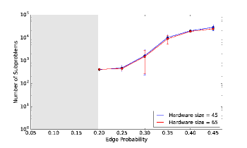
Fig. 5 shows the scaling of the number of subproblems with the density of the graph. For this plot, we assume two devices of size $\{45,65\}$, representing an instance of the D-Wave 2X chip, and the theoretical upper bound on the maximum size of a complete graph embeddable into the new D-Wave 2000Q chip. The graph size is fixed to 500 in every case, and the points are the average of 10 samples, with error bars showing standard deviation. For each point, we first run a heuristic on the whole graph, and then prune the subproblems based on their colour numbers obtained using the DSATUR algorithm of Ref. [14]. Densities below 0.2 are shaded with a grey band, since the number of subproblems for $\{0.05,0.1,0.15\}$ densities is zero. This happens because all of the subproblems are pruned after the second round of decomposition. Aside from scaling with respect to density, this plot also shows that a small increase to the size of the non-CPU hardware (e.g., from 45 nodes to 65), will not have a significant effect on the total number of generated subproblems. In these scenarios, the non-CPU hardware becomes competitive with classical CPUs only if, in comparison to CPUs, it can either solve a single problem with very high quality and speed, or it can be mass produced and parallelized at lower costs.

Figure 5: Scaling of the number of subproblems with density. Graph size is fixed to 500 in every case, and every point is the average of 10 samples, with error bars representing sample standard deviation.

6 Discussion

We focused on the specific case of the maximum clique problem and proposed a method of decomposition for this problem. Our proposed decomposition technique is based on the $k$-core decomposition of the input graph. The approach is motivated mostly by the emergence of non-CPU hardware for solving hard problems. This approach is meant to extend the capabilities of this new hardware for finding the maximum clique of large graphs. While the size of generated subproblems is greatly reduced in the case of sparse graphs after a single level of decomposition, an effective size reduction happens only after multiple levels of decomposition in the dense regime. Compared to the branch-and-bound method, this method generates considerably fewer subproblems, and creates these subproblems in polynomial time.

We believe that further research on finding tighter upper bounds on the size of the maximum clique in each subproblem would be extremely useful. Tighter upper bounds make it possible to attain more levels of decomposition, and hence reduce the problem size, without generating too many subproblems.

In the fully classical approach, there is a chance that combining integer programming solvers for the maximum clique problem with our proposed method can lead to better runtimes for dense graphs, or for large, sparse graphs with highly dense $k$-cores. This suggestion is based on from the fact that integer programming solvers such as CPLEX become highly competitive for graphs of moderate size, that is, between 200 and 2000, and high density, that is, higher than 90% (e.g., see Table 1 in Ref. [37]). Since $k$-core decomposition tends to generate relatively high-density and small-sized subgraphs, the combination of the two we consider to be a promising avenue for future study.

References

- [1] J. Błażewicz, K. H. Ecker, E. Pesch, G. Schmidt, and J. Weglarz, Scheduling computer and manufacturing processes. Springer Science & Business Media, 2013.
- [2] P. Kouvelis and G. Yu, Robust discrete optimization and its applications. Springer Science & Business Media, 2013, vol. 14.
- [3] A. Kasirzadeh, M. Saddoune, and F. Soumis, “Airline crew scheduling: models, algorithms, and data sets,” EURO Journal on Transportation and Logistics, vol. 6, no. 2, pp. 111–137, 2017.
- [4] C. Holland, J. Levis, R. Nuggehalli, B. Santilli, and J. Winters, “UPS optimizes delivery routes,” Interfaces, vol. 47, no. 1, pp. 8–23, 2017. [Online]. Available: https://doi.org/10.1287/inte.2016.0875
- [5] V. N. Smelyanskiy, E. G. Rieffel, S. I. Knysh, C. P. Williams, M. W. Johnson, M. C. Thom, W. G. Macready, and K. L. Pudenz, “A Near-Term Quantum Computing Approach for Hard Computational Problems in Space Exploration,” ArXiv e-prints, Apr. 2012.
- [6] G. Rosenberg, P. Haghnegahdar, P. Goddard, P. Carr, K. Wu, and M. L. de Prado, “Solving the optimal trading trajectory problem using a quantum annealer,” IEEE Journal of Selected Topics in Signal Processing, vol. 10, no. 6, pp. 1053–1060, 2016.
- [7] D. Venturelli, D. J. Marchand, and G. Rojo, “Quantum annealing implementation of job-shop scheduling,” arXiv preprint arXiv:1506.08479, 2015.
- [8] R. Dridi and H. Alghassi, “Prime factorization using quantum annealing and computational algebraic geometry,” Scientific Reports, vol. 7, p. 43048, 2017.
- [9] M. Hernandez, A. Zaribafiyan, M. Aramon, and M. Naghibi, “A novel graph-based approach for determining molecular similarity,” arXiv preprint arXiv:1601.06693, 2016.
- [10] V. Mak-Hau, “On the kidney exchange problem: Cardinality constrained cycle and chain problems on directed graphs: A survey of integer programming approaches,” J. Comb. Optim., vol. 33, no. 1, pp. 35–59, Jan. 2017. [Online]. Available: https://doi.org/10.1007/s10878-015-9932-4
- [11] C. Moore and S. Mertens, The Nature of Computation. New York, NY, USA: Oxford University Press, Inc., 2011.
- [12] P. San Segundo, A. Lopez, and P. M. Pardalos, “A new exact maximum clique algorithm for large and massive sparse graphs,” Computers & Operations Research, vol. 66, pp. 81–94, 2016.
- [13] P. Prosser, “Exact Algorithms for Maximum Clique: a computational study,” ArXiv e-prints, Jul. 2012.
- [14] R. Lewis, A Guide to Graph Colouring. Springer, 2015.
- [15] M. W. Johnson, M. H. S. Amin, S. Gildert, T. Lanting, F. Hamze, N. Dickson, R. Harris, A. J. Berkley, J. Johansson, P. Bunyk, E. M. Chapple, C. Enderud, J. P. Hilton, K. Karimi, E. Ladizinsky, N. Ladizinsky, T. Oh, I. Perminov, C. Rich, M. C. Thom, E. Tolkacheva, C. J. S. Truncik, S. Uchaikin, J. Wang, B. Wilson, and G. Rose, “Quantum annealing with manufactured spins,” Nature, vol. 473, no. 7346, pp. 194–198, May 2011. [Online]. Available: http://dx.doi.org/10.1038/nature10012
- [16] F. L. Ltd., “Fujitsu laboratories develops new architecture that rivals quantum computers in utility,” 2016.
- [17] C. C. McGeoch, “Adiabatic quantum computation and quantum annealing: Theory and practice,” Synthesis Lectures on Quantum Computing, vol. 5, no. 2, pp. 1–93, 2014.
- [18] T. T. Tran, M. Do, E. G. Rieffel, J. Frank, Z. Wang, B. O’Gorman, D. Venturelli, and J. C. Beck, “A hybrid quantum-classical approach to solving scheduling problems,” in Proceedings of the Ninth Annual Symposium on Combinatorial Search, SOCS 2016, Tarrytown, NY, USA, July 6-8, 2016., J. A. Baier and A. Botea, Eds. AAAI Press, 2016, pp. 98–106. [Online]. Available: http://aaai.org/ocs/index.php/SOCS/SOCS16/paper/view/13958
- [19] M. Booth, S. Reinhardt, and A. Roy, “Partitioning optimization problems for hybrid classical/quantum execution,” dWave Technical Report.
- [20] S. Fortunato, “Community detection in graphs,” Physics Reports, vol. 486, pp. 75–174, Feb. 2010.
- [21] V. Boginski, S. Butenko, and P. M. Pardalos, “Statistical analysis of financial networks.” Computational Statistics & Data Analysis, vol. 48, no. 2, pp. 431–443, 2005. [Online]. Available: http://dblp.uni-trier.de/db/journals/csda/csda48.html#BoginskiBP05
- [22] F. Cesarone, A. Scozzari, and F. Tardella, “A new method for mean-variance portfolio optimization with cardinality constraints,” Annals of Operations Research, vol. 205, no. 1, pp. 213–234, 05 2013.
- [23] S. Butenko and W. Wilhelm, “Clique-detection models in computational biochemistry and genomics,” European Journal of Operational Research, vol. 173, no. 1, pp. 1 – 17, 2006. [Online]. Available: http://www.sciencedirect.com/science/article/pii/S0377221705005266
- [24] M. Hernandez, A. Zaribafiyan, M. Aramon, and M. Naghibi, “A novel graph-based approach for determining molecular similarity,” CoRR, vol. abs/1601.06693, 2016. [Online]. Available: http://arxiv.org/abs/1601.06693
- [25] Y. Wang, S. Cai, and M. Yin, “Two efficient local search algorithms for maximum weight clique problem,” in Proceedings of the Thirtieth AAAI Conference on Artificial Intelligence, February 12-17, 2016, Phoenix, Arizona, USA., 2016, pp. 805–811. [Online]. Available: http://www.aaai.org/ocs/index.php/AAAI/AAAI16/paper/view/11915
- [26] P. San Segundo, A. Lopez, J. Artieda, and P. M. Pardalos, “A parallel maximum clique algorithm for large and massive sparse graphs,” Optimization Letters, pp. 1–16, 2016. [Online]. Available: http://dx.doi.org/10.1007/s11590-016-1019-3
- [27] Q. Wu and J.-K. Hao, “Solving the winner determination problem via a weighted maximum clique heuristic,” Expert Syst. Appl., vol. 42, no. 1, pp. 355–365, Jan. 2015. [Online]. Available: http://dx.doi.org/10.1016/j.eswa.2014.07.027
- [28] G. Chapuis, H. Djidjev, G. Hahn, and G. Rizk, “Finding maximum cliques on a quantum annealer,” in Proceedings of the Computing Frontiers Conference, ser. CF’17. New York, NY, USA: ACM, 2017, pp. 63–70. [Online]. Available: http://doi.acm.org/10.1145/3075564.3075575
- [29] E. Tomita and T. Kameda, “An efficient branch-and-bound algorithm for finding a maximum clique with computational experiments,” Journal of Global Optimization, vol. 37, no. 1, pp. 95–111, Jan. 2007. [Online]. Available: http://dx.doi.org/10.1007/s10898-006-9039-7
- [30] E. Tomita and T. Seki, “An efficient branch-and-bound algorithm for finding a maximum clique,” in Proceedings of the 4th International Conference on Discrete Mathematics and Theoretical Computer Science, ser. DMTCS’03. Berlin, Heidelberg: Springer-Verlag, 2003, pp. 278–289. [Online]. Available: http://dl.acm.org/citation.cfm?id=1783712.1783736
- [31] C. M. Li and Z. Quan, “An efficient branch-and-bound algorithm based on maxsat for the maximum clique problem.” in AAAI, M. Fox and D. Poole, Eds. AAAI Press, 2010. [Online]. Available: http://dblp.uni-trier.de/db/conf/aaai/aaai2010.html#LiQ10
- [32] V. Batagelj and M. Zaversnik, “An O(m) Algorithm for Cores Decomposition of Networks,” eprint arXiv:cs/0310049, Oct. 2003.
- [33] R. A. Rossi, D. F. Gleich, A. H. Gebremedhin, and M. M. A. Patwary, “Parallel Maximum Clique Algorithms with Applications to Network Analysis and Storage,” ArXiv e-prints, Feb. 2013.
- [34] J. Leskovec and A. Krevl, “SNAP Datasets: Stanford large network dataset collection,” http://snap.stanford.edu/data, Jun. 2014.
- [35] R. A. Rossi and N. K. Ahmed, “The network data repository with interactive graph analytics and visualization,” in Proceedings of the Twenty-Ninth AAAI Conference on Artificial Intelligence, 2015. [Online]. Available: http://networkrepository.com
- [36] P. San Segundo, A. Lopez, and P. M. Pardalos, “A new exact maximum clique algorithm for large and massive sparse graphs,” Comput. Oper. Res., vol. 66, no. C, pp. 81–94, Feb. 2016. [Online]. Available: http://dx.doi.org/10.1016/j.cor.2015.07.013
- [37] Z. Fang, C.-M. Li, and K. Xu, “An exact algorithm based on maxsat reasoning for the maximum weight clique problem,” Journal of Artificial Intelligence Research, vol. 55, pp. 799–833, 2016.