Global dynamics of planar quasi–homogeneous differential systems

Abstract.

In this paper we provide a new method to study global dynamics of planar quasi–homogeneous differential systems. We first prove that all planar quasi–homogeneous polynomial differential systems can be translated into homogeneous differential systems and show that all quintic quasi–homogeneous but non–homogeneous systems can be reduced to four homogeneous ones. Then we present some properties of homogeneous systems, which can be used to discuss the dynamics of quasi–homogeneous systems. Finally we characterize the global topological phase portraits of quintic quasi–homogeneous but non–homogeneous differential systems.

1. Introduction

In the qualitative theory of planar polynomial differential systems, there are lots of results on their global topological structures. But there are only few class of planar polynomial differential systems whose topological phase portraits were completely characterized. This paper will focus on the global structures of quasi–homogeneous polynomial differential systems.

Consider a real planar polynomial differential system

(1) $$\dot{x}=P(x,y),\qquad\qquad\dot{y}=Q(x,y),$$

where $P(x,y),Q(x,y)\in\mathbb{R}[x,y]$, $PQ\not\equiv 0$ and the origin $O=(0,0)$ is a singularity of system (1). As usual, the dot denotes derivative with respect to an independent real variable $t$ and $\mathbb{R}[x,y]$ denotes the ring of polynomials in the variables $x$ and $y$ with coefficients in $\mathbb{R}$. We say that system (1) has degree $n$ if $n=\max\{\mbox{deg}\,P,\mbox{deg}\,Q\}$. In what follows we assume without loss of generality that $P$ and $Q$ in system (1) have not a non–constant common factor.

System (1) is called a quasi–homogeneous polynomial differential system if there exist constants $s_{1},s_{2},d\in\mathbb{N}$ such that for an arbitrary $\alpha\in\mathbb{R}_{+}$ it holds that

(2) $$P(\alpha^{s_{1}}x,\alpha^{s_{2}}y)=\alpha^{s_{1}+d-1}P(x,y),\ \ \ \ Q(\alpha^{s_{1}}x,\alpha^{s_{2}}y)=\alpha^{s_{2}+d-1}Q(x,y),$$

where $\mathbb{N}$ is the set of positive integers and $\mathbb{R}_{+}$ is the set of positive real numbers. We call $(s_{1},s_{2})$ weight exponents of system (1) and $d$ weight degree with respect to the weight exponents. Moreover, $w=(s_{1},s_{2},d)$ is denominated weight vector of system (1) or of its associated vector field. For a quasi–homogeneous polynomial differential system (1), a weight vector $\widetilde{w}=(\widetilde{s}_{1},\widetilde{s}_{2},\tilde{d})$ is minimal for system (1) if any other weight vector $(s_{1},s_{2},d)$ of system (1) satisfies $\tilde{s}_{1}\leq s_{1},\tilde{s}_{2}\leq s_{2}$ and $\tilde{d}\leq d$. Clearly each quasi–homogeneous polynomial differential system has a unique minimal weight vector. When $s_{1}=s_{2}=1$, system (1) is a homogeneous one of degree $d$.

Quasi–homogeneous polynomial differential systems have been intensively investigated by many different authors from integrability point of view, see for example [2, 14, 15, 16] and the references therein. It is well known that all planar quasi–homogeneous vector fields are Liouvillian integrable, see e.g. [11, 12, 17]. Specially, for the polynomial and rational integrability of planar quasi–homogeneous vector fields we refer readers to [3, 6, 20, 28], and for the center and limit cycle problems we refer to [1, 13, 17] and the references therein.

Homogeneous differential systems are a class of special quasi–homogeneous polynomial differential systems of form (1) with $\mbox{deg}\,P=\mbox{deg}\,Q$, which have also been studied by several authors, see e.g. [9, 21, 23, 25, 26] for quadratic homogeneous systems, [8, 27] for cubic homogeneous ones, and [8, 19] for homogeneous ones of arbitrary degree. These papers have either characterized the phase portraits of homogeneous polynomial vector fields of degrees 2 and 3, or obtained the algebraic classification of homogeneous vector fields or characterized the structurally stable homogeneous vector fields.

Recently, García et al [12] provided an algorithm to compute quasi–homogeneous but non–homogeneous polynomial differential systems with a given degree and obtained all the quadratic and cubic quasi–homogeneous but non–homogeneous vector fields. Aziz et al [4] characterized all cubic quasi–homogeneous polynomial differential equations which have a center. Liang et al [18] classified all quartic quasi–homogeneous but non–homogeneous differential systems, and obtained all their topological phase portraits. Tang et al [24] presented all quintic quasi–homogeneous but non–homogeneous differential systems, and characterized their center problem.

Until now the topological phase portraits of all quintic quasi–homogeneous but non–homogeneous differential systems have not been settled. As we checked, it is difficult to apply the methods in [4, 18] to deal with this problem. For doing so, we will provide a new method to study topological structure of quasi–homogeneous but not homogeneous differential systems. First we prove a general result and show that all quasi–homogeneous differential systems can be translated into homogeneous ones. Secondly we characterize the phase portraits of quintic quasi–homogeneous but non–homogeneous polynomial vector fields.

This article is organized as follows. Section 2 will concentrate on properties of quasi–homogeneous polynomial differential systems. There we provide expressions of all homogeneous differential systems which are transformed from quintic quasi–homogeneous differential systems. Section 3 introduces the methods of blow–up and normal sectors to research the global properties of homogeneous differential systems, where we obtain some results, which partially improve the results in [8]. The last section is devoted to study the global structures and phase portraits of quintic quasi–homogeneous differential systems.

2. Properties of quasi–homogeneous vector fields

The main aim of this section is to prove that all quasi–homogeneous but non–homogeneous differential systems can be translated into homogeneous differential systems and to apply this result to study topological structure of quintic quasi–homogeneous differential systems. For doing so, we need to introduce the generic form of a quasi–homogeneous but non–homogeneous differential system of degree $n$. Without loss of generality we assume that $s_{1}>s_{2}$, otherwise we can exchange the coordinates $x$ and $y$.

By [12, Proposition 10], if system (1) is quasi–homogeneous but non–homogeneous of degree $n$ with the weight vector $(s_{1},s_{2},d)$ and $d>1$, then the system has the minimal weight vector

(3) $$\widetilde{w}=\left(\frac{\varsigma+\kappa}{s},\,\,\,\frac{\kappa}{s},\,\,\,1+\frac{(p-1)\varsigma+(n-1)\kappa}{s}\right),$$

with $p\in\{0,1,...,n-1\}$, $\varsigma\in\{1,2,...,n-p\}$ and $\kappa\in\{1,\ldots,n-p-\varsigma+1\}$ satisfying

$$s_{1}=\frac{(\varsigma+\kappa)(d-1)}{D},\qquad s_{2}=\frac{\kappa(d-1)}{D},$$

where $D=(p-1)\varsigma+(n-1)\kappa$ and $s=\gcd(\varsigma,\kappa)$. Furthermore, by the algorithm posed in subsection 3.1 of [12] the quasi–homogeneous but non–homogeneous differential system (1) of degree $n$ with the weight vector $(s_{1},s_{2},d)$ can be written as

(4) $$X_{p\varsigma\kappa}=X_{n}^{p}+X_{n-\varsigma}^{p\varsigma\kappa}+V_{p\varsigma\kappa},$$

where

$$X_{n}^{p}=(a_{p,n-p}x^{p}y^{n-p},b_{p-1,n-p+1}x^{p-1}y^{n-p+1})^{T}$$

is the homogeneous part of degree $n$ with coefficients not simultaneous vanishing,

$$V_{p\varsigma\kappa}=\sum\limits_{\scriptsize\begin{array}[]{c}\varsigma_{1}\in\{1,\ldots,n-p\}\setminus\{\varsigma\}\\ \kappa_{\varsigma_{1}}\varsigma=\kappa\varsigma_{1}\mbox{ and }\\ \kappa_{\varsigma_{1}}\in\{1,\ldots,n-\varsigma_{1}-p+1\}\end{array}}X_{n-\varsigma_{1}}^{p\varsigma_{1}\kappa_{\varsigma_{1}}},$$

$$X_{n-\varsigma}^{p\varsigma\kappa}=(a_{p+\kappa,n-\varsigma-p-\kappa}x^{p+\kappa}y^{n-\varsigma-p-\kappa},\,b_{p+\kappa-1,n-\varsigma-p-\kappa+1}x^{p+\kappa-1}y^{n-\varsigma-p-\kappa+1})^{T},$$

and $X_{n-\varsigma_{1}}^{p\varsigma_{1}\kappa_{\varsigma_{1}}}$’s having the same expressions as that of $X_{n-\varsigma}^{p\varsigma\kappa}$. In order for $X_{p\varsigma\kappa}$ to be quasi–homogeneous but non–homogeneous of degree $n$ we must have $X_{n}^{p}\not\equiv 0$ and at least one of the other elements not identically vanishing.

Using the above algorithm and the associated notations, we can prove the next result.

Theorem 1.

Any quasi–homogeneous but non–homogeneous polynomial differential system (1) of degree $n$ can be transformed into a homogeneous polynomial differential system by a change of variables being of the composition of the transformation $\tilde{x}=(\pm x)^{\frac{s_{2}}{\beta}},\quad~{}~{}\tilde{y}=(\pm y)^{\frac{s_{1}}{\beta}}$, where $\beta$ is a suitable nonnegative integer.

Proof.

Assume that the quasi–homogeneous system of degree $n$ has the minimal weight vector $(s_{1},s_{2},d)$. We will distinguish two cases: $d>1$ and $d=1$.

Case $1$. $d>1$. According to discussion before Theorem 1, we only need to prove that the following system

(5) $$\left(\begin{array}[]{l}\dot{x}\\ \dot{y}\end{array}\right)=\left(\begin{array}[]{l}a_{p,n-p}x^{p}y^{n-p}+a_{p+\kappa,n-\varsigma-p-\kappa}x^{p+\kappa}y^{n-\varsigma-p-\kappa}\\ \qquad+a_{p+\kappa_{1},n-\varsigma_{1}-p-\kappa_{1}}x^{p+\kappa_{1}}y^{n-\varsigma_{1}-p-\kappa_{1}}\\ b_{p-1,n-p+1}x^{p-1}y^{n-p+1}+b_{p+\kappa-1,n-\varsigma-p-\kappa+1}x^{p+\kappa-1}y^{n-\varsigma-p-\kappa+1}\\ \qquad+b_{p+\kappa_{1}-1,n-\varsigma_{1}-p-\kappa_{1}+1}x^{p+\kappa_{1}-1}y^{n-\varsigma_{1}-p-\kappa_{1}+1}\end{array}\right)+\widetilde{X},$$

can be changed to a homogeneous differential system, where

$$\widetilde{X} := V_{p\varsigma\kappa}-Z_{1},$$

with

$$Z_{1}:=\left(\begin{array}[]{c}a_{p+\kappa_{1},n-\varsigma_{1}-p-\kappa_{1}}x^{p+\kappa_{1}}y^{n-\varsigma_{1}-p-\kappa_{1}}\\ b_{p+\kappa_{1}-1,n-\varsigma_{1}-p-\kappa_{1}+1}x^{p+\kappa_{1}-1}y^{n-\varsigma_{1}-p-\kappa_{1}+1}\end{array}\right)$$

an arbitrary chosen vector valued homogeneous part in $V_{p\varsigma\kappa}$ (see (4)). Note that

$$b_{p-1,n-p+1}=0,\qquad p=0,$$ if

$$a_{p+\kappa_{1},n-\varsigma_{1}-p-\kappa_{1}}=0,\qquad p=n+1-\varsigma_{1}-\kappa_{1}.$$ if

For $(x,y)\in\mathbb{R}_{+}^{2}$, taking the change of variables

(6) $$\tilde{x}=x^{\frac{s_{2}}{\beta}},\quad~{}~{}\tilde{y}=y^{\frac{s_{1}}{\beta}},$$

where $\beta\in\mathbb{N}$ will be determined later on, we get from system (5) that

(7) $$\left(\begin{array}[]{c}\dot{x}\\ \dot{y}\end{array}\right)=\left(\begin{array}[]{l}\frac{s_{2}}{\beta}\left(a_{p,n-p}x^{\frac{\beta(p-1)}{s_{2}}+1}y^{\frac{\beta(n-p)}{s_{1}}}+a_{p+\kappa,n-\varsigma-p-\kappa}x^{\frac{\beta(p+\kappa-1)}{s_{2}}+1}y^{\frac{\beta(n-\varsigma-p-\kappa)}{s_{1}}}\right.\\ \left.\qquad\quad+a_{p+\kappa_{1},n-\varsigma_{1}-p-\kappa_{1}}x^{\frac{\beta(p+\kappa_{1}-1)}{s_{2}}+1}y^{\frac{\beta(n-\varsigma_{1}-p-\kappa_{1})}{s_{1}}}\right)\\ \frac{s_{1}}{\beta}\left(b_{p-1,n-p+1}x^{\frac{\beta(p-1)}{s_{2}}}y^{\frac{\beta(n-p)}{s_{1}}+1}\right.\\ \quad\qquad+b_{p+\kappa-1,n-\varsigma-p-\kappa+1}x^{\frac{\beta(p+\kappa-1)}{s_{2}}}y^{\frac{\beta(n-\varsigma-p-\kappa)}{s_{1}}+1}\\ \left.\quad\qquad+b_{p+\kappa_{1}-1,n-\varsigma_{1}-p-\kappa_{1}+1}x^{\frac{\beta(p+\kappa_{1}-1)}{s_{2}}}y^{\frac{\beta(n-\varsigma_{1}-p-\kappa_{1})}{s_{1}}+1}\right)\end{array}\right)+\widetilde{X},$$

where for simplicity we still use $x$ and $y$ replacing $\tilde{x}$ and $\tilde{y}$. We remark that here taking $(x,y)\in\mathbb{R}_{+}^{2}$ is only for simplifying notations. In the other cases, for example $x<0$ and $y<0$ we can take $\tilde{x}=-(-x)^{\frac{s_{2}}{\beta}},\quad~{}~{}\tilde{y}=-(-y)^{\frac{s_{1}}{\beta}}$.

Next, by (3) and (4) we could see

$$s_{1}=\frac{\varsigma+\kappa}{s},\quad s_{2}=\frac{\kappa}{s},\quad\mbox{ and }\quad\kappa_{1}\varsigma=\kappa\varsigma_{1}.$$

These imply that

(8) $$s_{1}\kappa=s_{2}(\varsigma+\kappa)\ \ ~{}~{}\mbox{and}~{}~{}\ \ \frac{\kappa}{s_{2}}-\frac{\varsigma+\kappa}{s_{1}}=\frac{\kappa_{1}}{s_{2}}-\frac{\varsigma_{1}+\kappa_{1}}{s_{1}}.$$

Hence the degrees of the terms in the equation of $\dot{x}$ in (7) hold:

$$\mbox{deg}\left(x^{\frac{\beta(p-1)}{s_{2}}+1}y^{\frac{\beta(n-p)}{s_{1}}}\right) =\mbox{deg}\left(x^{\frac{\beta(p+\kappa-1)}{s_{2}}+1}y^{\frac{\beta(n-\varsigma-p-\kappa)}{s_{1}}}\right)$$

(9) $$=\mbox{deg}\left(x^{\frac{\beta(p+\kappa_{1}-1)}{s_{2}}+1}y^{\frac{\beta(n-\varsigma_{1}-p-\kappa_{1})}{s_{1}}}\right).$$

Thus, all terms on the right hand side of the equation of $\dot{x}$ in (7) have the same degree, because $Z_{1}$ is an arbitrarily chosen homogeneous vector field in $V_{p\varsigma\kappa}$.

A similar calculation as above shows that

$$\mbox{deg}\left(x^{\frac{\beta(p-1)}{s_{2}}}y^{\frac{\beta(n-p)}{s_{1}}+1}\right) =\mbox{deg}\left(x^{\frac{\beta(p+\kappa-1)}{s_{2}}}y^{\frac{\beta(n-\varsigma-p-\kappa)}{s_{1}}+1}\right)$$

(10) $$=\mbox{deg}\left(x^{\frac{\beta(p+\kappa_{1}-1)}{s_{2}}}y^{\frac{\beta(n-\varsigma_{1}-p-\kappa_{1})}{s_{1}}+1}\right)$$

in the equation of $\dot{y}$ in (7), which are also equivalent to (8). Furthermore, notice that the degrees of the second terms on the right hand of $\dot{x}$ and $\dot{y}$ in (7) respectively are same, i.e.,

(11) $$\mbox{deg}~{}\left(x^{\frac{\beta(p+\kappa-1)}{s_{2}}+1}y^{\frac{\beta(n-\varsigma-p-\kappa)}{s_{1}}}\right)=\mbox{deg}~{}\left(x^{\frac{\beta(p+\kappa-1)}{s_{2}}}y^{\frac{\beta(n-\varsigma-p-\kappa)}{s_{1}}+1}\right).$$

Hence, it follows from (2), (2) and (11) that all terms in system (7) have the same degree.

Now, we only need to prove that system (7) is a polynomial differential system after choosing an appropriate integer $\beta$.

When $0<p<n+1-\varsigma_{1}-\kappa_{1}$, by the expression of the degree mentioned above we can choose $\beta$ to be the least common multiple of $s_{1}$ and $s_{2}$, i.e.,

(12) $$\beta=\mbox{lcm}(s_{1},s_{2}),$$

because $n,s_{1},s_{2},\kappa,\kappa_{1},\varsigma,\varsigma_{1}\in\mathbb{N}$.

When $0=p<n+1-\varsigma_{1}-\kappa_{1}$ (resp. $0<p=n+1-\varsigma_{1}-\kappa_{1}$, $0=p=n+1-\varsigma_{1}-\kappa_{1}$), we still choose $\beta=\mbox{lcm}(s_{1},s_{2})$. After the time rescaling $dt=x^{\frac{\beta}{s_{2}}-1}dt_{1}$ (resp. $dt=y^{\frac{\beta}{s_{1}}-1}dt_{1}$, $dt=x^{\frac{\beta}{s_{2}}-1}y^{\frac{\beta}{s_{1}}-1}dt_{1}$), system (7) is translated to a polynomial differential system.

Case $2$. $d=1$. From [12, Proposition 9], the minimal weight vector of the quasi–homogeneous but non–homogeneous differential system of degree $n$ is $(n,1,1)$ and the system is

(13) $$\dot{x}=a_{0n}y^{n}+a_{10}x,~{}~{}\ \ \dot{y}=b_{01}y,$$

where the coefficients $a_{0n}$, $a_{10}$ and $b_{01}$ are not all equal to zero. Applying the transformation

(14) $$\tilde{x}=x^{\frac{1}{n}},\ \ ~{}~{}\tilde{y}=y,$$

together with the time scaling $dt=\tilde{x}^{n-1}dt_{1}$, system (13) becomes

(15) $$\dot{x}=\frac{1}{n}(a_{0n}y^{n}+a_{10}x^{n}),\ \ \ ~{}~{}\dot{y}=b_{01}yx^{n-1},$$

where we still use $x,y$ replacing $\tilde{x},\tilde{y}$ for simplicity.

We complete the proof of the theorem. ∎

We note that the changes of variables (6) and (14) may not be smooth at $x=0$ and $y=0$. But we can apply them for studying topological structure of the systems as shown below.

By Theorem 1, any quasi–homogeneous but non–homogeneous polynomial differential system (4) of degree $n$ can be transformed into a homogeneous differential system. Actually, we can ascertain the degree of the homogeneous system obtained above.

Theorem 2.

An arbitrary quasi–homogeneous but non–homogeneous polynomial differential system (1) of degree $n$ with the minimal weight vector $\widetilde{w}=(s_{1},s_{2},d)$ can be transformed to a homogeneous differential system of degree either $d$, or $d+s_{1}-1$ or $d+s_{2}-1$ or $d+s_{1}+s_{2}-2$ by the change (6).

Proof.

First of all, we claim that $s_{1}$ and $s_{2}$ are coprime. Indeed, by contrary, if $s_{1}$ and $s_{2}$ have a great common divisor larger than $1$, set

$$r=\mbox{gcd}(s_{1},s_{2})>1.$$

Since $P\not\equiv 0$, without loss of generality, let $a_{p+\tilde{\kappa},n-\tilde{\varsigma}-p-\tilde{\kappa}}x^{p+\tilde{\kappa}}y^{n-\tilde{\varsigma}-p-\tilde{\kappa}}$ be a nonvanishing monomial of $P(x,y)$ in system (1), where $\tilde{\varsigma},p,\tilde{\kappa}\in\mathbb{N}\cup\{0\}$ and $n\in\mathbb{N}$. Thus,

(16) $$(p+\tilde{\kappa}-1)s_{1}+(n-\tilde{\varsigma}-p-\tilde{\kappa})s_{2}=d-1,$$

because system (1) is quasi–homogeneous and $P$ satisfies (2). It indicates that $r$ also divides $d-1$. So, we have

(17) $$s_{1}=r\tilde{s}_{1},~{}~{}s_{2}=r\tilde{s}_{2},~{}~{}d-1=r(\tilde{d}-1),$$

where $\tilde{s}_{1},\tilde{s}_{2},\tilde{d}\in\mathbb{N}$ and $\tilde{s}_{1}<s_{1},\tilde{s}_{2}<s_{2},\tilde{d}<d$. Using equalities (2) again together with (17), we obtain

$$P(\alpha^{s_{1}}x,\alpha^{s_{2}}y) =P(\alpha^{r\tilde{s}_{1}}x,\alpha^{r\tilde{s}_{2}}y)=\alpha^{s_{1}+(d-1)}P(x,y)$$

(18) $$=\alpha^{r\tilde{s}_{1}+r(\tilde{d}-1)}P(x,y)=(\alpha^{r})^{\tilde{s}_{1}+(\tilde{d}-1)}P(x,y).$$

A similar calculation also shows that

(19) $$\begin{split}Q((\alpha^{r})^{\tilde{s}_{1}}x,(\alpha^{r})^{\tilde{s}_{2}}y)=(\alpha^{r})^{\tilde{s}_{2}+(\tilde{d}-1)}Q(x,y).\end{split}$$

Hence, by (2) and (19), we get that the vector $(\tilde{s}_{1},\tilde{s}_{2},\tilde{d})$ is also a weight vector of quasi–homogeneous system (1) and $\tilde{s}_{1}<s_{1},\tilde{s}_{2}<s_{2},\tilde{d}<d$, a contradiction with the fact that $\widetilde{w}=(s_{1},s_{2},d)$ is the minimal weight vector of system (1). Therefore, $s_{1}$ and $s_{2}$ have not a common divisor. The claim follows.

The above shows that $\mbox{lcm}(s_{1},s_{2})=s_{1}s_{2}$. From the choice of $\beta$ as in (12), we get $\beta=s_{1}s_{2}$. In the following, we discuss the degree of system (7) in two cases: $d>1$ and $d=1$.

Case $1$. $d>1$. Then, it follows from (2) and (16) that

$$\mbox{deg}~{}\left(x^{\frac{\beta(p+\tilde{k}-1)}{s_{2}}+1}y^{\frac{\beta(n-\tilde{\varsigma}-p-\tilde{k})}{s_{1}}}\right)=(p+\tilde{k}-1)s_{1}+1+(n-\tilde{\varsigma}-p-\tilde{k})s_{2}=d,$$

Hence, we can translate a general quasi–homogeneous but non–homogeneous differential system (1) of degree $n$ into a homogeneous differential system of degree $d$ when $0<p<n+1-\varsigma_{1}-\kappa_{1}$.

If $0=p<n+1-\varsigma_{1}-\kappa_{1}$, some calculations show that

$$\mbox{deg}~{}\left(x^{\frac{-\beta}{s_{2}}+1}y^{\frac{\beta n}{s_{1}}}\right)+s_{1}-1=-s_{1}+1+ns_{2}+s_{1}-1=d+s_{1}-1,$$

by substituting $p=\tilde{\varsigma}=\tilde{\kappa}=0$ in (16) and using (2) again together with a time rescaling $dt=x^{\frac{\beta}{s_{2}}-1}dt_{1}=x^{s_{1}-1}dt_{1}$. At this time, the quasi–homogeneous but non–homogeneous differential system (1) of degree $n$ can be transformed to a homogeneous differential system of degree $d+s_{1}-1$.

When $0<p=n+1-\varsigma_{1}-\kappa_{1}$ (resp. $0=p=n+1-\varsigma_{1}-\kappa_{1}$), the quasi–homogeneous but non–homogeneous differential system (1) of degree $n$ can be transformed to a homogeneous system of degree $d+s_{2}-1$ (resp. $d+s_{1}+s_{2}-2$) by a similar calculation as that in the case $0=p<n+1-\varsigma_{1}-\kappa_{1}$.

Case $2$. $d=1$, the quasi–homogeneous but non–homogeneous differential system of degree $n$ can be transformed to a homogeneous differential system of degree $d+s_{1}-1$, see (15).

We complete the proof of the theorem. ∎

The following result is an easy consequence of Theorem 2.

Corollary 3.

If a quasi–homogeneous but non–homogeneous differential system (1) of degree $n$ has the minimal weight vector $\widetilde{w}=(s_{1},s_{2},d)$, then at least one of $s_{1}$ and $s_{2}$ is odd.

By Corollary 3 at most one of $s_{1}$ and $s_{2}$ is even. If one of them is even, we assume without loss of generality that $s_{2}$ is even. Then the transformation (6) can be written as

$$\tilde{x}=x^{\frac{1}{s_{1}}},~{}~{}\tilde{y}=\left\{\begin{array}[]{lll}&y^{\frac{1}{s_{2}}}&~{}\mbox{if}~{}y>0,\\ &-(-y)^{\frac{1}{s_{2}}}&~{}\mbox{if}~{}y<0.\end{array}\right.$$

Of course, if $s_{2}$ is odd, then $\tilde{y}=y^{\frac{1}{s_{2}}}$. Clearly the change (6) is a one to one correspondence in the half plane $y>0$ provided that $s_{1}$ is odd. Then, for $(x,y)\in\mathbb{R}^{2}$, we can change any quasi–homogeneous but non–homogeneous polynomial differential system (1) of degree $n$ into a homogeneous polynomial differential system in Theorem 1.

The following theorem guarantees that quasi–homogeneous systems are symmetric with respect to either an axis or the origin with possibly a time reverse. Using this fact we can obtain global dynamics of a quasi–homogeneous differential system through the dynamics of its associated homogeneous systems in the half plane.

Theorem 4.

An arbitrary quasi–homogeneous but non–homogeneous polynomial differential system of degree $n$ with the minimal weight vector $(s_{1},s_{2},d)$ is invariant either under the change $(x,y)\to(x,-y)$ if $s_{1}$ is even and $s_{2}$ is odd, or under the change $(x,y)\to(-x,y)$ if $s_{1}$ is odd and $s_{2}$ is even, or under the change $(x,y)\to(-x,-y)$ if both $s_{1}$ and $s_{2}$ are odd, without taking into account the direction of the time.

Proof.

First we discuss the case $d>1$, $s_{1}$ is even and $s_{2}$ is odd for the quasi–homogeneous system (5). Taking the change of variables $(\tilde{x},\tilde{y})=(x,-y)$, we rewrite system (5) as

(21) $$\left(\begin{array}[]{c}\dot{x}\\ \dot{y}\end{array}\right)=\left(\begin{array}[]{l}(-1)^{n-p}a_{p,n-p}x^{p}y^{n-p}\\ \quad+(-1)^{n-\varsigma-p-\kappa}a_{p+\kappa,n-\varsigma-p-\kappa}x^{p+\kappa}y^{n-\varsigma-p-\kappa}\\ \quad+(-1)^{n-\varsigma_{1}-p-\kappa_{1}}a_{p+\kappa_{1},n-\varsigma_{1}-p-\kappa_{1}}x^{p+\kappa_{1}}y^{n-\varsigma_{1}-p-\kappa_{1}}\\ (-1)^{n-p}b_{p-1,n-p+1}x^{p-1}y^{n-p+1}\\ \quad+(-1)^{n-\varsigma-p-\kappa}b_{p+\kappa-1,n-\varsigma-p-\kappa+1}x^{p+\kappa-1}y^{n-\varsigma-p-\kappa+1}\\ \quad+(-1)^{n-\varsigma_{1}-p-\kappa_{1}}b_{p+\kappa_{1}-1,n-\varsigma_{1}-p-\kappa_{1}+1}x^{p+\kappa_{1}-1}y^{n-\varsigma_{1}-p-\kappa_{1}+1}\end{array}\right)+\widetilde{X},$$

where we still write $\tilde{x}$, $\tilde{y}$ as $x$, $y$ respectively for simplicity to notations.

Now, we only need to prove $(-1)^{\varsigma+\kappa}=(-1)^{\varsigma_{1}+\kappa_{1}}=1$, i.e., both $\varsigma+\kappa$ and $\varsigma_{1}+\kappa_{1}$ are even. In fact, from calculation of the minimal weight vector (3) we obtain that

$$\varsigma+\kappa=ss_{1},\quad~{}~{}~{}\varsigma_{1}+\kappa_{1}=\tilde{s}s_{1},$$

where $s=\gcd(\varsigma,\kappa)$ and $\tilde{s}=\gcd(\varsigma_{1},\kappa_{1})$. These force that both $\varsigma+\kappa$ and $\varsigma_{1}+\kappa_{1}$ are even. Besides, the fact that $X_{n-\varsigma_{1}}^{p\varsigma_{1}\kappa_{\varsigma_{1}}}$ is an arbitrarily chosen homogeneous part of $\tilde{X}$ indicates that system (21) is the same as system (5) after a time rescaling $dt=d\tilde{t}/(-1)^{n-p}$. This proves that any quasi–homogeneous but non–homogeneous polynomial differential system is invariant under the change $(x,y)\to(x,-y)$ if $d>1$, $s_{1}$ is even and $s_{2}$ is odd.

For the remaining three cases: $d>1$, $s_{1}$ is odd and $s_{2}$ is even; $d>1$, $s_{1}$ and $s_{2}$ are odd, and $d=1$, the proof is similar to the case that $d>1$, $s_{1}$ is even and $s_{2}$ is odd. The details are omitted. ∎

We remark that the least common multiple of $s_{1}$ and $s_{2}$ is not the unique choice for $\beta$, although Theorem 1 and Theorem 2 give a method showing how to translate a quasi–homogeneous but non–homogeneous differential system into a homogeneous one. Actually, we can select any common multiple of $s_{1}$ and $s_{2}$ for $\beta$. Besides, if the quasi–homogeneous but non–homogeneous differential system with the minimal weight vector $\widetilde{w}=(s_{1},s_{2},d)$ has spare terms, we could choose $\beta=1$ in (6), which together with a time rescaling translates the system to a homogeneous one with degree less than that of the homogeneous system translated by using the change (6) with $\beta=\mbox{lcm}(s_{1},s_{2})$. Next examples demonstrate that for some systems we can use the change of variables

(22) $$\tilde{x}=x^{s_{2}},\qquad~{}~{}\tilde{y}=y^{s_{1}}.$$

Consider a quasi–homogeneous system

(23) $$\dot{x}=a_{05}y^{5}+a_{13}xy^{3}+a_{21}x^{2}y,~{}~{}\dot{y}=b_{04}y^{4}+b_{12}xy^{2}+b_{20}x^{2},$$

in $\mathbb{R}_{+}^{2}$, with $a_{05}b_{20}\neq 0$ and the minimal weight vector $\widetilde{w}=(2,1,4)$. Taking the change (6) with $\beta=\mbox{lcm}(s_{1},s_{2})$ and the time rescaling $dt=\tilde{x}dt_{1}$, system (23) is translated to the homogeneous one of degree $5$

$$\dot{x}=\left(a_{05}y^{5}+a_{13}x^{2}y^{3}+a_{21}x^{4}y\right)/2,~{}~{}\ \dot{y}=b_{04}xy^{4}+b_{12}x^{3}y^{2}+b_{20}x^{5}.$$

However, system (23) is translated to the homogeneous one of degree $2$

$$\dot{x}=a_{05}y^{2}+a_{13}xy+a_{21}x^{2},~{}~{}\quad\dot{y}=2(b_{04}y^{2}+b_{12}xy+b_{20}x^{2}),$$

by the change (22) together with the time rescaling $dt=dt_{1}/\tilde{y}^{\frac{1}{2}}$. Hereafter, we still write $\tilde{x},\tilde{y}$ as $x,y$ for the change of variables $(x,y)\rightarrow(\widetilde{x},\widetilde{y})$.

Consider another quasi–homogeneous system

$$\dot{x}=a_{14}xy^{4},~{}~{}\qquad\dot{y}=b_{05}y^{5}+b_{40}x^{4}$$

in $\mathbb{R}_{+}^{2}$, with $a_{14}b_{05}b_{40}\neq 0$ and the minimal weight vector $\widetilde{w}=(5,4,17)$. It is translated to the homogeneous system of degree $20$

$$\dot{x}=a_{14}xy^{19}/5,~{}~{}\qquad\dot{y}=(b_{05}y^{20}+b_{40}x^{20})/4,$$

by the change (6) with $\beta=\mbox{lcm}(s_{1},s_{2})$ and the time rescaling $dt=\tilde{y}^{3}dt_{1}$, and is translated to a linear homogeneous system

$$\dot{x}=4a_{14}x,~{}~{}\qquad\dot{y}=5(b_{05}y+b_{40}x)$$

by the change (22) together with the time rescaling $dt=dt_{1}/\tilde{y}^{\frac{4}{5}}$.

These examples show that the change (6) can always transform a quasi–homogeneous but non–homogeneous differential systems into a homogeneous one, but $\beta=\mbox{lcm}(s_{1},s_{2})$ in the change (6) may not be a best choice.

The next result, due to Tang et al [24], characterizes all quasi–homogeneous but non–homogeneous quintic polynomial differential systems.

Lemma 5.

Every planar quintic quasi–homogeneous but non–homogeneous polynomial differential system is one of the following $15$ systems:

$$X_{011}: \dot{x}=a_{05}y^{5}+a_{13}xy^{3}+a_{21}x^{2}y,~{}~{}\dot{y}=b_{04}y^{4}+b_{12}xy^{2}+b_{20}x^{2},$$

$$~{}{\it with}~{}a_{05}b_{20}\neq 0~{}\mbox{\it and the weight vector}~{}\widetilde{w}=(2,1,4),$$

$$X_{012}: \dot{x}=a_{05}y^{5}+a_{22}x^{2}y^{2},~{}~{}\dot{y}=b_{13}xy^{3}+b_{30}x^{3},$$

$$~{}{\it with}~{}a_{05}b_{30}\neq 0~{}\mbox{\it and the weight vector}~{}\widetilde{w}=(3,2,8),$$

$$X_{014}: \dot{x}=a_{05}y^{5}+a_{40}x^{4},~{}~{}\dot{y}=b_{31}x^{3}y,$$

$$~{}{\it with}~{}a_{05}a_{40}b_{31}\neq 0~{}\mbox{\it and the weight vector}~{}\widetilde{w}=(5,4,16),$$

$$X_{015}: \dot{x}=a_{05}y^{5},~{}~{}\dot{y}=b_{40}x^{4},$$

$$~{}{\it with}~{}a_{05}b_{40}\neq 0~{}\mbox{\it and the weight vector}~{}\widetilde{w}=(6,5,20),$$

$$X_{021}: \dot{x}=a_{05}y^{5}+a_{12}xy^{2},~{}~{}\dot{y}=b_{03}y^{3}+b_{10}x,$$

$$~{}{\it with}~{}a_{05}b_{10}\neq 0~{}\mbox{\it and the weight vector}~{}\widetilde{w}=(3,1,3),$$

$$X_{023}: \dot{x}=a_{05}y^{5}+a_{30}x^{3},~{}~{}\dot{y}=b_{21}x^{2}y,$$

$$~{}{\it with}~{}a_{05}a_{30}b_{21}\neq 0~{}\mbox{\it and the weight vector}~{}\widetilde{w}=(5,3,11),$$

$$X_{032}: \dot{x}=a_{05}y^{5}+a_{20}x^{2},~{}~{}\dot{y}=b_{11}xy,$$

$$~{}{\it with}~{}a_{05}a_{20}b_{11}\neq 0~{}\mbox{\it and the weight vector}~{}\widetilde{w}=(5,2,6),$$

$$X_{111}: \dot{x}=a_{14}xy^{4}+a_{22}x^{2}y^{2}+a_{30}x^{3},~{}~{}\dot{y}=b_{05}y^{5}+b_{13}xy^{3}+b_{21}x^{2}y,$$

$$~{}{\it with}~{}a_{30}b_{05}\neq 0~{}\mbox{\it and the weight vector}~{}\widetilde{w}=(2,1,5),$$

$$X_{113}: \dot{x}=a_{14}xy^{4}+a_{40}x^{4},~{}~{}\dot{y}=b_{05}y^{5}+b_{31}x^{3}y,$$

$$~{}{\it with}~{}a_{40}b_{05}\neq 0~{}\mbox{\it and the weight vector}~{}\widetilde{w}=(4,3,13),$$

$$X_{114}: \dot{x}=a_{14}xy^{4},~{}~{}\dot{y}=b_{05}y^{5}+b_{40}x^{4},$$

$$~{}{\it with}~{}a_{14}b_{05}b_{40}\neq 0~{}\mbox{\it and the weight vector}~{}\widetilde{w}=(5,4,17),$$

$$X_{123}: \dot{x}=a_{14}xy^{4},~{}~{}\dot{y}=b_{05}y^{5}+b_{30}x^{3},$$

$$~{}{\it with}~{}a_{14}b_{05}b_{30}\neq 0~{}\mbox{\it and the weight vector}~{}\widetilde{w}=(5,3,13),$$

$$X_{131}: \dot{x}=a_{14}xy^{4}+a_{20}x^{2},~{}~{}\dot{y}=b_{05}y^{5}+b_{11}xy,$$

$$~{}{\it with}~{}a_{20}b_{05}\neq 0~{}\mbox{\it and the weight vector}~{}\widetilde{w}=(4,1,5),$$

$$X_{132}: \dot{x}=a_{14}xy^{4},~{}~{}\dot{y}=b_{05}y^{5}+b_{20}x^{2},$$

$$~{}{\it with}~{}a_{14}b_{05}b_{20}\neq 0~{}\mbox{\it and the weight vector}~{}\widetilde{w}=(5,2,9),$$

$$X_{141}: \dot{x}=a_{14}xy^{4},~{}~{}\dot{y}=b_{05}y^{5}+b_{10}x,$$

$$~{}{\it with}~{}a_{14}b_{05}b_{10}\neq 0~{}\mbox{\it and the weight vector}~{}\widetilde{w}=(5,1,5),$$

$$X_{1}: \dot{x}=a_{05}y^{5}+a_{10}x,~{}~{}\dot{y}=b_{01}y,$$

$$~{}{\it with}~{}a_{05}a_{10}b_{01}\neq 0,~{}\mbox{\it and the weight vector}~{}\widetilde{w}=(5,1,1).$$

Next result presents the homogeneous differential systems which are transformed from all quintic quasi–homogeneous but non–homogeneous polynomial differential systems in Lemma 5.

Theorem 6.

Any quintic quasi–homogeneous but non–homogeneous polynomial differential system when restricted to either $y>0$ or $x>0$ can be transformed to one of the following four homogeneous systems

$$\mathcal{H}_{3}: \dot{x}=x(c_{12}y^{2}+c_{21}xy+c_{30}x^{2}),~{}~{}\dot{y}=y(d_{03}y^{2}+d_{12}xy+d_{21}x^{2}),$$

$$~{}{\it with}~{}c_{30}d_{03}\neq 0,$$

$$\mathcal{H}_{2}: \dot{x}=c_{02}y^{2}+c_{11}xy+c_{20}x^{2},~{}~{}\dot{y}=d_{02}y^{2}+d_{11}xy+d_{20}x^{2},$$

$$~{}{\it with}~{}c_{02}d_{20}\neq 0,~{}{\it or}~{}c_{02}=d_{20}=0,c_{20}d_{02}\neq 0,$$

$$\mathcal{H}_{1}: \dot{x}=c_{01}y+c_{10}x,~{}~{}\dot{y}=d_{01}y+d_{10}x,$$

$$~{}{\it with}~{}c_{01}d_{10}\neq 0,~{}{\it or}~{}d_{10}=0,c_{01}c_{10}d_{01}\neq 0,~{}{\it or}~{}c_{01}=0,c_{10}d_{01}d_{10}\neq 0,$$

$$\mathcal{H}_{0}: \dot{x}=c_{0},~{}~{}\dot{y}=d_{0},~{}{\it with}~{}c_{0}d_{0}\neq 0.$$

Proof.

Using the change (22) and the programm in the proof of Theorem 1, some calculations show that the quintic quasi–homogeneous system $X_{ijk}$ in Lemma 5 can be correspondingly transformed into a homogeneous one, denoted by $\widetilde{X}_{ijk}$ or $\widetilde{X}_{1}$.

$$\widetilde{X}_{011}: \dot{x}=a_{05}y^{2}+a_{13}xy+a_{21}x^{2},~{}~{}\dot{y}=2(b_{04}y^{2}+b_{12}xy+b_{20}x^{2}),$$

$$~{}{\it with}~{}a_{05}b_{20}\neq 0,~{}{\it by}~{}dt=dt_{1}/y^{\frac{1}{2}},~{}y>0,$$

$$\widetilde{X}_{012}: \dot{x}=2(a_{05}y+a_{22}x),~{}~{}\dot{y}=3(b_{13}y+b_{30}x),$$

$$~{}{\it with}~{}a_{05}b_{30}\neq 0,~{}{\it by}~{}dt=dt_{1}/(x^{\frac{1}{2}}y^{\frac{2}{3}}),~{}x>0,$$

$$\widetilde{X}_{014}: \dot{x}=4(a_{05}y+a_{40}x),~{}~{}\dot{y}=5b_{31}y,$$

$$~{}{\it with}~{}a_{05}a_{40}b_{31}\neq 0,~{}{\it by}~{}dt=dt_{1}/x^{\frac{3}{4}},~{}x>0,$$

$$\widetilde{X}_{015}: \dot{x}=5a_{05},~{}~{}\dot{y}=6b_{40},$$

$$~{}{\it with}~{}a_{05}b_{40}\neq 0,~{}{\it by}~{}dt=dt_{1}/(x^{\frac{4}{5}}y^{\frac{5}{6}}),~{}y>0,$$

$$\widetilde{X}_{021}: \dot{x}=a_{05}y+a_{12}x,~{}~{}\dot{y}=3(b_{03}y+b_{10}x),$$

$$~{}{\it with}~{}a_{05}b_{10}\neq 0,~{}{\it by}~{}dt=dt_{1}/y^{\frac{2}{3}},$$

$$\widetilde{X}_{023}: \dot{x}=3(a_{05}y+a_{30}x),~{}~{}\dot{y}=5b_{21}y,$$

$$~{}{\it with}~{}a_{05}a_{30}b_{21}\neq 0,~{}{\it by}~{}dt=dt_{1}/x^{\frac{2}{3}},$$

$$\widetilde{X}_{032}: \dot{x}=2(a_{05}y+a_{20}x),~{}~{}\dot{y}=5b_{11}y,$$

$$~{}{\it with}~{}a_{05}a_{20}b_{11}\neq 0,~{}{\it by}~{}dt=dt_{1}/x^{\frac{1}{2}},~{}x>0,$$

$$\widetilde{X}_{111}: \dot{x}=a_{14}xy^{2}+a_{22}x^{2}y+a_{30}x^{3},~{}~{}\dot{y}=2(b_{05}y^{3}+b_{13}xy^{2}+b_{21}x^{2}y),$$

$$~{}{\it with}~{}a_{30}b_{05}\neq 0,~{}y>0,$$

$$\widetilde{X}_{113}: \dot{x}=3x(a_{14}y+a_{40}x),~{}~{}\dot{y}=4y(b_{05}y+b_{31}x),$$

$$~{}{\it with}~{}a_{40}b_{05}\neq 0,~{}y>0,$$

$$\widetilde{X}_{114}: \dot{x}=4a_{14}x,~{}~{}\dot{y}=5(b_{05}y+b_{40}x)$$

$$~{}{\it with}~{}a_{14}b_{05}b_{40}\neq 0,~{}{\it by}~{}dt=dt_{1}/y^{\frac{4}{5}},~{}x>0,$$

$$\widetilde{X}_{123}: \dot{x}=3a_{14}x,~{}~{}\dot{y}=5(b_{05}y+b_{30}x),$$

$$~{}{\it with}~{}a_{14}b_{05}b_{30}\neq 0,~{}{\it by}~{}dt=dt_{1}/y^{\frac{4}{5}},$$

$$\widetilde{X}_{131}: \dot{x}=a_{14}xy+a_{20}x^{2},~{}~{}\dot{y}=4(b_{05}y^{2}+b_{11}xy),$$

$$~{}{\it with}~{}a_{20}b_{05}\neq 0,~{}y>0,$$

$$\widetilde{X}_{132}: \dot{x}=2a_{14}x,~{}~{}\dot{y}=5(b_{05}y+b_{20}x),$$

$$~{}{\it with}~{}a_{14}b_{05}b_{20}\neq 0,~{}{\it by}~{}dt=dt_{1}/y^{\frac{4}{5}},~{}x>0,$$

$$\widetilde{X}_{141}: \dot{x}=a_{14}x,~{}~{}\dot{y}=5(b_{05}y+b_{10}x),$$

$$~{}{\it with}~{}a_{14}b_{05}b_{10}\neq 0,~{}{\it by}~{}dt=dt_{1}/y^{\frac{4}{5}},$$

$$\widetilde{X}_{1}:~{} \dot{x}=a_{05}y+a_{10}x,~{}~{}\dot{y}=5b_{01}y,$$

$$~{}{\it with}~{}a_{05}a_{10}b_{01}\neq 0,$$

where we still use $x,y$ replacing $\widetilde{x},\widetilde{y}$ for simplifying notations. Note that each $\widetilde{X}_{ijk}$ or $\widetilde{X}_{1}$ is one of the four systems in the theorem. We complete the proof of the theorem. ∎

3. Properties of homogeneous vector fields

For studying topological phase portraits of the quintic quasi–homogeneous but non–homogeneous systems via Theorem 6, we need the knowledge on homogeneous polynomial differential system. Here we summarize some of them for the next dynamical analysis of quasi–homogeneous differential systems.

For a planar homogeneous polynomial vector field of degree $n\in\mathbb{N}\setminus\{1\}$, its origin is a highly degenerate singularity. For studying its local dynamics around the origin, the blow–up technique is useful. Commonly, we can blow up a degenerate singularity in several less degenerate singularities either on a cycle or in a line. Here, we choose the latter, which can be applied to the singularities both in the finite plane and at the infinity.

Consider the planar homogeneous polynomial vector field of degree $n>1$

(24) $$\mathcal{H}_{n}:\dot{x}=\sum_{i+j=n}~{}c_{ij}x^{i}y^{j}:=P_{n}(x,y),~{}~{}~{}\dot{y}=\sum_{i+j=n}~{}d_{ij}x^{i}y^{j}:=Q_{n}(x,y),$$

with $c_{ij},d_{ij}\in\mathbb{R}$ not all equal to zero, and $P_{n}$ and $Q_{n}$ coprime. The origin is the unique singularity of system $\mathcal{H}_{n}$ in $\mathbb{R}^{2}$. The change of variables

(25) $$x=x,~{}~{}y=ux,$$

transforms system (24) into

(26) $$\begin{cases}\dfrac{dx}{d\tau}=xP_{n}(1,u)=x\sum_{i+j=n}~{}c_{ij}u^{j},\\ \dfrac{du}{d\tau}=G(1,u)=\sum_{i+j=n}~{}(d_{ij}u^{j}-c_{ij}u^{j+1}),\end{cases}$$

after the time rescaling $dt=d\tau/x^{n-1}$, where

(27) $$G(x,y):=xQ_{n}(x,y)-yP_{n}(x,y).$$

Recall that (25) is the Briot–Bouquet transformation, see e.g. [5], which decomposes the origin of system (24) into several simpler ones located on the $u$–axis of system (26). That is, the zeros of $G(1,u)$ determine the equilibria located on the $u$-axis of system (26), which correspond to the characteristic directions of system (24) at the origin.

In [8] Cima and Llibre presented a classification of the singularity at the origin of system (24). Here we will provide more detail conditions for characterizing the singularity.

Suppose that there exists a $u_{0}$ satisfying $G(1,u_{0})=0$. Then $E=(0,u_{0})$ is a singularity of system (26) and system (24) has the characteristic direction $\theta=\arctan(u_{0})$ at the origin. Besides, $P_{n}(1,u_{0})\neq 0$ since $G(1,u_{0})=0$. Otherwise, $y-u_{0}x$ is a common factor of $Q_{n}(x,y)$ and $P_{n}(x,y)$, a contradiction with the fact that $Q_{n}(x,y)$ and $P_{n}(x,y)$ are coprime. In the following we denote by $G^{\prime}(1,u_{0})$ the derivative with respect to $u$ at $u_{0}$.

Proposition 7.

For the singularity $E=(0,u_{0})$ of system (26), the following statements hold.

• For $G^{\prime}(1,u_{0})\neq 0$, the singularity $E$ is

  • either a saddle if $P_{n}(1,u_{0})G^{\prime}(1,u_{0})<0$,

  • or a node if $P_{n}(1,u_{0})G^{\prime}(1,u_{0})>0$.

• For $G^{\prime}(1,u_{0})=0$, if $u_{0}$ is a zero of multiplicity $m>1$ of $G(1,u)$, then $E$ is

  • either a saddle if $m$ is odd and $P_{n}(1,u_{0})G^{(m)}(1,u_{0})<0$,

  • or a node if $m$ is odd and $P_{n}(1,u_{0})G^{(m)}(1,u_{0})>0$,

  • or a saddle–node if $m$ is even.

Proof.

An easy computation shows that the Jacobian matrix of system (26) at singularity $E=(0,u_{0})$ is

$$J(E)=\begin{pmatrix}P_{n}(1,u_{0})&0\\ 0&G^{\prime}(1,u_{0})\end{pmatrix}.$$

Then statement $(a)$ follows from this expression of $J(E)$.

When $G(1,u_{0})=G^{\prime}(1,u_{0})=0$, we get $P_{n}(1,u_{0})\neq 0$. In this case, the matrix $J(E)$ has the eigenvalues $0$ and $P_{n}(1,u_{0})$. Moving $E:(0,u_{0})$ to the origin and taking the time rescaling $d\tau=d\tau_{1}/P_{n}(1,u_{0})$, system (26) can be rewritten as

(28) $$\begin{cases}\dfrac{dx}{d\tau_{1}}=xP_{n}(1,u+u_{0})/P_{n}(1,u_{0})=x\sum\limits_{i+j=n}~{}c_{ij}(u+u_{0})^{j}/P_{n}(1,u_{0}),\\ \dfrac{du}{d\tau_{1}}=G(1,u+u_{0})/P_{n}(1,u_{0})=\sum\limits_{i+j=n}~{}(d_{ij}-c_{ij}(u+u_{0}))(u+u_{0})^{j}/P_{n}(1,u_{0}).\end{cases}$$

Notice that $x=0$ is invariant under the flow of system (28) and the linear part of the system is in canonical form. Since $u_{0}$ is a zero of multiplicity $m$ of $G(1,u)$, we get from [29, Theorem 7.1, Chapter 2] the conclusion of statement $(b)$. This proves the proposition. ∎

Note that the change (25) is singular on $x=0$. We now determine the number of orbits which approach origin and are tangent to the $y$–axis.

Applying the polar coordinate changes $x=r\cos\theta$ and $y=r\sin\theta$, system (24) can be written in

(29) $$\frac{1}{r}\frac{dr}{d\theta}=\frac{\widetilde{H}(\theta)}{\widetilde{G}(\theta)},$$

where

$$\widetilde{G}(\theta) = G(\cos\theta,\sin\theta),$$

$$\widetilde{H}(\theta) = H(\cos\theta,\sin\theta),~{}~{}~{}~{}$$

$$H(x,y) := yQ_{n}(x,y)+xP_{n}(x,y).$$

Hence a necessary condition for $\theta=\theta_{0}$ to be a characteristic direction of the origin is $G(\cos\theta_{0},\sin\theta_{0})=0$.

If $u_{0}$ is a root of the equation $G(1,u)=0$, then $H(1,u_{0})\neq 0$ since

(30) $$H(1,u_{0})=(1+u_{0}^{2})P_{n}(1,u_{0}),$$

and $P_{n}(1,u_{0})\neq 0$ from the fact that $Q_{n}(x,y)$ and $P_{n}(x,y)$ are coprime.

The next proposition provides the properties of system (24) at the origin along the characteristic direction $\theta=\frac{\pi}{2}$, i.e., $G(v,1)=0$ at $v=0$, where $v=x/y$.

Proposition 8.

Assume that $\theta=\frac{\pi}{2}$ is a zero of multiplicity $m$ of $\widetilde{G}(\theta)$. The following statements hold.

• If $m>0$ is even, there exist infinitely many orbits connecting the origin of system (24) and being tangent to the $y$–axis at the origin.

• If $m$ is odd, there exist either infinitely many orbits if $\widetilde{G}^{(m)}(\frac{\pi}{2})\widetilde{H}(\frac{\pi}{2})>0,$ or exactly one orbit if $\widetilde{G}^{(m)}(\frac{\pi}{2})\widetilde{H}(\frac{\pi}{2})<0,$ connecting the origin of system (24) and being tangent to the $y$–axis at the origin.

Proof.

Since $\theta=\frac{\pi}{2}$ is a zero of multiplicity $m$ of $\widetilde{G}(\theta)$, we have $\widetilde{G}^{(m)}(\frac{\pi}{2})\neq 0$. In addition, we have

$$\widetilde{H}(\frac{\pi}{2})=H(\cos\frac{\pi}{2},\sin\frac{\pi}{2})=H(0,1)\neq 0,$$

where we have used the facts that $G(0,1)=0$ and that $Q_{n}(x,y)$ and $P_{n}(x,y)$ have no a common factor.

Applying the results on normal sectors, see e.g. [22, Theorems 4–6, Chapter 5] or [29, Theorems 3.4, 3.7 and 3.8, Chapter 2], we obtain that either infinitely many orbits connect the origin of system (24) along the characteristic direction $y$–axis if $m$ is even, or $m$ is odd and $\widetilde{G}^{(m)}(\frac{\pi}{2})\widetilde{H}(\frac{\pi}{2})>0,$ or exact one orbit connects the origin of system (24) along the direction $y$–axis if $m$ is odd and $\widetilde{G}^{(m)}(\frac{\pi}{2})\widetilde{H}(\frac{\pi}{2})<0.$ ∎

The next result, due to Cima and Llibre [8], will be used later on.

Lemma 9.

For the homogeneous system (24), the following statements hold.

• The vanishing set of each linear factor $($if exists$)$ of $G(x,y)$ is an invariant line of the homogeneous system (24).

• Each singularity of system (24) at infinity is either a node, or a saddle, or a saddle–nodes. The saddle–node happens if and only if the corresponding root $u_{0}$ of the equation $G_{n}(1,u)=0$ is of even multiplicity.

• The origin of system (24) is a global center if and only if

  $$\int_{-\infty}^{\infty}~{}\frac{P_{n}(1,u)}{G_{n}(1,u)}~{}du=0.$$

From the expression of $G(x,y)$ in (27), we know that the origin of a homogeneous polynomial system cannot be a center if the degree of the system is even. Actually, in this case there exists a $u_{0}$ satisfying $G(1,u_{0})=0$ and the system has an invariant line $y=u_{0}x$.

Proposition 10.

A homogeneous polynomial system has a center at the origin only if the degree of the system is odd.

4. Global structure of quasi–homogeneous but non–homogeneous quintic systems

From Theorem 6, there exist four homogeneous polynomial differential systems, which are translated from quintic quasi–homogeneous but non–homogeneous systems. Here we only study the global topological structures of quintic quasi–homogeneous differential systems, which are transformed into the homogeneous differential systems $\mathcal{H}_{3}$ and $\mathcal{H}_{2}$. We will not study the ones which are transformed into $\mathcal{H}_{1}$ and $\mathcal{H}_{0}$, because they are either linear or constant systems, whose structures are simple and so are omitted.

Note that separatrices of a quasi–homogeneous system are usually not easy to be determined directly. We will need the help of the ones of the related homogeneous differential systems. After obtaining the phase portraits of the homogeneous systems $\mathcal{H}_{3}$ and $\mathcal{H}_{2}$, we can get the phase portraits of the original quintic quasi–homogeneous systems through symmetry of the system with respect to the axes and the change of coordinates (22).

First we study the homogeneous system $\mathcal{H}_{3}$, which corresponds to the quasi–homogeneous system $X_{111}$. Based on the classification of fourth–order binary forms, Cima and Llibre [8] obtained the algebraic characteristics of cubic homogeneous systems and further they researched all phase portraits of such canonical cubic homogeneous systems. However, it is not easy to change a cubic homogeneous system to its canonical form since one needs to solve four quartic polynomial equations. We will apply Propositions 7 and 8 and Lemma 9 to obtain the global dynamics of system $\mathcal{H}_{3}$ and consequently those of quasi–homogeneous system $X_{111}$.

Theorem 11.

The quintic quasi–homogeneous system $X_{111}$ has 52 topologically equivalent global phase–portraits without taking into account the direction of the time.

Proof.

Taking respectively the Poincaré transformations $x=1/z,\,y=u/z$ and $x=v/z,\,y=1/z$ together with the time rescaling $d\tau_{1}=b_{05}dt/z^{2}$, system $X_{111}$ around the equator of the Poincaré sphere can be written respectively in

(31) $$\begin{cases}\dot{u}=u((b_{21}-a_{30})z^{2}+(b_{13}-a_{22})u^{2}z+(1-a_{14})u^{4}),\\ \dot{z}=-z(a_{30}z^{2}+a_{22}u^{2}z+a_{14}u^{4}).\end{cases}$$

and

(32) $$\begin{cases}\dot{v}=v((a_{14}-1)+(a_{22}-b_{13})vz+(a_{30}-b_{21})v^{2}z^{2}),\\ \dot{z}=-z(1+b_{13}vz+b_{21}v^{2}z^{2}),\end{cases}$$

where we still keep the notations of parameters $a_{ij}$ and $b_{ij}$ for simplicity. Therefore, there exist only singularities $I_{0}$ and $I_{1}$ of system $X_{111}$ located at the infinity of the $x$-axis and the $y$-axis respectively if $a_{14}\neq 1$. It is not hard to see that $I_{1}$ is either a saddle if $a_{14}>1$, or a stable node if $a_{14}<1$, and $I_{0}$ is always degenerate. When $a_{14}=1$, the infinity fulfils singularities.

Notice from Theorem 4 that the corresponding quintic quasi–homogeneous system $X_{111}$ associated to $\mathcal{H}_{3}$ is invariant under the action $(x,y)\to(x,-y)$ and the vector field associated to system $X_{111}$ is symmetric with respect to the $x$–axis. We only need to study the dynamics of system $X_{111}$ in the half plane $y>0$, where the change (22) is invertible.

We now investigate the global dynamics of system $\mathcal{H}_{3}$, and then obtain the ones of system $X_{111}$. After the time rescaling $dt=dt_{1}/d_{03}$, the cubic homogeneous system $\mathcal{H}_{3}$ in Theorem 6 becomes

(33) $$\begin{cases}\dot{x}=x(c_{12}y^{2}+c_{21}xy+c_{30}x^{2}):=P_{3}(x,y),\\ \dot{y}=y(y^{2}+d_{12}xy+d_{21}x^{2}):=Q_{3}(x,y),\end{cases}$$

where $c_{30}\neq 0$ and we keep the notations for the parameters $c_{ij},d_{ij}$ for simplicity. The change of variables (25) transforms the cubic homogeneous system (33) into

(34) $$\begin{cases}\dot{x}=x\widehat{P}_{3}(u):=x(c_{12}u^{2}+c_{21}u+c_{30}),\\ \dot{u}=\widehat{G}_{3}(u):=u((1-c_{12})u^{2}+(d_{12}-c_{21})u+d_{21}-c_{30}),\end{cases}$$

where

$$\widehat{P}_{3}(u)=P_{3}(1,u),~{}~{}\widehat{G}_{3}(u)=G_{3}(1,u),~{}~{}G_{3}(x,y)=xQ_{3}(x,y)-yP_{3}(x,y).$$

Suppose that $u_{0}$ is a zero of $\widehat{G}_{3}(u)$. Notice that the multiplicity of $u_{0}$ is at most 3 and $\widehat{G}_{3}(u)$ has at most three different zeros.

By (29) and (30), we get from $H_{3}(x,y)=yQ_{3}(x,y)+xP_{3}(x,y)$ that

(35) $$\widehat{H}_{3}(u_{0}):=H_{3}(1,u_{0})=(1+u_{0}^{2})\widehat{P}_{3}(u_{0})\neq 0,$$

which implies that the sign of $\widehat{P}_{3}(u_{0})$ determines the direction of the orbits along the line $y=u_{0}x$. If $\widehat{P}_{3}(u_{0})>0$ (resp. $<0$), the orbits will leave from (resp. approach) the origin along the characteristic direction $\theta=\arctan(u_{0})$ in the positive time.

By Proposition 7 and Lemma 9, the singularity $E=(0,u_{0})$ of system (34) is a saddle if either $\widehat{P}_{3}(u_{0})\widehat{G}^{\prime}_{3}(u_{0})<0$, or $\widehat{G}^{\prime}_{3}(u_{0})=\widehat{G}^{\prime\prime}_{3}(u_{0})=0$ and $\widehat{P}_{3}(u_{0})\widehat{G}^{{}^{\prime\prime\prime}}_{3}(u_{0})<0$. And $E=(0,u_{0})$ is a node if either $\widehat{P}_{3}(u_{0})\widehat{G}^{\prime}_{3}(u_{0})>0$, or $\widehat{G}^{\prime}_{3}(u_{0})=\widehat{G}^{\prime\prime}_{3}(u_{0})=0$ and $\widehat{P}_{3}(u_{0})\widehat{G}^{{}^{\prime\prime\prime}}_{3}(u_{0})>0$. These show that except the invariant line $y=u_{0}x$ system $\mathcal{H}_{3}$ has either no orbits or infinitely many orbits connecting the origin along the characteristic directions $\theta=\arctan(u_{0})$.

In contrast, if $\widehat{G}^{\prime}_{3}(u_{0})=0$ and $\widehat{G}^{\prime\prime}_{3}(u_{0})\neq 0$, we get from Proposition 7 that the singularity $E=(0,u_{0})$ of system (34) is a saddle–node. More precisely, there exist infinitely many orbits of system $\mathcal{H}_{3}$ connecting the origin along the direction of the invariant line $y=u_{0}x$ if $u_{0}$ is a zero of multiplicity 2 of $\widehat{G}_{3}(u)$.

Notice that $\theta=\frac{\pi}{2}$ is a zero of $G_{3}(\cos\theta,\sin\theta)$ with multiplicity $m\leq 3$. From Proposition 8, there exist infinitely many orbits (resp. exactly one orbit) connecting the origin of system (33) and being tangent to the $y$–axis at the origin either if $m=2$ or $m$ is odd and $\widetilde{G}^{(m)}(\frac{\pi}{2})\widetilde{H}(\frac{\pi}{2})>0$ (resp. if $m$ is odd and $\widetilde{G}^{(m)}(\frac{\pi}{2})\widetilde{H}(\frac{\pi}{2})<0).$

From Lemma 9, each singularity of system (33) at infinity is either a node, or a saddle or a saddle–node. In order to get the concrete parameter conditions determining the dynamics of system (33) at infinity, we need the Poincaré compactification [10].

Taking respectively the Poincaré transformations $x=1/z,\,y=u/z$ and $x=v/z,\,y=1/z$ together with the time rescaling $d\tau=dt_{1}/z^{2}$, system (33) around the equator of the Poincaré sphere can be written respectively in

(36) $$\dot{u}=G_{3}(1,u),~{}~{}~{}\dot{z}=-zP_{3}(1,u),$$

and

(37) $$\dot{v}=-G_{3}(v,1),~{}~{}~{}\dot{z}=-zQ_{3}(v,1).$$

Therefore, a singularity $I_{u_{0}}$ of system $\mathcal{H}_{3}$ located at the infinity of the line $y=xu_{0}$ is either a saddle if $\widehat{P}_{3}(u_{0})\widehat{G}^{\prime}_{3}(u_{0})>0$, or $\widehat{G}^{\prime}_{3}(u_{0})=\widehat{G}^{\prime\prime}_{3}(u_{0})=0$ and $\widehat{P}_{3}(u_{0})\widehat{G}^{(3)}_{3}(u_{0})>0$; or a node if $\widehat{P}_{3}(u_{0})\widehat{G}^{\prime}_{3}(u_{0})<0$, or $\widehat{G}^{\prime}_{3}(u_{0})=\widehat{G}^{\prime\prime}_{3}(u_{0})=0$ and $\widehat{P}_{3}(u_{0})\widehat{G}^{(3)}_{3}(u_{0})<0$. If $\widehat{G}^{\prime}_{3}(u_{0})=0$ and $\widehat{G}^{\prime\prime}_{3}(u_{0})\neq 0$, the singularity $I_{u_{0}}$ at infinity is a saddle–node.

System (33) has a singularity $I_{y}$ located at the end of the $y$–axis. It is a saddle if $c_{12}>1$, or $c_{12}=1$, $d_{12}=c_{21}$ and $d_{21}<c_{30}$. The singularity $I_{y}$ is a stable node if $c_{12}<1$, or $c_{12}=1$, $d_{12}=c_{21}$ and $d_{21}>c_{30}$. And it is a saddle–node if $c_{12}=1$ and $d_{12}\neq c_{21}$.

Summarizing the above analysis, one needs to distinguish three cases:

• $\widehat{G}_{3}(u)$ has three different real zeros $0$ and $u_{\pm}:=\dfrac{c_{21}-d_{12}\pm\sqrt{\Delta}}{2(1-c_{12})}$ if $\Delta>0,~{}~{}d_{21}\neq c_{30},$ and $c_{12}\neq 1,$ where $\Delta:=(d_{12}-c_{21})^{2}-4(1-c_{12})(d_{21}-c_{30})$.

• $\widehat{G}_{3}(u)$ has two different real zeros $0$ and $u_{1}$, where

  $$u_{1}=\begin{cases}u_{11},&~{}~{}\mbox{if}~{}d_{21}=c_{30},~{}(d_{12}-c_{21})(c_{12}-1)\neq 0,\\ u_{12},&~{}~{}\mbox{if}~{}c_{12}=1,~{}(c_{30}-d_{21})(d_{12}-c_{21})\neq 0,\\ u_{13},&~{}~{}\mbox{if}~{}\Delta=0,c_{21}\neq d_{12},\end{cases}$$

  with $u_{11}=\frac{d_{12}-c_{21}}{c_{12}-1}$, $u_{12}=\frac{c_{30}-d_{21}}{d_{12}-c_{21}}$ and $u_{13}=\frac{c_{21}-d_{12}}{2(1-c_{12})}$.

• $\widehat{G}_{3}(u)$ has only one real zero $0$ if either ($\mathcal{C}_{31}$): $\Delta<0$ and $(c_{12}-1)(d_{21}-c_{30})\neq 0$, or ($\mathcal{C}_{32}$): $c_{12}=1$ and $d_{12}=c_{21}$, or ($\mathcal{C}_{33}$): $d_{21}=c_{30}$ and $(c_{12}-1)(d_{12}-c_{21})=0$ are satisfied.

Notice that $P_{3}$ and $Q_{3}$ share a non–constant common factor if $d_{21}=c_{30}$, $c_{12}=1$ and $d_{12}=c_{21}$, which is not under the consideration.

Going back to the original system $X_{111}$, the invariant line $y=u_{0}x$ of system $\mathcal{H}_{3}$ as $u_{0}\neq 0$ is an invariant curve of system $X_{111}$, which is tangent to the $y$-axis at the origin and connects the origin and the singularity $I_{0}$ at infinity. Moreover, the invariant curve of system $X_{111}$ is usually a separatrix of hyperbolic sectors, parabolic sectors or elliptic sectors, which is drawn in thick blue curves in Fig. 1. The above analyses provide enough preparation for studying global topological phase portraits of the quintic quasi-homogeneous system $X_{111}$. By the properties of the singularities $I_{1}$ at infinity, we discuss three cases: $a_{14}>1$, $a_{14}<1$ and $a_{14}=1$.

In the case $a_{14}<1$, we have that $c_{12}<1/2<1$ and $I_{1}$ is a stable node. We discuss three subcases $(i)$–$(iii)$ under the condition $c_{12}<1$. In subcase $(i)$, we obtain the $6$ global phase portraits shown in Fig. 1 ($\mathcal{I}$)– ($\mathcal{V}$), in which we let $u_{+}>0>u_{-}$ for the corresponding cubic homogeneous system $\mathcal{H}_{3}$. In subcase $(ii)$, we get the $6$ global phase portraits for the system $X_{111}$ given in Fig. 1 ($\mathcal{VI}$)–($\mathcal{VIII}$.3), where we choose $u_{1}>0$ for the corresponding cubic homogeneous system $\mathcal{H}_{3}$. In subcase $(iii)$, we obtain the $2$ global phase portraits for the system $X_{111}$ given in Fig. 1 ($\mathcal{IX}$)–($\mathcal{X}$).

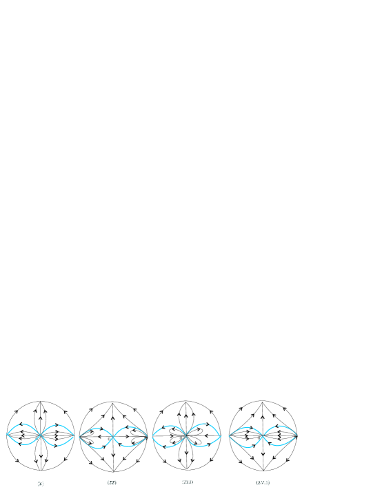
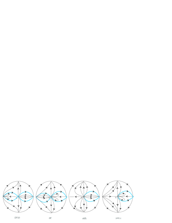
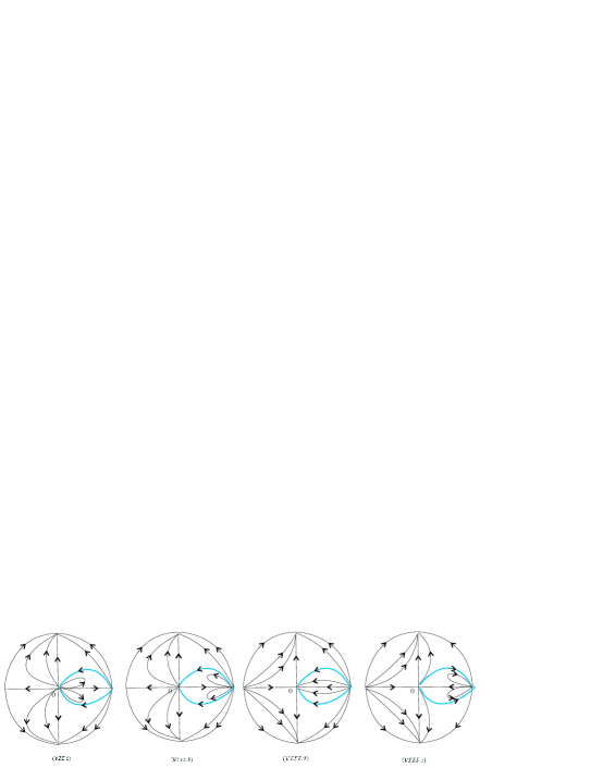
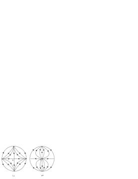
Figure 1. Global phase portraits of system $X_{111}$ as $a_{14}<1$.

In the case $a_{14}>1$, equilibrium $I_{1}$ is a saddle and we obtain the $24$ global phase portraits for the system $X_{111}$ by a similar research as the case $a_{14}<1$.

Tables 1 and 2 show the parameter conditions under which system $X_{111}$ has the phase portraits, where we have used the relation between the parameters of $X_{111}$ and $\mathcal{H}_{3}$, i.e. $c_{12}=a_{14}/(2b_{05})$, $c_{21}=a_{22}/(2b_{05})$, $c_{30}=a_{30}/(2b_{05})$, $d_{12}=b_{13}/b_{05}$, $d_{21}=b_{21}/b_{05}$. Note that each upper half part of the figure of system $\mathcal{H}_{3}$ is equivalent to some half part of the one in Figure 5.1 (1)–(14) of Cima and Llibre [8], which is also pointed out in Table 1 and Table 2.

Figure	parameter conditions	Figure 5.1 of [8]
Figure (I)	$\widehat{P}_{3}(u_{\pm})>0$, $\widehat{G}^{\prime}_{3}(u_{+})\widehat{G}^{\prime}_{3}(u_{-})>0$, $\widehat{P}_{3}(0)>0$	Figure (4)
Figure (I)	or $u_{1}=u_{11}$, $\widehat{P}_{3}(u_{1})>0$, $\widehat{G}^{\prime}_{3}(u_{1})\neq 0$, $\widehat{P}_{3}(0)>0$,
	or $u_{1}=u_{12}$, $\widehat{P}_{3}(u_{1})>0$, $\widehat{G}^{\prime}_{3}(u_{1})\neq 0$, $\widehat{P}_{3}(0)>0$,	Figure (8)
	or $u_{1}=u_{13}$, $\widehat{P}_{3}(u_{1})>0$, $\widehat{G}^{\prime\prime}_{3}(u_{1})\neq 0$, $\widehat{P}_{3}(0)>0$
Figure (I)	Condition ($\mathcal{C}_{31}$) or ($\mathcal{C}_{32}$), $\widehat{G}^{\prime}_{3}(0)\neq 0$, $\widehat{P}_{3}(0)>0$,	Figure (11)
	or Condition ($\mathcal{C}_{33}$), $\widehat{G}^{\prime\prime\prime}_{3}(0)\neq 0$, $\widehat{P}_{3}(0)>0$
Figure (I)	Condition ($\mathcal{C}_{33}$), $\widehat{G}^{\prime\prime}_{3}(0)\neq 0$, $\widehat{P}_{3}(0)>0$	Figure (13)
Figure (II)	$\widehat{P}_{3}(u_{\pm})<0$, $\widehat{G}^{\prime}_{3}(u_{\pm})>0$, $\widehat{P}_{3}(0)>0$	Figure (1)
Figure (III.1)	$\widehat{P}_{3}(u_{\pm})>0$, $\widehat{G}^{\prime}_{3}(u_{\pm})>0$, $\widehat{P}_{3}(0)<0$	Figure (5)
Figure (III.2)	$\widehat{P}_{3}(u_{+})\widehat{P}_{3}(u_{-})<0$, $\widehat{G}^{\prime}_{3}(u_{\pm})<0$, $\widehat{P}_{3}(0)>0$	Figure (5)
Figure (III.2)	or $u_{1}=u_{11}$, $\widehat{P}_{3}(u_{1})<0$, $\widehat{G}^{\prime}_{3}(u_{1})<0$, $\widehat{P}_{3}(0)>0$,
	or $u_{1}=u_{12}$, $\widehat{P}_{3}(u_{1})<0$, $\widehat{G}^{\prime}_{3}(u_{1})<0$, $\widehat{P}_{3}(0)>0$,	Figure (9)
Figure (III.3)	$\widehat{P}_{3}(u_{\pm})<0$, $\widehat{G}^{\prime}_{3}(u_{\pm})<0$, $\widehat{P}_{3}(0)<0$	Figure (5)
Figure (IV.1)	$\widehat{P}_{3}(u_{\pm})>0$, $\widehat{G}^{\prime}_{3}(u_{\pm})<0$, $\widehat{P}_{3}(0)<0$	Figure (2)
Figure (IV.2)	$\widehat{P}_{3}(u_{+})\widehat{P}_{3}(u_{-})<0$, $\widehat{G}^{\prime}_{3}(u_{\pm})>0$, $\widehat{P}_{3}(0)>0$	Figure (2)
Figure (IV.2)	or $u=u_{11}$, $\widehat{P}_{3}(u_{1})<0$, $\widehat{G}^{\prime}_{3}(u_{1})>0$, $\widehat{P}_{3}(0)>0$	Figure (6)
Figure (IV.3)	$\widehat{P}_{3}(u_{\pm})<0$, $\widehat{G}^{\prime}_{3}(u_{\pm})>0$, $\widehat{P}_{3}(0)<0$	Figure (2)
Figure (V.1)	$\widehat{P}_{3}(u_{+})\widehat{P}_{3}(u_{-})<0$, $\widehat{G}^{\prime}_{3}(u_{\pm})>0$, $\widehat{P}_{3}(0)<0$	Figure (3)
Figure (V.2)	$\widehat{P}_{3}(u_{+})\widehat{P}_{3}(u_{-})<0$, $\widehat{G}^{\prime}_{3}(u_{\pm})<0$, $\widehat{P}_{3}(0)<0$	Figure (3)
Figure (VI.1)	$u_{1}=u_{11}$, $\widehat{P}_{3}(u_{1})>0$, $\widehat{G}^{\prime}_{3}(u_{1})>0$, $\widehat{P}_{3}(0)<0$,	Figure (7)
Figure (VI.2)	$u_{1}=u_{12}$, $\widehat{P}_{3}(u_{1})<0$, $\widehat{G}^{\prime}_{3}(u_{1})<0$, $\widehat{P}_{3}(0)<0$	Figure (7)
Figure (VI.3)	$u_{1}=u_{13}$, $\widehat{P}_{3}(u_{1})<0$, $\widehat{G}^{\prime\prime}_{3}(u_{1})>0$, $\widehat{P}_{3}(0)>0$	Figure (7)
Figure (VI.4)	$u_{1}=u_{13}$, $\widehat{P}_{3}(u_{1})<0$, $\widehat{G}^{\prime\prime}_{3}(u_{1})<0$, $\widehat{P}_{3}(0)>0$	Figure (7)
Figure (VI.5)	$u_{1}=u_{11}$, $\widehat{P}_{3}(u_{1})>0$, $\widehat{G}^{\prime}_{3}(u_{1})<0$, $\widehat{P}_{3}(0)<0$,	Figure (7)
Figure (VI.6)	$u_{1}=u_{12}$, $\widehat{P}_{3}(u_{1})<0$, $\widehat{G}^{\prime}_{3}(u_{1})>0$, $\widehat{P}_{3}(0)<0$	Figure (7)
Figure (VII.1)	$u_{1}=u_{12}$, $\widehat{P}_{3}(u_{1})>0$, $\widehat{G}^{\prime}_{3}(u_{1})<0$, $\widehat{P}_{3}(0)<0$,	Figure (6)
	or $u_{1}=u_{13}$, $\widehat{P}_{3}(u_{1})>0$, $\widehat{G}^{\prime\prime}_{3}(u_{1})>0$, $\widehat{P}_{3}(0)<0$
Figure (VII.2)	$u_{1}=u_{12}$, $\widehat{P}_{3}(u_{1})<0$, $\widehat{G}^{\prime}_{3}(u_{1})>0$, $\widehat{P}_{3}(0)>0$	Figure (6)
Figure (VII.3)	$u_{1}=u_{11}$, $\widehat{P}_{3}(u_{1})<0$, $\widehat{G}^{\prime}_{3}(u_{1})>0$, $\widehat{P}_{3}(0)<0$,	Figure (6)
	or $u_{1}=u_{13}$, $\widehat{P}_{3}(u_{1})<0$, $\widehat{G}^{\prime\prime}_{3}(u_{1})>0$, $\widehat{P}_{3}(0)<0$
Figure (VIII.1)	$u_{1}=u_{12}$, $\widehat{P}_{3}(u_{1})>0$, $\widehat{G}^{\prime}_{3}(u_{1})>0$, $\widehat{P}_{3}(0)<0$,	Figure (9)
	or $u_{1}=u_{13}$, $\widehat{P}_{3}(u_{1})>0$, $\widehat{G}^{\prime\prime}_{3}(u_{1})<0$, $\widehat{P}_{3}(0)<0$
Figure (VIII.2)	$u_{1}=u_{11}$, $\widehat{P}_{3}(u_{1})<0$, $\widehat{G}^{\prime}_{3}(u_{1})<0$, $\widehat{P}_{3}(0)<0$,	Figure (9)
	or $u_{1}=u_{13}$, $\widehat{P}_{3}(u_{1})<0$, $\widehat{G}^{\prime\prime}_{3}(u_{1})<0$, $\widehat{P}_{3}(0)<0$
Figure (IX)	Condition ($\mathcal{C}_{31}$), $\widehat{G}^{\prime}_{3}(0)>0$, $\widehat{P}_{3}(0)<0$,
	or Condition ($\mathcal{C}_{32}$), $\widehat{G}^{\prime}_{3}(0)>0$, $\widehat{P}_{3}(0)<0$,	Figure (10)
	or Condition ($\mathcal{C}_{33}$), $\widehat{G}^{\prime\prime\prime}_{3}(0)>0$, $\widehat{P}_{3}(0)<0$
Figure (X)	Condition ($\mathcal{C}_{31}$) or ($\mathcal{C}_{32}$), $\widehat{G}^{\prime}_{3}(0)<0$, $\widehat{P}_{3}(0)<0$,	Figure (12)
	or Condition ($\mathcal{C}_{33}$), $\widehat{G}^{\prime\prime\prime}_{3}(0)<0$, $\widehat{P}_{3}(0)<0$
Figure (XI)	Condition ($\mathcal{C}_{33}$), $\widehat{G}^{\prime\prime}_{3}(0)\neq 0$, $\widehat{P}_{3}(0)<0$	Figure (14)

Table 1. Parameter conditions of figures (I)-(XI) as $a_{14}>1$.

Figure	parameter conditions	Figure 5.1 of [8]
Figure ($\mathcal{I}$)	$\widehat{P}_{3}(u_{\pm})>0$, $\widehat{G}^{\prime}_{3}(u_{\pm})>0$, $\widehat{P}_{3}(0)>0$	Figure (4)
Figure ($\mathcal{II}$)	$\widehat{P}_{3}(u_{\pm})<0$, $\widehat{G}^{\prime}_{3}(u_{\pm})>0$, $\widehat{P}_{3}(0)>0$	Figure (1)
Figure ($\mathcal{III}$)	$\widehat{P}_{3}(u_{\pm})>0$, $\widehat{G}^{\prime}_{3}(u_{\pm})>0$, $\widehat{P}_{3}(0)<0$	Figure (5)
Figure ($\mathcal{IV}$.1)	$\widehat{P}_{3}(u_{\pm})<0$, $\widehat{G}^{\prime}_{3}(u_{\pm})>0$, $\widehat{P}_{3}(0)<0$	Figure (2)
Figure ($\mathcal{IV}$.2)	$\widehat{P}_{3}(u_{+})\widehat{P}_{3}(u_{-})<0$, $\widehat{G}^{\prime}_{3}(u_{\pm})>0$, $\widehat{P}_{3}(0)>0$	Figure (2)
Figure ($\mathcal{V}$)	$\widehat{P}_{3}(u_{+})\widehat{P}_{3}(u_{-})<0$, $\widehat{G}^{\prime}_{3}(u_{\pm})>0$, $\widehat{P}_{3}(0)<0$	Figure (3)
Figure ($\mathcal{VI}$)	$u_{1}=u_{11}$, $\widehat{P}_{3}(u_{1})>0$, $\widehat{G}^{\prime}_{3}(u_{1})>0$, $\widehat{P}_{3}(0)>0$,	Figure (8)
	or $u_{1}=u_{13}$, $\widehat{P}_{3}(u_{1})>0$, $\widehat{G}^{\prime\prime}_{3}(u_{1})>0$, $\widehat{P}_{3}(0)>0$
Figure ($\mathcal{VII}$.1)	$u_{1}=u_{11}$, $\widehat{P}_{3}(u_{1})>0$, $\widehat{G}^{\prime}_{3}(u_{1})>0$, $\widehat{P}_{3}(0)<0$,	Figure (7)
Figure ($\mathcal{VII}$.2)	$u_{1}=u_{13}$, $\widehat{P}_{3}(u_{1})<0$, $\widehat{G}^{\prime\prime}_{3}(u_{1})>0$, $\widehat{P}_{3}(0)>0$	Figure (7)
Figure ($\mathcal{VIII}$.1)	$u_{1}=u_{11}$, $\widehat{P}_{3}(u_{1})<0$, $\widehat{G}^{\prime}_{3}(u_{1})>0$, $\widehat{P}_{3}(0)>0$	Figure (6)
Figure ($\mathcal{VIII}$.2)	$u_{1}=u_{11}$, $\widehat{P}_{3}(u_{1})<0$, $\widehat{G}^{\prime}_{3}(u_{1})>0$, $\widehat{P}_{3}(0)<0$,	Figure (6)
	or $u_{1}=u_{13}$, $\widehat{P}_{3}(u_{1})<0$, $\widehat{G}^{\prime\prime}_{3}(u_{1})>0$, $\widehat{P}_{3}(0)<0$
Figure ($\mathcal{VIII}$.3)	$u_{1}=u_{13}$, $\widehat{P}_{3}(u_{1})>0$, $\widehat{G}^{\prime\prime}_{3}(u_{1})>0$, $\widehat{P}_{3}(0)<0$	Figure (6)
Figure ($\mathcal{IX}$)	Condition ($\mathcal{C}_{33}$), $\widehat{G}^{\prime\prime\prime}_{3}(0)>0$, $\widehat{P}_{3}(0)<0$	Figure (10)
	or Condition ($\mathcal{C}_{31}$), $\widehat{G}^{\prime}_{3}(0)>0$, $\widehat{P}_{3}(0)<0$
Figure ($\mathcal{X}$)	Condition ($\mathcal{C}_{31}$), $\widehat{G}^{\prime}_{3}(0)>0$, $\widehat{P}_{3}(0)>0$,	Figure (11)
	or Condition ($\mathcal{C}_{33}$), $\widehat{G}^{\prime\prime\prime}_{3}(0)>0$, $\widehat{P}_{3}(0)>0$

Table 2. Parameter conditions of figures ($\mathcal{I}$)-($\mathcal{X}$) as $a_{14}<1$.

At last, we consider the case $a_{14}=1$, which implies that $c_{12}=1/2$ and the infinity fulfils singularities. Besides, by a time rescaling $d\tau_{2}=zd\tau_{1}$, system (32) becomes

(38) $$\begin{cases}\dot{v}=v((a_{22}-b_{13})v+(a_{30}-b_{21})v^{2}z),\\ \dot{z}=-(1+b_{13}vz+b_{21}v^{2}z^{2}).\end{cases}$$

Clearly, system (38) has no singularities on the axis $z=0$. Note that the global structures of system (38) and system (32) are equivalent outside $z=0$. Hence, except the $y$–axis no orbits connect the singularities at infinity of system $X_{111}$ other than $I_{0}$. Similar to the case $a_{14}<1$, we also have exactly the 14 subcases given in Table 2, and consequently we will obtain 14 different topological phase portraits, which are different from those in the case $a_{14}>1$ only now the infinity fulfils singularities instead of the invariant line at infinity.

Summarizing the above analysis, we get that system $X_{111}$ has totally 52 topological phase portraits without taking into account direction of the time. We complete the proof of the theorem. ∎

Finally we study topological structures of the homogeneous system $\mathcal{H}_{2}$, which corresponds to the quasi–homogeneous systems $X_{011}$, $X_{113}$ and $X_{131}$.

Theorem 12.

The global phase portraits of the quintic quasi–homogeneous systems $X_{011}$, $X_{113}$ and $X_{131}$ are topologically equivalent to one of the phase portraits in Figs. 2 and 3 without taking into account the direction of the time.

Proof.

Since the homogeneous systems associated to $X_{113}$ and $X_{131}$ are sub–systems of the homogeneous systems associated to $X_{011}$ with $a_{05}=b_{20}=0$, we only need to study system $X_{011}$ for arbitrary $a_{05}$ and $b_{20}$.

Similar to the discussion of the cubic homogeneous system $\mathcal{H}_{3}$ in Theorem 11, we set

$$\mathcal{H}_{2}:=(P_{2}(x,y),Q_{2}(x,y))\quad\mbox{and}\quad G_{2}(x,y)=xQ_{2}(x,y)-yP_{2}(x,y).$$

Through the change of variables between the quasi-homogeneous differential systems and their associated homogeneous ones we get that the invariant line $y=u_{0}x$ of system $\mathcal{H}_{2}$ as $u_{0}\neq 0$ corresponds to an invariant curve of system $X_{011}$, which is tangent to the $y$–axis at the origin, and connects the origin and the singularity at infinity located at the end of $x$-axis. Moreover, this invariant curve of system $X_{011}$ is usually a separatrix of hyperbolic sectors, parabolic sectors or elliptic sectors, which is drawn in thick blue curves in Fig. 2. Note that $G_{2}(x,y)$ is of degree three. It follows that $X_{011}$ has at least one characteristic direction at the origin. From [26, Chapter 10], we can move the characteristic direction to the $x$–axis and system $\mathcal{H}_{2}$ can be written by a linear transformation as

(39) $$\begin{cases}\dot{x}_{1}=\alpha_{11}x_{1}^{2}+\alpha_{12}x_{1}y_{1}+\alpha_{22}y_{1}^{2},\\ \dot{y}_{1}=\beta_{12}x_{1}y_{1}+\beta_{22}y_{1}^{2}.\end{cases}$$

Since system $\mathcal{H}_{2}$ has no a common factor, and so is system (39). It forces that $\alpha_{11}\neq 0$. Using the inverse of change (22), we transform system (39) into

(40) $$\begin{cases}\dot{x}=\alpha_{11}x^{2}+\alpha_{12}xy^{2}+\alpha_{22}y^{4},\\ \dot{y}=(\beta_{12}xy+\beta_{22}y^{3})/2.\end{cases}$$

Taking the Poincaré transformations $x=v/z,\,y=1/z$ together with the time rescaling $dt_{1}=z^{3}dt$, system (40) around the equator of the Poincaré sphere can be written in

(41) $$\begin{cases}\dot{v}=\alpha_{22}+(\alpha_{12}-\frac{\beta_{22}}{2})vz+(\alpha_{11}-\frac{\beta_{12}}{2})v^{2}z^{2},\\ \dot{z}=-z^{2}(\frac{\beta_{22}}{2}+\frac{\beta_{12}}{2}vz).\end{cases}$$

Therefore, system (40) has a unique singularity at the infinity when $\alpha_{22}\neq 0$, which is $\tilde{I}_{0}$ located at the end of the $x$–axis. When $\alpha_{22}=0$, the infinity of system (40) is fulled up with singularities. Moving away the common factor $z$ of system (41), the new system has a unique singularity on $z=0$, i.e. $\widetilde{I}_{1}$, which is at the end of the $y$–axis. For this new system we can check that $\tilde{I}_{1}$ is either a saddle if $(2\alpha_{12}-\beta_{22})\beta_{22}>0$, or a node if $(2\alpha_{12}-\beta_{22})\beta_{22}<0$. Moreover, under the condition $\alpha_{22}=0$ we can show that system (40) has always the singularity $\tilde{I}_{0}$ at the end of the $x$–axis, which is degenerate. When $\beta_{22}=0$ and $\alpha_{22}=0$, system (39) has a common factor, which is out of our consideration. When $2\alpha_{12}-\beta_{22}=0$, $\beta_{22}\neq 0$ and $\alpha_{22}=0$, moving away the common factor $z^{2}$ of system (41), the new system has no singularities on $z=0$.

Having the above preparation, we now study the global phase portraits of system $X_{011}$ according to the number of the zeros of $\widehat{G}_{2}(u):=G_{2}(1,u)$, which can have either one, or two, or three real roots. The next results can be obtained by using [26, Theorem 10.5], the details are omitted.

Case $(i)$. $\widehat{G}_{2}(u)$ has three different real zeros. Then we obtain the $3$ global phase portraits given in Fig. 2 for the system $X_{011}$.

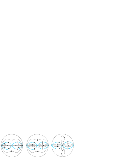
Figure 2. Phase portraits of $X_{011}$ in case $(i)$.

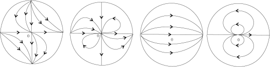
Figure 3. Phase portraits of $X_{011}$ in case $(ii)$ and case $(iii)$.

Case $(ii)$. $\widehat{G}_{2}(u)$ has two different real zeros. Then we get $2$ global phase portraits, which are given in the first two figures of Fig. 3 for system $X_{011}$.

Case $(iii)$. $\widehat{G}_{2}(u)$ has only one real zero. Then we obtain $2$ global phase portraits, which are given in the last two figures of Fig. 3 for system $X_{011}$.

We complete the proof of the theorem. ∎

We remark that the quintic quasi–homogeneous system other than $X_{111}$, $X_{011}$, $X_{113}$ and $X_{131}$ either has a nondegenerate linear part, or can be reduced to a linear system, or to a constant system by using Lemma 5 and Theorem 1. Hence, their global structures are not difficult to be obtained. The details are omitted here.

By Theorem 1 and 6 we can prove easily the results of [24, Theorem 1.2]. In fact, only system $X_{021}$ in all quintic quasi–homogeneous but non–homogeneous systems can have a center at the origin when $a_{12}=-3b_{03}$ and $a_{12}b_{03}-a_{05}b_{10}>0$. And only in this case, the linear system $\widetilde{X}_{021}$ translated from $X_{021}$ and given in the proof of Theorem 6 has a pair of conjugate pure imaginary eigenvalues.

References

- [1] Algaba A., Fuentes N., García C., Center of quasihomogeneous polynomial planar systems, Nonlinear Anal. Real World Appl. 13 (2012), 419–431.
- [2] Algaba A., Gamero E., García C., The integrability problem for a class of planar systems, Nonlinearity 22 (2009), 396–420.
- [3] Algaba A., García C., Reyes M., Rational integrability of two dimensional quasi–homogeneous polynomial differential systems, Nonlinear Anal. 73 (2010), 1318–1327.
- [4] Aziz W., Llibre J., Pantazi C., Centers of quasi–homogeneous polynomial differential equations of degree three, Adv. Math. 254 (2014), 233–250.
- [5] Briot Ch., Bouquet J. C., Recherches sur les proprits des fonctions dfinies par des quations diffrentielles, J. cole Imp. Polyt. 21(1856), 133–197.
- [6] Cairó L., Llibre J., Polynomial first integrals for weighthomogeneous planar polynomial differential systems of weight degree 3, J. Math. Anal. Appl. 331 (2007), 1284–1298.
- [7] Chow S. N., Hale J. K., Methods of Bifurcation Theory, Springer–Verlag, Berlin, 1982.
- [8] Cima A., Llibre J., Algebraic and topological classification of the homogeneous cubic systems in the plane, J. Math. Anal. Appl. 147 (1990), 420–448.
- [9] Date T., Classification and analysis of two-dimensional homogeneous quadratic differential equations systems, J. Diff. Eqns. 32 (1979), 311–334.
- [10] Dumortier F., Llibre J., Artés J. C., Qualititive theory of planar differential systems, Springer–Verlag, Berlin, 2006.
- [11] García I., On the integrability of quasihomogeneous and related planar vector fields, Intern. J. Bifur. Chaos 13 (2003), 995–1002.
- [12] García B., Llibre J., Pérez del Río J. S., Planar quasihomogeneous polynomial differential systems and their integrability, J. Diff. Eqns. 255 (2013), 3185–3204.
- [13] Gavrilov L., Giné J., Grau M., On the cyclicity of weight-homogeneous centers, J. Diff. Eqns. 246 (2009), 3126–3135.
- [14] Giné J., Grau M., Llibre J., Polynomial and rational first integrals for planar quasi-homogeneous polynomial differential systems, Discrete Contin. Dyn. Syst. 33 (2013), 4531–4547.
- [15] Goriely A., Integrability, partial integrability, and nonintegrability for systems of ordinary differential equations, J. Math. Phys. 37 (1996), 1871–1893.
- [16] Hu Y., On the integrability of quasihomogeneous systems and quasidegenerate infinity systems, Adv. Difference Eqns. (2007), Art ID 98427, 10 pp.
- [17] Li W., Llibre J., Yang J., Zhang Z., Limit cycles bifurcating from the period annulus of quasi–homegeneous centers, J. Dyn. Diff. Eqns. 21 (2009), 133–152.
- [18] Liang H., Huang J., Zhao Y., Classification of global phase portraits of planar quartic quasi–homogeneous polynomial differential systems, Nonlinear Dynam.78 (2014), 1659–1681.
- [19] Llibre J., Pérez del Río J. S., Rodríguez J. A., Structural stability of planar homogeneous polynomial vector fields. Applications to critical points and to infinity, J. Diff. Eqns. 125 (1996), 490–520.
- [20] Llibre J., Zhang X., Polynomial first integrals for quasihomogeneous polynomial differential systems, Nonlinearity 15 (2002), 1269–1280.
- [21] Newton T. A., Two dimensional homogeneous quadratic differential systems, SIAM Review 20 (1978), 120–138.
- [22] Sansone G., Conti R., Non-Linear Differential Equations, Pergamon Press, New York, 1964.
- [23] Sibirskii K. S., Vulpe N. I., Geometric classification of quadratic differential systems, Differential Equations 13 (1977), 548–556.
- [24] Tang Y., Wang L., Zhang X., Center of planar quintic quasi– homogeneous polynomial differential systems, Discrete Contin. Dyn. Syst. 35 (2015), 2177–2191.
- [25] Vdovina E. V., Classification of singular points of the equation by Forster’s method (Russian), Diff. Uravn. 20 (1984), 1809–1813.
- [26] Ye Y. Q., Theory of Limit Cycles, Trans. Math. Monographs 66, Amer. Math. Soc. Providence, RI, 1984.
- [27] Ye Y. Q., Qualitative Theory of Polynomial Differential Systems, Shanghai Science Technology Pub., Shanghai, 1995.
- [28] Yoshida H., Necessary conditions for existence of algebraic first integrals I and II, Celestial Mech. 31 (1983), 363–379, 381–399.
- [29] Zhang Z. F., Ding T. R., Huang W. Z., Dong Z. X., Qualitative Theory of Differential Equations, Transl. Math. Monographs 101, Amer. Math. Soc., Providence, 1992.