Tomlinson model improved with no ad-hoc dissipation

Abstract

The origin of friction force is a very old problem in physics, which goes back to Leonardo da Vinci or even older times. Extremely important from a practical point of view, but with no satisfactory explanation yet. Many models have been used to study dry sliding friction. The model introduced in the present work consists in one atom that slide over a surface represented by a periodic arrangement of atoms, each confined by an independent harmonic potential. The novelty of our contribution resides in that we do not include an ad hoc dissipation term as all previous works have done. Despite the apparent simplicity of the model it can not be solved analytically, so the study is performed solving the Newton’s equations numerically. The results obtained so far with the present model are in accordance with the Tomlinson model, often used to represent the atomic force microscope. The atomic-scale analysis of the interaction between sliding surfaces is necessary to understand the non-conservative lateral forces and the mechanism of energy dissipation which can be thought as effective emerging friction.

I Introduction

Friction is one of the most important problems and a key phenomenon in physics and engineering, whose fundamental origin has been studied for centuries and still remains controversial  Krim2002 ; Persson2000 ; Makkonen2012 . From Leonardo da Vinci, Coulomb and Rynolds, sliding friction has been a topic of great interest studies intensively by many of the brightest scientists. In the last years, theoretical models for atomic friction, mostly based on the early work of Tomlinson  Tomlinson1929 , and Frenkel-Kontorova Kontorova ; Frenkel ; braun2004frenkel models, were proposed and characterized by being highly simplified and yet retaining enough complexity to exibit interesting features  Buldum1997 ; Goncalves2004 ; Goncalves2005 ; Tiwari2008 ; Fusco2005 ; Neide2010 . Such models have allowed to explain essential features of atomic-scale friction such as the occurrence of the ”stick-slip” phenomenon observed in the movement of the tip over a surface material in the friction force microscope (FFM)  Tomanek1991 ; Gyalog1996 . Friction is the result of the transformation of sliding motion into heat or different forms of energy, i.e., is the dissipated energy per unit length  Helman1994 ; Wang2015 , where the frictional work it is assumed to be dissipated through plastic deformation and material damage  Bowden1951 . In the Tomlinson model, the energy dissipation is attributed to the instability induced by the stick-slip motion and consequent atomic vibration. What is expected is to increase the control over the mechanisms of friction and thus reduce the loss of energy. In this contribution we aim to understand the fundamental mechanisms on these energy exchange between the tip and the surface without include any ad hoc dissipation term as previous works have done. We want to show that without the ad hoc term, the energy lost by the tip is absorbed by the substrate. Despite the apparent simplicity of the model it can not be solved analytically, so the study is performed solving the Newton’s equations numerically. demonstrate that the energy dissipation is almost all absorbed by the stiffness of the substrate

II Model

The proposed model in the present study aims to explore the effect of various parameters involved on the emergence of frictional force and how the energy generated during the process is dispersed when there is no ad hoc dissipation. In this sense, our model in Fig. 1 was never presented in previous works. The tip is represented by a particle of mass $M$, connected by a spring of constant $K$ to a driven support that moves at constant velocity $v_{c}$. The substrate is represented by a series of particle-spring systems of mass $m$ and constant $k$, independent between them , but interacting with the tip via a short range Gaussian type potential. To avoid edge effects we modeled the chain as being infinite.

Figure 1: Diagram of the model proposed in this work.

The system is described by the Hamiltonian

$$H=\frac{P^{2}}{2M}+\sum_{i=1}^{N}\frac{p^{2}}{2m}+\sum_{i=1}^{N}U(X,x_{i})+U(X)+\sum_{i=1}^{N}U(x_{i})$$ (1)

where $X,P$ and $x,p$ are the tip and substrate coordinates respectively; $U(X,x_{i})=U_{0}e^{-\frac{(X-x_{i})^{2}}{\sigma^{2}}}$ is the interaction between the tip and each of the particles of the substrate. We choose the value of $\sigma$ in such a way that the Gaussian potential of each particle does not overlap with that of its neighbors. So the tip can interact with each of them separately.
In this case, $\sigma=a_{x}/n$, where $a_{x}$ is the separation between the particles of the substrate and $n$ is a constant. $U(X)=\frac{K}{2}(X-x_{c})^{2}$ is the elastic interaction between the tip and the cantilever. The support position $x_{c}$ is $x_{c}=v_{c}t$. And $U(x_{i})=\frac{k}{2}(x_{i}-x^{0}_{i})^{2}$ is the elastic potential of each particle (independent between them).

This results in the following equation of motion:

$$\begin{aligned} \begin{multlined}M\ddot{X}=-K(X-v_{c}t)\\ +\frac{2U_{0}}{\sigma^{2}}\sum_{i=1}^{N}(X-x_{i})e^{-\frac{(X-x_{i})^{2}}{\sigma^{2}}}\\ \end{multlined}M\ddot{X}=-K(X-v_{c}t)\\ +\frac{2U_{0}}{\sigma^{2}}\sum_{i=1}^{N}(X-x_{i})e^{-\frac{(X-x_{i})^{2}}{\sigma^{2}}}\\ \end{aligned}$$ (2)

$$\begin{aligned} \begin{multlined}m\sum_{i=1}^{N}\ddot{x_{i}}=-k\sum_{i=1}^{N}(x_{i}-x_{0_{i}})\\ -\frac{2U_{0}}{\sigma^{2}}\sum_{i=1}^{N}(X-x_{i})e^{-\frac{(X-x_{i})^{2}}{\sigma^{2}}}\end{multlined}m\sum_{i=1}^{N}\ddot{x_{i}}=-k\sum_{i=1}^{N}(x_{i}-x_{0_{i}})\\ -\frac{2U_{0}}{\sigma^{2}}\sum_{i=1}^{N}(X-x_{i})e^{-\frac{(X-x_{i})^{2}}{\sigma^{2}}}\end{aligned}$$ (3)

Introducing the adimensional units $Q=\frac{X}{\sigma},q=\frac{x}{\sigma},\tau=\sqrt{\frac{K}{M}}t,\tilde{U_{0}}=\frac{2U_{0}}{k_{t}\sigma^{2}},\tilde{v_{c}}=\frac{v_{c}}{\sigma}\sqrt{\frac{M}{K}}$ , the equations  2 and  3 can be reduced to:

$$\ddot{Q}=-q+\tilde{v_{c}}\tau+\tilde{U_{0}}\sum_{i=1}^{N}(Q-q_{i})e^{-(q_{t}-q_{s_{i}})^{2}}$$ (4)

$$\begin{aligned} \begin{multlined}\sum_{i=1}^{N}\ddot{q}_{i}=\frac{\epsilon_{1}}{\epsilon_{2}}\sum_{i=1}^{N}(q_{i}-q_{0_{i}})\\ -\epsilon_{1}\tilde{U_{0}}\sum_{i=1}^{N}(Q-q_{i})e^{-(Q-q_{i})^{2}}\end{multlined}\sum_{i=1}^{N}\ddot{q}_{i}=\frac{\epsilon_{1}}{\epsilon_{2}}\sum_{i=1}^{N}(q_{i}-q_{0_{i}})\\ -\epsilon_{1}\tilde{U_{0}}\sum_{i=1}^{N}(Q-q_{i})e^{-(Q-q_{i})^{2}}\end{aligned}$$ (5)

where $\epsilon_{1}=M/m$ is the ratio of the mass of the tip and the substrate particles (assuming all have the same masses) and $\epsilon_{2}=K/k$ is the ratio of the stiffness of the tip and the substrate.

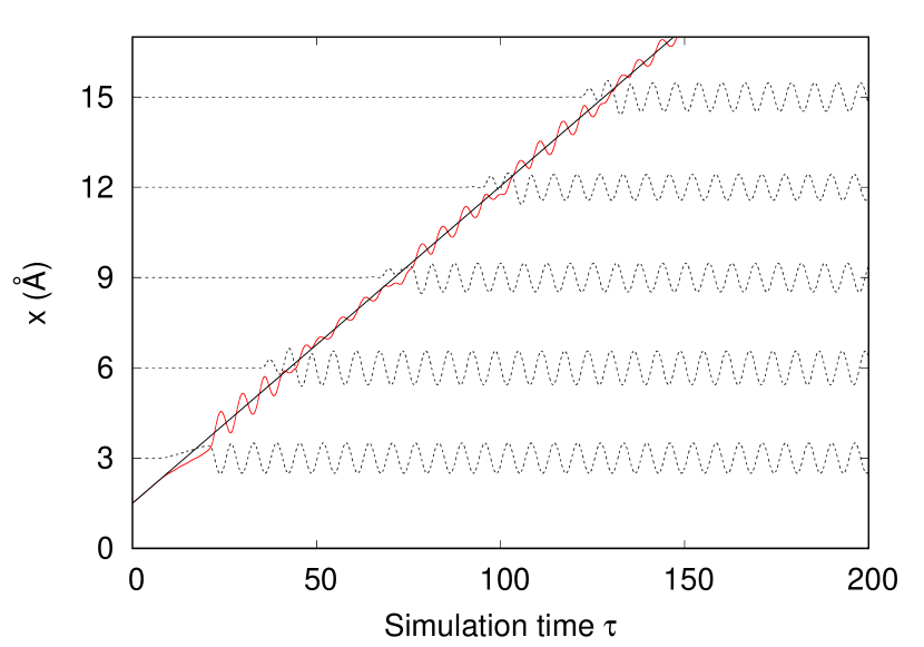
Figure 2: Position of the tip and the cantilever guide in straight line. The dashed lines represents the first five perturbed particles.

.

III Methods

The problem was solved numerically by using classical molecular-dynamics methods  Allen1987 ; Frenkel2002 using a set of realistic parameters Zworner1998 ; Fusco2005 ; Wang2015 , $M=m=10^{-10}$ $kg$, $K=k=10$ $N/m$, $a_{x}=3$ $\AA$, $U_{0}=0.085$ $eV$, $v_{c}=1$ $\mu m/seg$ which are typical of an AFM experiments  Bennewitz1999 ; Holscher1997 .
The most evident consequence of not having dissipation is that the particles that are perturbed by the tip do not return to their initial state, remaining oscillating infinitely, as it is presented on Fig. 2 for the first five particles in dashed lines.
For the frictional force calculation we compare three different methods.

It is known that $F$ is defined as the mean value of the lateral force  Holscher1997 ; Zworner1998 ; Fusco2005 ; Helman1994 . Since the problem is in one dimension, from here, we will refer to the lateral force as friction force $F$.

$$F=K(X-x)=K(X-v_{c}t)$$ (6)

The second way to obtain $F$ is through the energy accumulated by the substrate. The power is the instantaneous product of force times velocity and the time derivative of energy.

$$F\ v_{c}=\frac{dE}{dt}$$ (7)

From this relation, it is possible to obtain the frictional force as the slope of the total substrate energy by linear regression. Another method to calculate the friction force in these mechanical problem is calculating the average of the force between the tip and the substrate generated by the gaussian interaction force. These three methods are compared in Fig. 3 with their respective error bars.

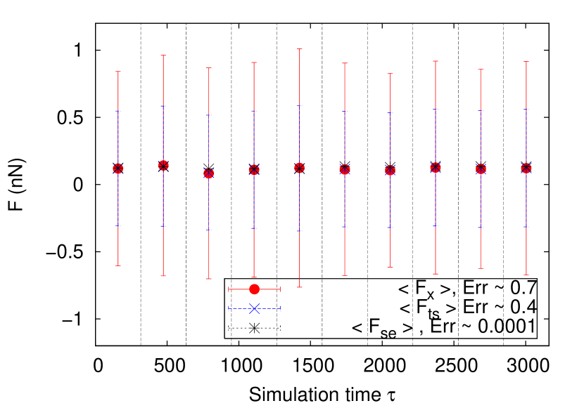
Figure 3: Comparison of the friction force values for the three methods of calculation, and their respective error bars

.

The total simulation time $\tau$ was divided into ten equal regions. For each of these intervals, the mean of the force was calculated in order to compare their values. $<F_{x}>$ represents the value obtained from eq.  3, $<F_{ts}>$ from the gaussian potential between the tip and the substrate; and $<F_{se}>$ is the slope of the accumulated energy of the substrate.

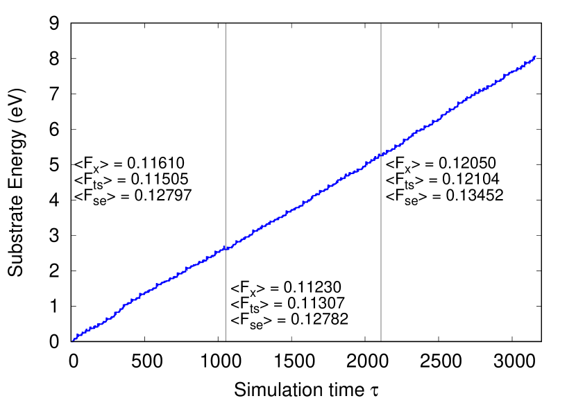
Figure 4: Comparison of the lateral force values for the three methods in diferents times

.

In Fig. 4 it is shown the accumulation of energy by the substrate and the values of the frictional force obtained by the three methods. In this case, $\tau$ was divided into three regions.

The comparison of the three methods shows that the smallest error in the measurements corresponds to the force obtained through the energy accumulated by the substrate. For this reason, we have chosen it to perform the rest of the simulations where all the parameters of the model will be analyzed.

III.1 Time step comparation

Molecular dynamics simulation is a technique by which, step by step, the equations of motion that describe the Newton’s classical mechanics are solved  Allen1987 ; Rapaport1995 ; Frenkel2002 . In the process of integrating the equations, the common important parameter is the time step $\Delta t$. If a big time step is used, the motion of molecule becomes unstable due to the very big error occurring in the integration.

If a big time step is chosen, the MD simulation becomes unstable due to the very big error in the integration process, not showin behaviours existing in the mechanical problem. If the time step is very small, the simulation will not be efficient due to a very long calculation time.

Earlier works  Grubmuller1998 ; Choe2000 have been demonstrated that stable dynamics will be executed only with the use of the smaller time step compared to the period of the highest vibrational frequency. Determining the biggest time step for a stable dynamics, will maximize the efficiency of the molecular dynamics simulation.

For these reason and since every mechanical problem is differnet from each other we decide to solve the equations for several time steps in order to choose the indicated such that not take long simulation time but at the same time we can extract reliable results referring to the lateral force.

Fig.  5 shows the energy of the substrate (kinetic energy plus elastic potential energy) for differents ${\Delta}t$ :from 0.001 to 10 [ns]. As we are interested in getting the value of $F_{x}$ from the slope of the curve, it can be observed that the choose of higher or lower time steps doesnt affect significantly the final result. The difference can be visualized in graphs such as position,velocity or $F_{x}$ itself, where for small values of ${\Delta}t$, oscillations of the tip are missing. In conclusion, for the numerical simulations we choose ${\Delta}t=0.1ns$.

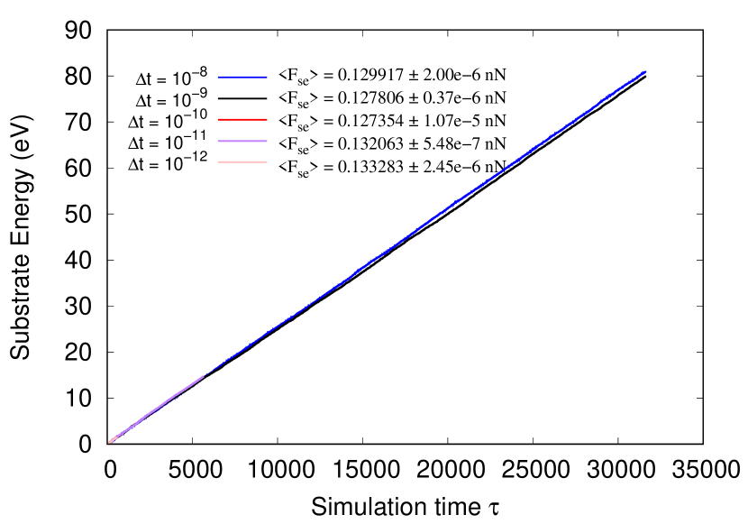
Figure 5: Substrate energy for different different time-steps

.

IV Results

Once the method and the time step have been chosen, we calculate $F$ varying each of the parameters of the model. The variation of $F$ with the velocity of the driven support it is shown in Fig. 6. For small velocities $v_{c}<1$ $\mu m$, $F$ remains constant and for higher values, it drops to zero. This is expected since the model does not have a velocity-dependent damping term. The total energy of the substrate decreases as the support velocity increases because the tip does not interact enough time with the substrate particles. As a consequence, the amplitude of oscillation around the equilibrium position is not significant.

Figure 6: Lateral Friction Force in function of the velocity of the cantilever. The other parameters were $M=m=10^{-10}$ $kg$, $K=k=10$ $N/m$, $a_{x}=3$ $\AA$, $U_{0}=0.085$ $eV$

.

When the variable parameter is the elasticity $k$ of the substrate particles (Fig. 7), we can identify a behavior of the shape $F=1/k^{n}$ in three differents regions. For the first interval, $k<1$ $N/m$, the adjustment parameter is $n=1$. This means that as $k$ increases, $F$ decreases. The softer the material, the higher the energy lost. When 1 $N/m<k<130$ $N/m$ there is an unpredictable region with maximums and minimums. Although there is an oscillation in the values of the friction, we assume that the average value remains constant. For that reason, the parameter $n\approx 0.26$. The third region, shows a more expected result. Due to the hardness of the substrate, the particles do not deviate from their equilibrium position, so the elastic potential is almost null as well as the kinetic energy. In these region, the parameter $n=4$.

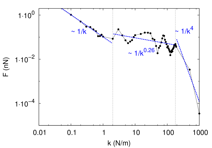
Figure 7: Lateral Friction Force with substrate spring stiffness. The other parameters were $M=m=10^{-10}$ $kg$, $K=10$ $N/m$, $a_{x}=3$ $\AA$, $U_{0}=0.085$ $eV$, $v_{c}=1$ $\mu m/seg$

.

The variation of the friction with the amplitude of the potential $U_{0}$, reproduced in Fig. 8, follows the shape $F=mU_{0}$, where again $m$ varies for three different regions. In this case, since the data is better visualized and interpreted in linear scale, we did not see the need to represent the results in logarithmic scale. It can be observed that $F$ increase with the high of potential energy following the shape When $U_{0}$ is up to $0.5eV$, $m\approx 1.81$. The friction almost doubles its value for each increment in $U_{0}$. For the second region, the growth rate decreases to a quarter of the presented in the first interval, here $m\approx 0.46$. And for the third interval, the growth is already very small, taking into account that it represents the eighth part of the first region growth. This is because the tip remains in between two particles for more time (while the support advances), as the amplitude increases.

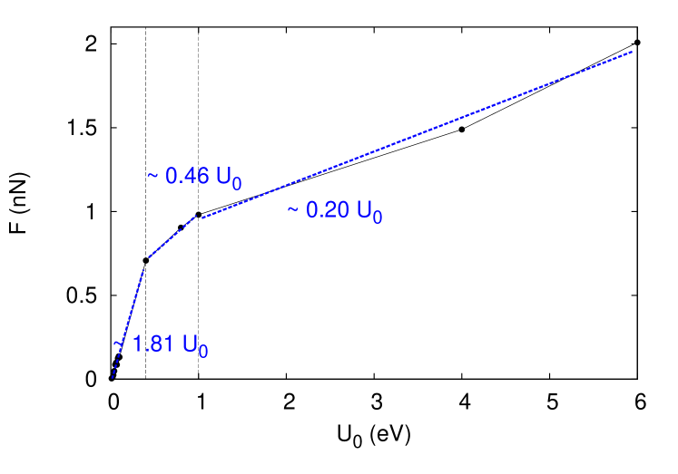
Figure 8: Lateral Friction Force in function of the potential high. The other parameters were: $M=m=10^{-10}$ $kg$, $K=k=10$ $N/m$, $a_{x}=3$ $\AA$, $v_{c}=1$ $\mu m/seg$

.

The last Figure correspond to the friction force behavior with the mass ratio between the particles of the substrate and the tip $m/M$ (Fig. 9). We can see that when $m<M$ the frictional force mantains its constant value, then begins to decrease until reaching a minimum, corresponding to $m=2M$. After this point increases again and for a small gap of values between $m=5M$ and $m=10M$ again $F$ shows independent on the masses ratio. Finally, fall to zero for very large substrate masses. When the nasses are too big, the potential energy of the substrate is very small since the mass of the tip does not manage to move them.

Figure 9: Lateral Friction Force in function of the masses ratio. The other parameters were: $K=k=10$ $N/m$, $a_{x}=3$ $\AA$, $U_{0}=0.085$ $eV$, $v_{c}=1$$\mu m/seg$

.

V Conclusion

In this paper we investigated a simple model to understand the fundamental mechanisms on the energy exchange in dry friction without include any ad hoc dissipation term as previous works have done. We compare three different methods to calculate de friction force in order to obtain the most accurate value. The work was performed solving the Newton’s equations numerically, for differents $\Delta t$ with the aim of gain computational time. We study the variations of $F$ variyng all the parameters involved in the description of the model We could show that the energy lost by the tip is absorbed by the substrate. Our gol in the future is to study the same model by placing particles of different masses in the substrate and $T\neq 0$ to obserbe how evolves

VI Acknowledgments

This work was supported by the Centro Latinoamericano de Física (CLAF) and the Conselho Nacional de Desenvolvimento Científico e Tecnológico (CNPq,Brazil).

References

- (1) J. Krim, “Surface science and the atomic-scale origins of friction: what once was old is new again,” Surface Science, vol. 500, no. 1–3, pp. 741 – 758, 2002.
- (2) B. N. J. Persson, Sliding Friction. Springer Berlin Heidelberg, 2000.
- (3) L. Makkonen, “A thermodynamic model of sliding friction,” AIP Advances, vol. 2, no. 1, p. 012179, 2012.
- (4) G. Tomlinson, “CVI. A molecular theory of friction,” The London Edinburgh, and Dublin Philosophical Magazine and Journal of Science, vol. 7, pp. 905–939, jun 1929.
- (5) Frenkel, J and Kontorova, T,“On the theory of plastic deformation and twinning,” Izv. Akad. Nauk, Ser. Fiz., vol. 1,pp. 137-149, 1939
- (6) Kontorova, T and Frenkel, J, “On the theory of plastic deformation and twinning. II.”, Zh. Eksp. Teor. Fiz., vol. 8,pp. 1340-1348,1938
- (7) Braun, O.M. and Kivshar, Y.S.,“The Frenkel-Kontorova Model: Concepts, Methods, and Applications,” Physics and Astronomy Online Library,Springer, 2004
- (8) Bennewitz, R. and Gyalog, T. and Guggisberg, M. and Bammerlin, M. and Meyer, E. and Güntherodt, H.-J, “Atomic-scale stick-slip processes on Cu(111),”Phys. Rev. B, vol. 60,pp. R11301–R11304,oct 1999.
- (9) A. Buldum and S. Ciraci, “Atomic-scale study of dry sliding friction,” Phys. Rev. B, vol. 55, pp. 2606–2611, Jan 1997.
- (10) S. Gonçalves, V. M. Kenkre, and A. R. Bishop, “Nonlinear friction of a damped dimer sliding on a periodic substrate,” Phys. Rev. B, vol. 70, nov 2004.
- (11) S. Gonçalves, C. Fusco, A. R. Bishop, and V. M. Kenkre, “Bistability and hysteresis in the sliding friction of a dimer,” Phys. Rev. B, vol. 72, p. 195418, Nov 2005.
- (12) M. Tiwari, S. Gonçalves, and V. M. Kenkre, “Generalization of a nonlinear friction relation for a dimer sliding on a periodic substrate,” The European Physical Journal B, vol. 62, pp. 459–464, apr 2008.
- (13) C. Fusco and A. Fasolino, “Velocity dependence of atomic-scale friction: A comparative study of the one- and two-dimensional Tomlinson model,” Phys. Rev. B, vol. 71, jan 2005.
- (14) I. G. Neide, V. M. Kenkre, and S. Gonçalves, “Effects of rotation on the nonlinear friction of a damped dimer sliding on a periodic substrate,” Physical Review E, vol. 82, oct 2010.
- (15) D. Tománek, W. Zhong, and H. Thomas, “Calculation of an Atomically Modulated Friction Force in Atomic-Force Microscopy,” Europhysics Letters (EPL), vol. 15, pp. 887–892, aug 1991.
- (16) T. Gyalog and H. Thomas, “Mechanism of Atomic Friction,” in Physics of Sliding Friction, pp. 403–413, Springer Science Business Media, 1996.
- (17) J. S. Helman, W. Baltensperger, and J. A. Hol/yst, “Simple model for dry friction,” Phys. Rev. B, vol. 49, pp. 3831–3838, feb 1994.
- (18) Z.-J. Wang, T.-B. Ma, Y.-Z. Hu, L. Xu, and H. Wang, “Energy dissipation of atomic-scale friction based on one-dimensional prandtl-tomlinson model,” Friction, vol. 3, no. 2, pp. 170–182, 2015.
- (19) F. P. Bowden, “The Friction and Lubrication of Solids,” Am. J. Phys., vol. 19, no. 7, p. 428, 1951.
- (20) J. Y. Park and M. Salmeron, “Fundamental aspects of energy dissipation in friction,” Chemical Reviews, vol. 114, no. 1, pp. 677–711, 2014. PMID: 24050522.
- (21) H. Hölscher, U. Schwarz, and R. Wiesendanger, “Modelling of the scan process in lateral force microscopy,” Surface Science, vol. 375, pp. 395–402, apr 1997.
- (22) O. Zworner, H. Holscher, U. Schwarz, and R. Wiesendanger, “The velocity dependence of frictional forces in point-contact friction,” Applied Physics A: Materials Science & Processing, vol. 66, pp. S263–S267, mar 1998.
- Apostoli (2017) Apostoli, C.; Giusti, G.; Ciccoianni, J.; Riva, G.; Capozza, R.; Woulaché, R. L.; Vanossi, A.; Panizon, E.; Manini, N. Beilstein J.Nanotechnol., 8:2186–2199, 2017.
- (24) Rapaport, D. C.,“The Art of Molecular Dynamics Simulation,”Cambridge Univ. Press,1995.
- (25) Allen, M. P.; Tildesley, D. J.,“Computer Simulation of Liquids,”Oxford, 1987
- (26) Frenkel, Daan and Smit, Berend.,“Understanding Molecular Simulation: From Algorithms to Applications,”Academic Press, Inc.,1996
- (27) Grubmüller, H. and Tavan, P.,“Multiple time step algorithms for molecular dynamics simulations of proteins: How good are they?,”. J. Comput. Chem., vol. 19,pp. 1534-1552,1998.
- (28) Choe, Jong-In and Kim, Byungchul, “Determination of Proper Time Step for Molecular Dynamics Simulation,”Bulletin of the Korean Chemical Society, vol. 21,apr 2000