The descendants of the first quasars in the BlueTides simulation

Abstract

Supermassive blackholes with masses of a billion solar masses or more are known to exist up to $z=7$. However, the present-day environments of the descendants of first quasars is not well understood and it is not known if they live in massive galaxy clusters or more isolated galaxies at $z=0$. We use a dark matter-only realization (BTMassTracer) of the BlueTides cosmological hydrodynamic simulation to study the halo properties of the descendants of the most massive black holes at $z=8$. We find that the descendants of the quasars with most massive black holes are not amongst the most massive halos. They reside in halos of with group-like ($\sim 10^{14}M_{\odot}$) masses, while the most massive halos in the simulations are rich clusters with masses $\sim 10^{15}M_{\odot}$. The distribution of halo masses at low redshift is similar to that of the descendants of least massive black holes, for a similar range of halo masses at $z=8$, which indicates that they are likely to exist in similar environments. By tracing back to the $z=8$ progenitors of the most massive (cluster sized) halos at $z=0$; we find that their most likely black hole mass is less than $10^{7}M_{\odot}$; they are clearly not amongst the most massive black holes. We also provide estimates for the likelihood of finding a high redshift quasar hosting a black hole with masses above $10^{7}M_{\odot}$ for a given halo mass at $z=0$. For halos above $10^{15}M_{\odot}$, there is only $20\%$ probability that their $z=8$ progenitors hosted a blackhole with mass above $10^{7}M_{\odot}$.

1 Introduction

The discovery of highly luminous quasars at high redshifts ($z>6$) suggests that black holes of masses around 10 billion solar masses existed in the early universe (Wu et al., 2015) and the highest redshift quasar discovered so far is at $z\sim 7$ (Mortlock et al., 2011). However, the environments of the descendants of the first quasars are yet to be understood and it is not clear if they live in the most massive clusters of galaxies today or in rather more isolated galaxies (see e.g., Thomas et al., 2016). In Thomas et al. (2016), the discovery of a black hole with mass about 17 billion solar masses in an isolated galaxy was reported as part of the MASSIVE survey (Ma et al., 2014), and which is likely to be the descendant of a luminous quasar. In an earlier study (McConnell et al., 2011), the hosts of the massive black holes at the present day were found to be in the centers of galaxy clusters.

In order to understand the properties of the descendants of quasars numerically, we need hydrodynamic simulations of large computational volume. In a previous study, Di Matteo et al. (2017) used the BlueTides hydrodynamic simulation (Feng et al., 2016) to study the origin of the most massive black holes at $z=8$. BlueTides is the largest-scale uniform volume cosmological hydrodynamic simulation with sub-kpc resolution to date. With the unprecedented combinations of volume and resolution it is ideally suited for the study of the properties of rare objects in the early Universe.

It has been found that the brightest quasars do not necessarily live in the highest density regions (rather the strongest correlation was found to be with low tidal field regions) of the early universe consistent with the findings in Trainor & Steidel (2012); Fanidakis et al. (2013); Uchiyama et al. (2017), suggesting that their descendants may not necessarily be among the most massive halos at $z=0$. Consistent with this scenario, Uchiyama et al. (2017) recently found using observations from Hyper Suprime-Cam that luminous quasars do not live in the most overdense regions at $z\sim 4$. Barber et al. (2016) used the EAGLES cosmological hydrodynamic simulation to study the origin of galaxies hosting super-massive black holes whose black hole masses at $z=0$ are an order of magnitude more massive than that implied by their bulge luminosities or masses, based on the $M_{BH}-M_{*}$ relation. These studies indicate that quasar descendants are most likely not to live in privileged sites. However, we need to directly track the descendants of the first quasars to $z=0$. It is not computationally feasible to run the BlueTides hydrodynamic simulation to $z=0$. We instead use a dark matter-only simulation (BTMassTracer), evolved with the same initial conditions as the hydrodynamic simulation and match the halos in both the simulations at $z=8$. By tracking the halo hosts of the quasars to $z=0$ in the dark matter-only run, we can understand the properties of the descendants of the first supermassive black holes in BlueTides.

This paper is organized as follows. In Section 2, we discus simulations and methods. The results are presented in Section 3 and finally, we conclude in Section 4.

2 Simulations and methods

Table 1: Simulation parameters: Box size (L${}_{\text{Box}}$), initial redshift ($z_{i}$), final redshift ($z_{f}$), force softening length ($\epsilon_{grav}$), number of particles ($N_{\text{Particle}}$), mass of dark matter particle ($M_{\text{DM}}$) and mass of gas particle ($M_{\text{GAS}}$)

Parameters	Hydrodynamic	Dark Matter-Only
	(BT)	(BTMassTracer)
L${}_{\text{Box}}$ ($h^{-1}$Mpc)	400	400
$z_{i}$	99	99
$z_{f}$	8	0
$\epsilon_{grav}$ ($h^{-1}$kpc)	1.5	7.4
$N_{\text{Particle}}$	$2\times 7040^{3}$	$1760^{3}$
$M_{\text{DM}}$ ($h^{-1}M_{\odot}$)	$1.2\times 10^{7}$	$9.17\times 10^{8}$
$M_{\text{GAS}}$($h^{-1}M_{\odot}$)	$2.36\times 10^{6}$	$0$

In this paper, we use the BlueTides (BT) MassTracer, a dark matter-only simulation, which is performed in a box of size, $400h^{-1}Mpc$ on a side. The simulation is performed with the MP-Gadget code using the same initial conditions as the BlueTides hydrodynamic simulation (Feng et al., 2016) of galaxy formation, generated at $z=99$. The BT has been evolved to $z=8$ with $2\times 7040^{3}$ dark matter and gas particles where the hydrodynamics is implemented with a pressure-entropy formulation of Smoothed Particle Hydrodynamics(Read et al., 2010; Hopkins, 2013). The star formation is implemented based on a multi-phase star formation model (Springel & Hernquist, 2003) and also including modifications following Vogelsberger et al. (2013). Gas is allowed to cool through radiative processes (Katz et al., 1996) and metal cooling Vogelsberger et al. (2014). The formation of molecular hydrogen and its effect on star formation at low metallicities is modeled based on the prescription in Krumholz & Gnedin (2011). A type II supernovae wind feedback model Okamoto et al. (2010) is included as well as black hole growth and feedback from active galactic nuclei (AGN) using the super-massive black hole model developed in Di Matteo et al. (2005). The dark matter-only simulation is performed with a lower resolution using $1760^{3}$ dark matter particles and evolved to $z=0$. Here, the mass of each dark matter particle is $9.17\times 10^{8}h^{-1}M_{\odot}$ and the force softening length is $7.4h^{-1}\mathrm{kpc}$. The cosmological parameters in both the simulations are chosen according to WMAP9 (Hinshaw et al., 2013). In Table 1, we list the box size (L${}_{\text{box}}$), initial redshift ($z_{i}$), final redshift ($z_{f}$), force softening length ($\epsilon_{grav}$), total number of particles including dark matter and gas ($N_{\text{Particle}}$), mass of dark matter particle ($M_{\text{DM}}$) and initial mass of gas particle ($M_{\text{GAS}}$) for the BT and BTMassTracer simulations.

Since both the simulations are performed with the same initial conditions, it is possible to match halos across the hydrodynamic and dark matter-only simulations at $z=8$. For each halo in BT, we choose the halo in the BTMassTracer with less than $50\%$ difference in halo mass and whose minimum potentials are closest to each other. To study the descendants of quasars in BT, we identify the most bound particle in the matched halo at $z=8$ as a tracer of the black hole host galaxy in the corresponding hydrodynamic simulation. This particle (and its halo) in BTMassTracer can be tracked across all the redshifts to $z=0$ based on its unique particle ID. The halo in which the tracer particle resides is the descendant of the hosts of quasars at $z=8$ and we can study their properties using the dark matter-only simulation.

3 Results

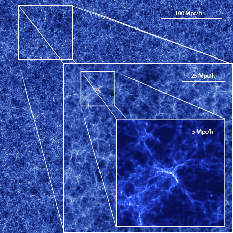
Figure 1: Environment of the most massive black hole at $z=8$ in BT (Left) and its descendant at $z=0$ in BTMassTracer (Right). The images show the dark matter density in a slice through the entire simulation (width $400h^{-1}Mpc$) and thickness 2 $h^{-1}Mpc$. In the left panel, the intensity and color of the pixels is representative the density of dark matter at each point. In the right panel, at lower redshift, the intensity is proportional to the density and the color scale indicates the gravitational potential.

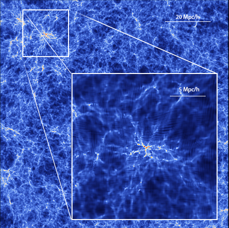
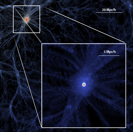
Figure 2: Environment : Descendant of the $z=8$ most massive FOF halo in a $100h^{-1}Mpc$ region at $z=8$ (Left) and $z=0$ (Right).

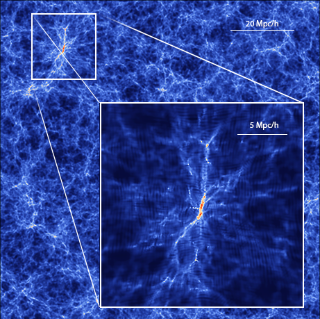
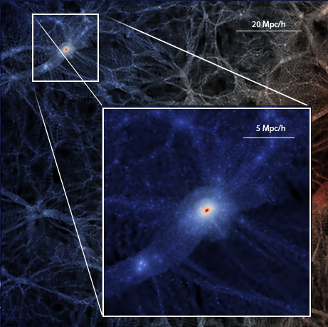
Figure 3: Environment : $z=0$ most massive FOF halo in a $100h^{-1}Mpc$ region at $z=8$ (Left) and $z=0$ (Right).

Before carrying out a statistical study of the descendants of high redshift quasars, we examine a few illustrative cases. First, we track the tracer of the most massive blackhole at $z=8$ based on the method described in Section 2 and identify the host halo at $z=0$. Figure 1 shows the distribution of dark matter in a slice through the simulation that includes the massive black hole at $z=8$ and its tracer at $z=0$. The slices plotted are 2 ${\rm h^{-1}Mpc}$ thick and in each case we also show zooms into a 100 ${\rm h^{-1}Mpc}$ wide and 20 ${\rm h^{-1}Mpc}$ wide subvolume. In order to highlight the variety of features present in the high and low density universe, we use a color scale in the $z=0$ panel which varies with the gravitational potential. We can see that, as expected, the density field is much more structured at redshift $z=0$ and visible filaments extend to larger scales. The quasar descendant inhabits an elliptical halo with projected minor and major axes with dimensions $\sim 1h^{-1}Mpc$ and $\sim 2h^{-1}Mpc$. Its mass is $4.92\times 10^{14}M_{\odot}$, comparable to a large galaxy group such as the NGC 1600 group (Thomas et al., 2016).It is connected to the surrounding large-scale structure by 5 obvious filaments at $z=0$, and at $z=8$ it appears to lie at the intersection of 3 filaments. The extent of the “protocluster” at $z=8$ visible in the zoomed panel is not much larger than the final cluster at $z=0$. This indicates that the 3 filament structures seen at $z=8$ must have collapsed, virialised and consequently erased by $z=0$. At $z=8$, the halo hosting the most massive black hole has a mass of $8.43\times 10^{11}M_{\odot}$ and its descendant is the $242^{nd}$ most massive halo at $z=0$.

We also trace the most massive halo at $z=8$ forward to $z=0$. This halo has a mass of $2.77\times 10^{12}M_{\odot}$ at $z=8$ and is about $3$ times more massive than the host of the most massive black hole. Its environment at these two redshifts is shown in Figure 2. The protocluster region at $z=8$ in this case is more spherically symmetric, and less filamentary than in Figure 1. These two objects are extreme, and this finding is counter to the trend seen on average by Di Matteo et al. (2017) that early quasars preferentially occur in regions with low tidal fields. At $z=0$ the halo that was the most massive at $z=8$ is now the $258^{th}$ most massive with a mass of $4.79\times 10^{14}M_{\odot}$, and appears more spherical than the quasar host descendant.

An alternative way to study these extreme objects is instead to track halos backwards in time. We have done this in Figure 3, where we show the most massive halo at $z=0$ and environment around its progenitor at $z=8$. In this case, the $z=0$ halo has a mass of $3.59\times 10^{15}M_{\odot}$, comparable to the Coma cluster. At $z=8$, it lies in a $\sim 6{\rm h^{-1}Mpc}$ filament, and the progenitor halo has a mass $1.25\times 10^{12}M_{\odot}$ ( $\sim 45\%$ of the mass of the most massive halo at $z=8$). Looking at the very top halos and black holes in mass as we have done in these three figures, we can see that they reside in obviously dense environments, and have similar halo masses. It is not clear however what happens to the bulk of the population- for example whether all early quasars have massive descendants, or conversely all the massive halos at $z=0$ hosted massive black holes at $z=8$. We can answer this by tracking a statistical sample of objects.

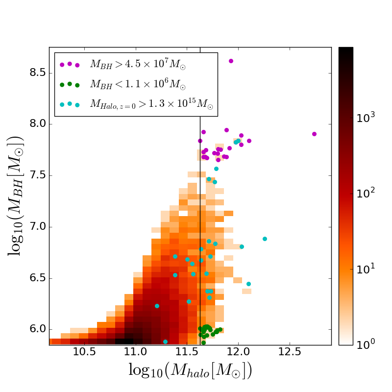
Figure 4: Two dimensional histogram of the logarithm of halo mass ($\log_{10}(M_{halo}[M_{\odot}])$) and the black hole mass ($\log_{10}(M_{BH}[M_{\odot}])$) in the BlueTides Hydrodynamic simulation at $z=8$. The 23 most massive black holes are shown by scatter points in purple, while the least massive blackholes are shown in green. We also show as cyan points, the blackholes in the progenitor halos of the most massive halos at $z=0$.

In Figure 4, we plot a two-dimensional histogram of halo mass and the corresponding black hole mass at $z=8$ in the BlueTides hydrodynamic simulation. The scatter points colored in magenta in the figure show the halos with black hole mass, $M_{BH}>4.5\times 10^{7}M_{\odot}$ which correspond to the 23 most massive black holes at $z=8$. We track these in the BlueTides MassTracer simulation. In a similar halo mass range, we also track an equal number of least massive black holes (shown as green points) in order to compare the properties of the descendants of the halos with massive quasars with those of halos whose black hole mass is much lower, around that of the seed black hole mass. While matching halos in the BT hydrodynamic and BTMassTracer simulation, we note that the halo mass is different in the matched halos due to baryonic effects and there can be differences, which are mostly within $20\%$.

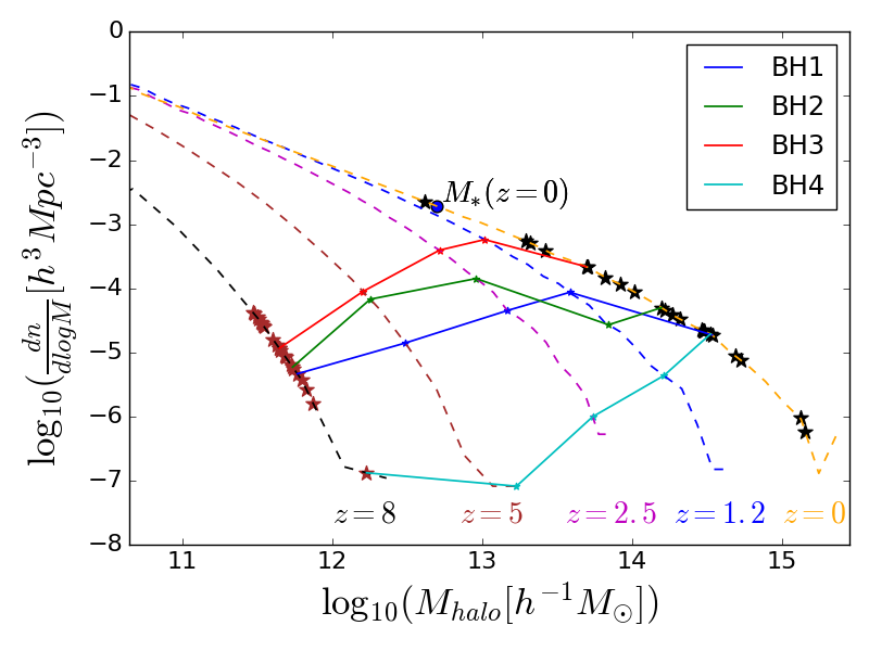
Figure 5: Left: Halo Mass function at $z=8,5,2.5,1.2,0$ and the location of the tracked hosts of the 4 most massive BH’s on the mass function. Right: Normalized histogram of the halo masses at $z=0$ of the descendants of the most massive black holes at $z=8$ compared with the histogram of most massive halos at $z=0$.

In the left panel of Figure 5, we plot the halo mass function of the dark matter halos at $z=8,5,2.5,1.2,0$. We also plot as points on the halo mass function at $z=8$ and $z=0$ the hosts of the most massive black hole tracer particles (corresponding to the purple points in Figure 4). We find that at redshift $z=0$, the halo masses are distributed over a wide range, compared to that at $z=8$. From the figure, we can therefore clearly see that the descendants of the most massive black holes at $z=8$ are not all the most massive halos at $z=0$. However, the descendants are still relatively massive halos with mass above $M_{*}=5.0\times 10^{12}h^{-1}M_{\odot}$ at $z=0$. The individual tracks for the halo masses of the four most massive black hole tracers are also shown in the figure. We can see that these objects approximately keep their rank order over all redshifts.

To further understand the distribution of the halo masses, we plot the normalized histogram of the host halo masses of the descendants of the $z=8$ massive black holes, compared with the 23 most massive halos at $z=0$ in the right panel of Figure 5. While the most massive halos are distributed above $3.2\times 10^{14}h^{-1}M_{\odot}$ with a peak in the distribution at $\sim 1.8\times 10^{15}h^{-1}M_{\odot}$, the quasar descendants have a peak distribution in the mass at $\sim 2.24\times 10^{14}h^{-1}M_{\odot}$. These 23 most massive halos and 23 quasar descendants have a space density of $4\times 10^{-7}{\rm h^{3}Mpc^{-3}}$. The massive halos are all Coma-like objects, whereas the quasar descendants have masses an order of magnitude smaller, comparable to galaxy groups with a space density $\sim 10^{-5}{\rm h^{3}Mpc^{-3}}$.

We can similarly compare the distribution of halo masses for the descendants of the least massive black holes at $z=8$ with those of the most massive ones, whose halo masses at $z=8$ are in the similar mass range. These are the green points in Figure 4. Tracking forwards to $z=0$, we show the normalized histogram of the halo masses for the descendants of the least massive and the most massive black holes in the left panel of Figure 6. We can clearly see that the distribution of halo masses are in similar range in both cases. Based on a KS-test, we have verified that the distributions are statistically consistent with each other (see numerical values in the figure caption). This is the case even though the black hole masses at $z=8$ in the two subsamples are different by about two orders of magnitude.

We have seen that after controlling for the effect of halo mass, high redshift quasars do not have overly massive descendants. An interesting related question is whether the most massive halos at $z=0$ were hosting overly massive black holes at high redshift. In order to answer this, we need to find the $z=8$ black hole masses (in the BlueTides run) of the most massive halos (in the BTMassTracer run) at $z=0$. First, we identify the tracers of the black hole particles at $z=8$ which are in the 23 most massive halos at $z=0$. This is done by identifying halos such that the most bound particle in these halos at $z=8$ is present in the corresponding most massive halos at $z=0$. By matching these halos in the BTMassTracer simulation at $z=8$ with that of the hydrodynamic simulation, we can identify the black hole masses at $z=8$, whose descendants are the most massive halos at $z=0$.

In Figure 4, we show these black hole masses as cyan points. We can see that they are spread throughout the range of masses plotted, with most lying in between the most massive ($\sim 10^{8}M_{\odot}$) and the least massive $\sim 10^{6}M_{\odot}$. The normalized histograms of these black hole masses are plotted in the right panel of Figure 6, compared with the distribution of the most massive black holes. From the figure, we can see that the most massive halos at $z=0$ are the descendants of the black holes mostly with masses less than $10^{7}M_{\odot}$ and the peak in their mass distribution is at $\sim 3.2\times 10^{6}M_{\odot}$. The most massive black holes have masses above $10^{7}M_{\odot}$ with a peak in the distribution at $\sim 10^{8}M_{\odot}$. This result is consistent with our discussion earlier that the descendants of the most massive black holes at $z=8$ are not among the the most massive halos.

Finally, for a given halo mass at $z=0$, we can make predictions about its black hole mass at $z=8$ from our analysis. In Figure 7, we plot the probability that the black hole mass at $z=8$ falls within certain mass bins. We choose $7.1\times 10^{5}M_{\odot}\leq M_{BH}<1.9\times 10^{6}M_{\odot}$, $1.9\times 10^{6}M_{\odot}\leq M_{BH}<5.1\times 10^{6}M_{\odot}$, $5.1\times 10^{6}M_{\odot}\leq M_{BH}<1.4\times 10^{7}M_{\odot}$, $1.4\times 10^{7}M_{\odot}\leq M_{BH}<3.7\times 10^{7}M_{\odot}$ or $\geq 3.7\times 10^{7}M_{\odot}$ for a given halo mass at $z=0$. We find that the most massive halos at $z=0$, are most likely to be descendants of $z=8$ black holes in the mass range between $10^{6}-1.4\times 10^{7}M_{\odot}$ , when compared to the massive black holes with $M_{BH}>3.7\times 10^{7}M_{\odot}$ which is consistent with the results shown in Figure 6. However, as noted earlier, the descendants of most massive black holes are relatively massive with $M_{Halo,z=0}>M_{*,z=0}$ and the probability that halos with masses less than $10^{13}h^{-1}M_{\odot}$ at $z=0$ are descendants of massive black holes at $z=8$ is very small.

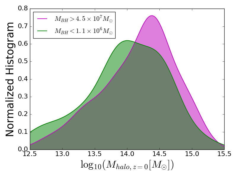
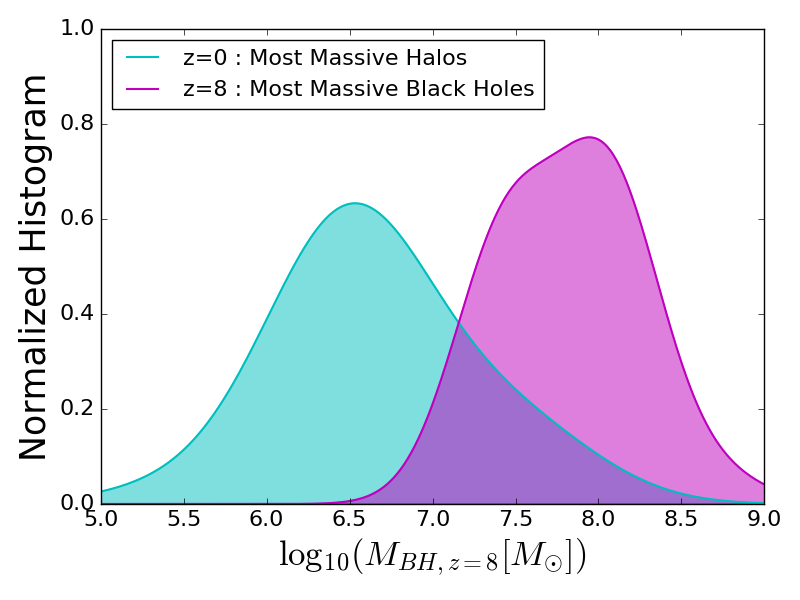
Figure 6: Left: Normalized histogram of the halo masses at $z=0$ of the descendants of the most massive black holes ($M_{BH}>10^{7.653}M_{\odot}$)and the least massive black holes ($M_{BH}<10^{6.031}M_{\odot}$) at $z=8$. Note : KS-test statistic shows that the distributions are similar with $\alpha=0.26$ and $p$-value = $0.36$. Right: Normalized histogram of the black hole masses of the most massive black holes at $z=8$ and the black holes whose descendants are the most massive halos at $z=0$.

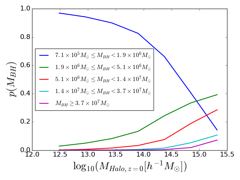
Figure 7: Likelihood of the black hole mass of the halo at $z=8$, $M_{BH}$ is with in the range, $7.1\times 10^{5}M_{\odot}\leq M_{BH}<1.9\times 10^{6}M_{\odot}$, $1.9\times 10^{6}M_{\odot}\leq M_{BH}<5.1\times 10^{6}M_{\odot}$, $5.1\times 10^{6}M_{\odot}\leq M_{BH}<1.4\times 10^{7}M_{\odot}$, $1.4\times 10^{7}M_{\odot}\leq M_{BH}<3.7\times 10^{7}M_{\odot}$ or $\geq 3.7\times 10^{7}M_{\odot}$ given the halo mass of the descendant at $z=0$.

4 Conclusions

In this paper, we have used the BlueTides MassTracer simulation, a dark matter-only realization of the BlueTides hydrodynamical simulation (Feng et al., 2016) to trace the host halo descendants of the first, rare massive black hole/quasars to the present day. Due to its large volume and high resolution it is currently prohibitive (even on the largest machines) to run BlueTides (with hydrodynamics and sub-grid physics of galaxy formation) significantly beyond high redshift. We match the halos in BlueTides hydrodynamic and the BT MassTracer simulation which are evolved from the same initial conditions at $z=8$. The most bound particles in the matched halos of the dark matter-only simulation are tracked to $z=0$ to identify the descendants of the most massive black holes.

Our main finding is that the rare quasars with the most massive black holes do not have the most massive low redshift descendants. The BTMassTracer simulation is large enough that it contains several hundred galaxy clusters with masses $\sim 10^{15}M_{\odot}$ at redshift $z=0$. These objects however do not contain these quasar blackholes, which instead reside in galaxy groups with masses $\sim 10^{14}M_{\odot}$. We further find that for similar range of halo masses at $z=8$, the halo masses of the low-redshift descendants of the least massive high-redshift black holes at $z=0$ have a distribution similar to those of the descendants of most massive high-redshift black holes. Consistent with our results, Fanidakis et al. (2013) and Uchiyama et al. (2017) find that the most luminous quasars do not live in the most massive halos. Further, Trainor & Steidel (2012) find that the most luminous quasars exist in similar environments when compared with that of their less luminous counterparts. It is also to be noted that Thomas et al. (2016) report the discovery of a luminous blackhole whose descendant is found in a relatively isolated galaxy.

We also find that the $z=8$ progenitors of the most massive halos at $z=0$ do not necessarily host the most massive black holes. We determined the black hole masses, by identifying the $z=8$ progenitors of the massive halos at $z=0$ in the BT MassTracer simulation, which are matched to the $z=8$ halos in the BlueTides hydrodynamic simulation. The black hole masses of these progenitors are distributed over a range of masses from $10^{6-8}M_{\odot}$ with the most likely black hole mass being about $3.2\times 10^{6}M_{\odot}$. Finally, we estimate the likelihood that the $z=8$ progenitors will host black holes of a certain mass, given the halo mass at $z=0$. We find that for massive halos with masses above $10^{15}h^{-1}M_{\odot}$ at $z=0$, there is only a $7\%$ probability of its progenitor hosting a black hole with $M_{BH}>3.7\times 10^{7}M_{\odot}$ at $z=8$. The black holes are most likely to be in the mass range, $2\times 10^{6}-5\times 10^{6}M_{\odot}$, where the likelihood is about $40\%$.

As we have mentioned, our result is not surprising considering observational evidence that quasars may populate halos which are not the most massive. It is however counter to the simplest possible scenario, that high peaks form high redshift quasars and continue to evolve into the highest peaks at $z=0$. This may indicate that abundance matching techniques used in large-scale structure and galaxy property studies may not work well in the context of quasars. This is consistent with the finding that other environmental properties, such as tidal field strength appear to be important in the formation of these early supermassive black holes ( Di Matteo et al. (2017)). Trenti & Stiavelli (2007) showed using simulations that the material from the $10^{6}h^{-1}M_{\odot}$ mass halos hosting the first stars does not end up at later times ($z=6$ in that case) in the halos hosting bright quasars, but instead spans a range of environments. Our study can be viewed as an extension of this work to lower redshift, although we find that galaxy groups are the most likely host at $z=0$. Observational signatures of this could in principle include a deficit of old stars in groups at $z=0$ due to strong early episodes of quasar feedback.

References

- Barber et al. (2016) Barber C., Schaye J., Bower R. G., Crain R. A., Schaller M., Theuns T., 2016, MNRAS, 460, 1147
- Di Matteo et al. (2005) Di Matteo T., Springel V., Hernquist L., 2005, Nature, 433, 604
- Di Matteo et al. (2017) Di Matteo T., Croft R. A. C., Feng Y., Waters D., Wilkins S., 2017, MNRAS, 467, 4243
- Fanidakis et al. (2013) Fanidakis N., Macciò A. V., Baugh C. M., Lacey C. G., Frenk C. S., 2013, MNRAS, 436, 315
- Feng et al. (2016) Feng Y., Di-Matteo T., Croft R. A., Bird S., Battaglia N., Wilkins S., 2016, MNRAS, 455, 2778
- Hinshaw et al. (2013) Hinshaw G., et al., 2013, ApJS, 208, 19
- Hopkins (2013) Hopkins P. F., 2013, MNRAS, 428, 2840
- Katz et al. (1996) Katz N., Weinberg D. H., Hernquist L., 1996, ApJS, 105, 19
- Krumholz & Gnedin (2011) Krumholz M. R., Gnedin N. Y., 2011, ApJ, 729, 36
- Ma et al. (2014) Ma C.-P., Greene J. E., McConnell N., Janish R., Blakeslee J. P., Thomas J., Murphy J. D., 2014, ApJ, 795, 158
- McConnell et al. (2011) McConnell N. J., Ma C.-P., Gebhardt K., Wright S. A., Murphy J. D., Lauer T. R., Graham J. R., Richstone D. O., 2011, Nature, 480, 215
- Mortlock et al. (2011) Mortlock D. J., et al., 2011, Nature, 474, 616
- Okamoto et al. (2010) Okamoto T., Frenk C. S., Jenkins A., Theuns T., 2010, MNRAS, 406, 208
- Read et al. (2010) Read J. I., Hayfield T., Agertz O., 2010, MNRAS, 405, 1513
- Springel & Hernquist (2003) Springel V., Hernquist L., 2003, MNRAS, 339, 289
- Thomas et al. (2016) Thomas J., Ma C.-P., McConnell N. J., Greene J. E., Blakeslee J. P., Janish R., 2016, Nature, 532, 340
- Trainor & Steidel (2012) Trainor R. F., Steidel C. C., 2012, ApJ, 752, 39
- Trenti & Stiavelli (2007) Trenti M., Stiavelli M., 2007, ApJ, 667, 38
- Uchiyama et al. (2017) Uchiyama H., et al., 2017, preprint, (arXiv:1704.06050)
- Vogelsberger et al. (2013) Vogelsberger M., Genel S., Sijacki D., Torrey P., Springel V., Hernquist L., 2013, MNRAS, 436, 3031
- Vogelsberger et al. (2014) Vogelsberger M., et al., 2014, MNRAS, 444, 1518
- Wu et al. (2015) Wu X.-B., et al., 2015, Nature, 518, 512