Quantum renormalization group of XY model in two-dimensions

Abstract

We investigate entanglement and quantum phase transition (QPT) in a two-dimensional Heisenberg anisotropic spin-1/2 XY model, using quantum renormalization group method (QRG) on a square lattice of $N\times N$ sites. The entanglement through geometric average of concurrences is calculated after each step of the QRG. We show that the concurrence achieves a non zero value at the critical point more rapidly as compared to one-dimensional case. The relationship between the entanglement and the quantum phase transition is studied. The evolution of entanglement develops two saturated values corresponding to two different phases. We compute the first derivative of the concurrence, which is found to be discontinuous at the critical point $\gamma=0$, and indicates a second-order phase transition in the spin system. Further, the scaling behaviour of the system is investigated by computing the first derivative of the concurrence in terms of the system size.

I INTRODUCTION

In quantum systems, entanglement is a resource that reveals the difference between classical and quantum physics xydm1 . Its role has been considered very vital to implement the quantum information tasks in innovative ways like in quantum computations, quantum cryptography and quantum teleportation etc. NC 2000 . In ecent years, the study of entanglement in strongly correlated systems have attracted much more attention vedral intro(1) ; vedral intro(3) because it can describe not only the information processing through correlation of spins vedral intro(7) but also the critical phenomenon, quantum phase transition (QPT) vedral intro(2) . Therefore, the quantum entanglement is considered as the common ground between the quantum information theory (QIT) and the condensed matter physics xydm8 ; Langari xxz 1 . Recently, much efforts have been devoted to the study of Heisenberg spin models, especially, one dimensional spin models are the most explored area of research, as these systems are exactly solvable and give quantitative results xy3 ; xy4 ; xy5 ; ising ; xxz ; xxzdm ; xy ; xydm ; vedral spin1/2(1) ; vedral spin 1/2(2) .

In higher dimensions, almost all the analysis of entanglement and the QPT were made through numerical simulations NS1 ; NS2 . Whereas the study of the phase diagram was also carried out PD1 ; PD2 ; PD3 . Using Monte Carlo simulations, concurrence was considered as an entanglement measure in two-dimensional XY and XXZ models NS1 ; NS2 . In the d-dimension pair wise entanglement was studied in XXZ model NS3 ; NS4  Concurrence was used to calculate the quantum entanglement in the spin$-1/2$ ladder with four spins ring exchange by exact diagonalization method NS5 .

The density-matrix renormalization group method is a leading numerical technique useful in exploring ground state properties for many body interactions in lower dimensions xydm16 ; xydm17 ; xydm18 ; xydm19 . Alongside, quantum renormalization group method (QRG) is another technique which deals with large size systems analytically. At low temperatures behavior of the spin systems effect their quantum nature due to quantum fluctuations. At these temperatures, ground states can be used to measure entanglement through density matrix evaluation, where the non analytical behavior of the derivative of entanglement explains the phenomenon of QPT xxz ; xxzdm ; xy ; xydm . Such approaches can be implemented in the QRG method.

The QRG method was used to solve exactly the one dimensional Ising, XXZ and XY models ising ; xxz ; xxzdm ; xy ; xydm . Where it was found that the nearest neighbors interaction exhibits the QPT near the critical point. For a deeper insight, the next nearest neighbors interaction was studied in XXZ model xydm30 ; xydm31 . The RG method was also used in the one dimensional Ising and XYZ models in the presence of magnetic field ising ; xyz .The Jordan Wigner transformation was used to solve the Ising model exactly, where it was found that near critical point, this model exhibits the maximum value of entanglement for the second nearest neighbors vedral intro(1) . It was analyzed that in thermodynamic limit the entanglement of ground state of mutually interacting spin-1/2 particles in a magnetic field shows cusp like singularities exactly at the critical point vedral intro(1) . The QRG method in two dimensional spin systems is a step forward for the better understanding and answering the open questions like computational complexity of finding the ground states, ground state properties, energy spectrum, correlation length, criticality, quantum phase transition and their connection with entanglement. Analogous to Kadanoff’s block renormalization group approach in one-dimensional spin systems xy30 , we apply to two-dimensional spin systems by dividing the square lattice of spins into blocks of odd number of spins, which span the whole lattice.

The rest of the paper is arranged as follow. In Sec. II, we present the model of the system and describe the mathematical formalism to calculate the renormalized coupling constant and anisotropic coefficients. The effective Hamiltonian of the system is obtained in terms of renormalized constants. In Sec. III we investigate the block-block entanglement and its non analytical behavior which is related to the QPT. We also study the scaling behavior in this context. The results are summarized in Sec. IV.

II QUANTUM RENORMALIZATION OF XY MODEL IN TWO-DIMENSIONS

Kadanoff block approach was used in the past to study the QRG method in one-dimensional spin models xy3 ; xy4 ; xy5 ; ising ; xxz ; xxzdm ; xy ; xydm . In this approach the fixed point is achieved after number of iterations by virtue of reduction of degrees of freedom. We extend this very idea and implement it on a two-dimensional square lattice of spins, in which the whole lattice is spanned by square blocks, each consisting of five spins (FIG. 1), with one spin at the center and four at the corners. Using this model we obtain the renormalized parameters producing the effective Hamiltonian similar to the original one. The Hamiltonian of a two dimensional Heisenberg XY model represented by the square lattice of $N\times N$ spins can be written as,

$$H(J,\gamma)=\frac{J}{4}\sum_{i=1}^{N}\sum_{j=1}^{N}((1+\gamma)(\sigma_{i,j}^{x}\sigma_{i+1,j}^{x}+\sigma_{i,j}^{x}\sigma_{i,j+1}^{x})+(1-\gamma)(\sigma_{i,j}^{y}\sigma_{i+1,j}^{y}+\sigma_{i,j}^{y}\sigma_{i,j+1}^{y})),$$ (1)

where $J$ is the exchange coupling constant, $\gamma$ is the anisotropy parameter and $\sigma^{x},\sigma^{y}$ are the Pauli matrices. Depending on the values of $\gamma$ the model reduces to different classes such as $XX$ model for $\gamma=0,$ Ising model for $\gamma=1$ and Ising universality class for $0<\gamma\leq 1$ xy22 .

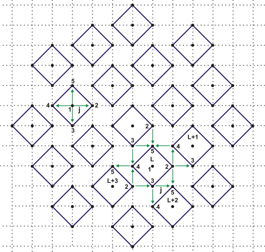
Figure 1: (Color online) 2-dimensional square lattice is depicted by considering each block of five spins.

We begin by dividing the total Hamiltonian into two parts as

$$H=H^{B}+H^{BB},$$ (2)

where $H^{B}$ and $H^{BB}$ are the block and the interblock Hamiltonians respectively. The explicit form of these Hamiltonians can be written as

$$H^{B} =\frac{J}{4}\sum\limits_{L}^{N/5}((1+\gamma)(\sigma_{L,1}^{x}\sigma_{L,2}^{x}+\sigma_{L,1}^{x}\sigma_{L,3}^{x}+\sigma_{L,1}^{x}\sigma_{L,4}^{x}+\sigma_{L,1}^{x}\sigma_{L,5}^{x})$$

$$+(1-\gamma)(\sigma_{L,1}^{y}\sigma_{L,2}^{y}+\sigma_{L,1}^{y}\sigma_{L,3}^{y}+\sigma_{L,1}^{y}\sigma_{L,4}^{y}+\sigma_{L,1}^{y}\sigma_{L,5}^{y})),$$ (3)

and

$$H^{BB} =\sum\limits_{L}^{N/5}\frac{J}{4}((1+\gamma)(\sigma_{L,2}^{x}\sigma_{L+1,3}^{x}+\sigma_{L,2}^{x}\sigma_{L+1,4}^{x}+\sigma_{L,2}^{x}\sigma_{L+2,5}^{x}+\sigma_{L,3}^{x}\sigma_{L+2,4}^{x}$$

$$+\sigma_{L,3}^{x}\sigma_{L+2,5}^{x}+\sigma_{L,4}^{x}\sigma_{L+3,5}^{x})+(1-\gamma)(\sigma_{L,2}^{y}\sigma_{L+1,3}^{y}+\sigma_{L,2}^{y}\sigma_{L+1,4}^{y}$$

$$+\sigma_{L,2}^{y}\sigma_{L+2,5}^{y}+\sigma_{L,3}^{y}\sigma_{L+2,4}^{y}+\sigma_{L,3}^{y}\sigma_{L+2,5}^{y}+\sigma_{L,4}^{y}\sigma_{L+3,5}^{y})),$$ (4)

Whereas the $L$th block Hamiltonian can be written as

$$H_{L}^{B} =\frac{J}{4}((1+\gamma)(\sigma_{L,1}^{x}\sigma_{L,2}^{x}+\sigma_{L,1}^{x}\sigma_{L,3}^{x}+\sigma_{L,1}^{x}\sigma_{L,4}^{x}+\sigma_{L,1}^{x}\sigma_{L,5}^{x})$$

$$+(1-\gamma)(\sigma_{L,1}^{y}\sigma_{L,2}^{y}+\sigma_{L,1}^{y}\sigma_{L,3}^{y}+\sigma_{L,1}^{y}\sigma_{L,4}^{y}+\sigma_{L,1}^{y}\sigma_{L,5}^{y})).$$ (5)

The interblock interactions are shown by direction of arrows in FIG. 1, which is mathematically represented by Eq. 4. We choose block of odd spins which in turn produces degenerate eigenvalues for the ground state and makes it possible to construct the projection operator in the renamed basis of the ground state. In terms of matrix product states xy29 , the solution i.e., the eigenvalues and the eigenvectors for the single block Hamiltonian, can be obtained. Therefore, the degenerate lowest energy can be written as

$$E_{0}=-\frac{1}{2}J\sqrt{5+5\gamma^{2}+\alpha_{1}},$$ (6)

and the corresponding states in terms of eigenstates $\left|\uparrow\right\rangle$, $\left|\downarrow\right\rangle$ of $\sigma^{z}$ are

$$\left|\phi_{0}^{1}\right\rangle =\gamma_{1}(\left|\uparrow\uparrow\uparrow\uparrow\downarrow\right\rangle+\left|\uparrow\uparrow\uparrow\downarrow\uparrow\right\rangle+\left|\uparrow\uparrow\downarrow\uparrow\uparrow\right\rangle+\left|\uparrow\downarrow\uparrow\uparrow\uparrow\right\rangle)$$

$$+\gamma_{2}(\left|\uparrow\uparrow\downarrow\downarrow\downarrow\right\rangle+\left|\uparrow\downarrow\uparrow\downarrow\downarrow\right\rangle+\left|\uparrow\downarrow\downarrow\uparrow\downarrow\right\rangle+\left|\uparrow\downarrow\downarrow\downarrow\uparrow\right\rangle)$$

$$+\gamma_{3}\left|\downarrow\uparrow\uparrow\uparrow\uparrow\right\rangle+\gamma_{4}(\left|\downarrow\uparrow\uparrow\downarrow\downarrow\right\rangle+\left|\downarrow\uparrow\downarrow\uparrow\downarrow\right\rangle+\left|\downarrow\uparrow\downarrow\downarrow\uparrow\right\rangle$$

$$+\left|\downarrow\downarrow\uparrow\uparrow\downarrow\right\rangle+\left|\downarrow\downarrow\uparrow\downarrow\uparrow\right\rangle+\left|\downarrow\downarrow\downarrow\uparrow\uparrow\right\rangle)+\gamma_{5}\left|\downarrow\downarrow\downarrow\downarrow\downarrow\right\rangle,$$ (7)

and

$$\left|\phi_{0}^{2}\right\rangle =\gamma_{6}\left|\uparrow\uparrow\uparrow\uparrow\uparrow\right\rangle+\gamma_{7}(\left|\uparrow\uparrow\uparrow\downarrow\downarrow\right\rangle+\left|\uparrow\uparrow\downarrow\uparrow\downarrow\right\rangle+\left|\uparrow\uparrow\downarrow\downarrow\uparrow\right\rangle$$

$$+\left|\uparrow\downarrow\uparrow\uparrow\downarrow\right\rangle+\left|\uparrow\downarrow\uparrow\downarrow\uparrow\right\rangle+\left|\uparrow\downarrow\downarrow\uparrow\uparrow\right\rangle)+\gamma_{8}\left|\uparrow\downarrow\downarrow\downarrow\downarrow\right\rangle$$

$$+\gamma_{9}(\left|\downarrow\uparrow\uparrow\uparrow\downarrow\right\rangle+\left|\downarrow\uparrow\uparrow\downarrow\uparrow\right\rangle+\left|\downarrow\uparrow\downarrow\uparrow\uparrow\right\rangle+\left|\downarrow\downarrow\uparrow\uparrow\uparrow\right\rangle)$$

$$+\gamma_{10}(\left|\downarrow\uparrow\downarrow\downarrow\downarrow\right\rangle+\left|\downarrow\downarrow\uparrow\downarrow\downarrow\right\rangle+\left|\downarrow\downarrow\downarrow\uparrow\downarrow\right\rangle+\left|\downarrow\downarrow\downarrow\downarrow\uparrow\right\rangle).$$ (8)

Expressions for the $\ \alpha_{1},$ and the $\ \gamma_{i}$’$s$ in terms of the $\gamma$ are given in the appendix.

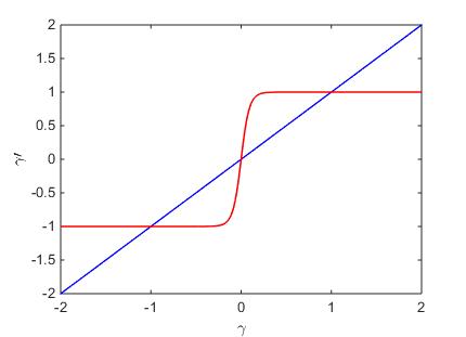
Figure 2: (Color online) $\gamma^{\prime}$ is plotted against the anisotropic parameter $\gamma$ for Eq. 17 (red) and for $\gamma=\gamma^{\prime}$ (blue). The values of $\gamma=0,\pm 1$ provide the solution for $\gamma=\gamma^{\prime}$.

Our aim is to construct the effective Hamiltonian $H^{eff}$ in the renormalized subspace by finding the renormalized coupling constant and anisotropy parameter from the projection operators $P_{0}$. For which the projection operators $P_{0}$ are obtained from the degenerate ground state eigenvectors of the block Hamiltonian $H^{B}$. The effective Hamiltonian is related to the original Hamiltonian through xy30

$$H^{eff}=P_{0}^{{\dagger}}HP_{0},$$ (9)

where $P_{0}^{{\dagger}}$ is the Hermitian adjoint of $P_{0}$. Using the perturbative method, we consider only the first order correction term. The effective Hamiltonian is given by xxz ; xy

$$H^{eff} =H_{0}^{eff}+H_{1}^{eff}$$

$$=P_{0}^{{\dagger}}H^{B}P_{0}+P_{0}^{{\dagger}}H^{BB}P_{0}.$$ (10)

In terms of the renamed states of $L$th block, the projection operator $P_{0}^{L}$ is defined as xxz ; xy

$$P_{0}^{L}=\left|\Uparrow\right\rangle_{L}\left\langle\phi_{0}^{1}\right|+\left|\Downarrow\right\rangle_{L}\left\langle\phi_{0}^{2}\right|,$$ (11)

where $P_{0}$ can be described in product form as

$$P_{0}=\prod\limits_{L}^{N/5}P_{0}^{L},$$ (12)

and $\left|\Uparrow\right\rangle_{L}$ and $\left|\Downarrow\right\rangle_{L}$ are the simple qubits of $L$th block to represent effective site degrees of freedom. The renormalization of the Pauli matrices is given as

$$P_{0}^{L}\text{ }\sigma_{i,L}^{\varepsilon}\text{ }P_{0}^{L}=\eta_{i}^{\varepsilon}\text{ }\acute{\sigma}_{L}^{\varepsilon}\text{ \ \ \ \ }(i=1,2,3,4,5\text{ };\text{ }\varepsilon=x,y),$$ (13)

where

$$\eta_{1}^{x} = 4\gamma_{10}\gamma_{2}+\gamma_{3}\gamma_{6}+6\gamma_{4}\gamma_{7}+\gamma_{5}\gamma_{8}+4\gamma_{1}\gamma_{9},$$

$$\eta_{2}^{x} = \eta_{3}^{x}=\eta_{4}^{x}=\eta_{5}^{x}$$

$$= \gamma_{10}(3\gamma_{4}+\gamma_{5})+3\gamma_{2}\gamma_{7}+\gamma_{1}(\gamma_{6}+3\gamma_{7})+\gamma_{2}\gamma_{8}+\gamma_{9}(\gamma_{3}-3\gamma_{4}),$$

$$\eta_{1}^{y} = 4\gamma_{10}\gamma_{2}-\gamma_{3}\gamma_{6}-6\gamma_{4}\gamma_{7}-\gamma_{5}\gamma_{8}+4\gamma_{1}\gamma_{9},$$

$$\eta_{2}^{y} = \eta_{3}^{y}=\eta_{4}^{y}=\eta_{5}^{y}$$ (14)

$$= \gamma_{10}(3\gamma_{4}-\gamma_{5})-3\gamma_{2}\gamma_{7}+\gamma_{1}(-\gamma_{6}+3\gamma_{7})+\gamma_{2}\gamma_{8}+\gamma_{9}(\gamma_{3}+3\gamma_{4}).$$

The effective Hamiltonian of the renormalized two dimensional spins surface is mapped on to the original Hamiltonian with renormalized coupling parameters, i.e.,

$$H^{eff}=\frac{\acute{J}}{4}\sum_{p=1}^{N/5}\sum_{q=1}^{N/5}((1+\acute{\gamma})(\sigma_{p,q}^{x}\sigma_{p+1,q}^{x}+\sigma_{p,q}^{x}\sigma_{p,q+1}^{x})+(1-\acute{\gamma})(\sigma_{p,q}^{y}\sigma_{p+1,q}^{y}+\sigma_{p,q}^{y}\sigma_{p,q+1}^{y})),$$ (15)

where

$$\acute{J} =j(\gamma_{10}^{2}(9\gamma_{4}^{2}+6\gamma\gamma_{4}\gamma_{5}+\gamma_{5}^{2})+9\gamma_{2}^{2}\gamma_{7}^{2}+\gamma_{1}^{2}(\gamma_{6}^{2}+6\gamma\gamma_{6}\gamma_{7}+9\gamma_{7}^{2})+6\gamma\gamma_{2}^{2}\gamma_{7}\gamma_{8}+\gamma_{2}^{2}\gamma_{8}^{2}$$

$$+6\gamma\gamma_{2}\gamma_{3}\gamma_{7}\gamma_{9}+18\gamma_{2}\gamma_{4}\gamma_{7}\gamma_{9}+2\gamma_{2}\gamma_{3}\gamma_{8}\gamma_{9}+6\gamma\gamma_{2}\gamma_{4}\gamma_{8}\gamma_{9}+\gamma_{3}^{2}\gamma_{9}^{2}+6\gamma\gamma_{3}\gamma_{4}\gamma_{9}^{2}$$

$$+9\gamma_{4}^{2}\gamma_{9}^{2}+2\gamma_{1}(\gamma_{2}(3\gamma_{7}(3\gamma\gamma_{7}+\gamma_{8})+\gamma_{6}(3\gamma_{7}+\gamma\gamma_{8}))+(\gamma\gamma_{3}\gamma_{6}+3\gamma_{4}\gamma_{6}+3\gamma_{3}\gamma_{7}$$

$$+9\gamma\gamma_{4}\gamma_{7})\gamma_{9})+2\gamma_{10}(\gamma_{1}(\gamma_{5}\gamma_{6}+9\gamma_{4}\gamma_{7})+\gamma(9\gamma_{2}\gamma_{4}\gamma_{7}+3\gamma_{1}(\gamma_{4}\gamma_{6}+\gamma_{5}\gamma_{7})$$

$$+\gamma_{2}\gamma_{5}\gamma_{8}+9\gamma_{4}^{2}\gamma_{9}+\gamma_{3}\gamma_{5}\gamma_{9})+3(\gamma_{2}(\gamma_{5}\gamma_{7}+\gamma_{4}\gamma_{8})+\gamma_{4}(\gamma_{3}+\gamma_{5})\gamma_{9}))),$$ (16)

and

$$\acute{\gamma} =(2(3\gamma_{10}\gamma_{4}+3\gamma_{1}\gamma_{7}+\gamma_{2}\gamma_{8}+\gamma_{3}\gamma_{9})(\gamma_{10}\gamma_{5}+\gamma_{1}\gamma_{6}+3\gamma_{2}\gamma_{7}+3\gamma_{4}\gamma_{9})+\gamma(\gamma_{10}^{2}(9\gamma_{4}^{2}$$

$$+\gamma_{5}^{2})+9\gamma_{2}^{2}\gamma_{7}^{2}+\gamma_{1}^{2}(\gamma_{6}^{2}+9\gamma_{7}^{2})+\gamma_{2}^{2}\gamma_{8}^{2}+18\gamma_{2}\gamma_{4}\gamma_{7}\gamma_{9}+2\gamma_{2}\gamma_{3}\gamma_{8}\gamma_{9}+\gamma_{3}^{2}\gamma_{9}^{2}+9\gamma_{4}^{2}\gamma_{9}^{2}$$

$$+6\gamma_{1}(\gamma_{2}\gamma_{7}(\gamma_{6}+\gamma_{8})+(\gamma_{4}\gamma_{6}+\gamma_{3}\gamma_{7})\gamma_{9})+2\gamma_{10}(\gamma_{1}(\gamma_{5}\gamma_{6}+9\gamma_{4}\gamma_{7})+3(\gamma_{2}(\gamma_{5}\gamma_{7}$$

$$+\gamma_{4}\gamma_{8})+\gamma_{4}(\gamma_{3}+\gamma_{5})\gamma_{9}))))/(\gamma_{10}^{2}(9\gamma_{4}^{2}+6\gamma\gamma_{4}\gamma_{5}+\gamma_{5}^{2})+9\gamma_{2}^{2}\gamma_{7}^{2}+\gamma_{1}^{2}(\gamma_{6}^{2}+6\gamma\gamma_{6}\gamma_{7}$$

$$+9\gamma_{7}^{2})+6\gamma\gamma_{2}^{2}\gamma_{7}\gamma_{8}+\gamma_{2}^{2}\gamma_{8}^{2}+6\gamma\gamma_{2}\gamma_{3}\gamma_{7}\gamma_{9}+18\gamma_{2}\gamma_{4}\gamma_{7}\gamma_{9}+2\gamma_{2}\gamma_{3}\gamma_{8}\gamma_{9}+6\gamma\gamma_{2}\gamma_{4}\gamma_{8}\gamma_{9}$$

$$+\gamma_{3}^{2}\gamma_{9}^{2}+6\gamma\gamma_{3}\gamma_{4}\gamma_{9}^{2}+9\gamma_{4}^{2}\gamma_{9}^{2}+2\gamma_{1}(\gamma_{2}(3\gamma_{7}(3\gamma\gamma_{7}+\gamma_{8})+\gamma_{6}(3\gamma_{7}+\gamma\gamma_{8}))+(\gamma\gamma_{3}\gamma_{6}$$

$$+3\gamma_{4}\gamma_{6}+3\gamma_{3}\gamma_{7}+9\gamma\gamma_{4}\gamma_{7})\gamma_{9})+2\gamma_{10}(\gamma_{1}(\gamma_{5}\gamma_{6}+9\gamma_{4}\gamma_{7})+\gamma(9\gamma_{2}\gamma_{4}\gamma_{7}+3\gamma_{1}(\gamma_{4}\gamma_{6}$$

$$+\gamma_{5}\gamma_{7})+\gamma_{2}\gamma_{5}\gamma_{8}+9\gamma_{4}^{2}\gamma_{9}+\gamma_{3}\gamma_{5}\gamma_{9})+3(\gamma_{2}(\gamma_{5}\gamma_{7}+\gamma_{4}\gamma_{8})+\gamma_{4}(\gamma_{3}+\gamma_{5})\gamma_{9}))).$$ (17)

By solving the Eq. 17 for $\gamma=\acute{\gamma}$, we get the solutions $\gamma=0,\pm 1$ as shown in FIG. 2. The model corresponds to the spin fluid phase for $\gamma\rightarrow 0$ which is called the XX model and it corresponds to Ising like phase for $\gamma\rightarrow 1$or $-1.$ It indicates that there lies a phase boundary which separates the two phases.

III STUDY OF ENTANGLEMENT

We analyze the entanglement by computing the bipartite concurrence of the interaction between different interblock spins by using the ground state density matrix. We compute the geometric average of the all possible bipartite concurrences. The pure density matrix can be written as,

$$\rho=\left|\phi_{0}^{1}\right\rangle\left\langle\phi_{0}^{1}\right|,$$ (18)

where $\left|\phi_{0}^{1}\right\rangle$ is one of the ground state as given in Eq. 7. We calculate the reduced density matrices $\rho_{23},\rho_{24,}\rho_{25,}\rho_{34,}\rho_{35,}\rho_{45,}$ by taking the multiple traces and then the bipartite concurrences are worked out. For the entanglement measurement we compute the geometric mean of all concurrences through

$$C_{g}=\sqrt[6]{C_{23}\times C_{24}\times C_{25}\times C_{34}\times C_{35}\times C_{45}},$$ (19)

where $C_{ij}$ $(i,j=2,3,4,5)$ are bipartite concurrences given as xy3132 ,

$$C_{ij}=\max[\sqrt{\lambda_{ij,4}}-\sqrt{\lambda_{ij,3}}-\sqrt{\lambda_{ij,2}}-\sqrt{\lambda_{ij,1}},0],$$ (20)

where $\lambda_{ij,k}$ for $(k=1,2,3,4)$ are the eigenvalues of  the matrix  $\rho_{ij}\tilde{\rho}_{ij}$ with $\tilde{\rho}_{ij}=(\sigma_{i}^{y}\otimes\sigma_{j}^{y})$ $\rho_{ij}^{\ast}(\sigma_{i}^{y}\otimes\sigma_{j}^{y})$ and $\lambda_{ij,4}>\lambda_{ij,3}>\lambda_{ij,2}>\lambda_{ij,1}.$

We use the numerical technique to determine the renormalized $\gamma$ and calculate the average concurrence $C_{g}$ after the each RG iteration. $C_{g}$ is plotted against $\gamma$ in FIG. 3 showing its evolution with increasing the size of the system. The plots of $C_{g}$ coincide with each other at the critical point. After two steps (2nd order) $C_{g}$ attains two fixed values, (a non-zero value at $\gamma=0,$ and zero for $\gamma\neq 0$) that predicts the behavior of the infinitely large system in two dimensions. It indicates that the two-dimensional surface of spins is effectively equivalent to a five sites square box with the renormalized coupling constants, thus validating the idea of the QRG. At $\gamma=0$ the non-zero value of $C_{g}$ confirms that system is entangled with no long-range order due to the presence of quantum fluctuations. Such response of the system corresponds to a spin-fluid phase. For $\gamma\neq 0$ $(C_{g}=0)$ the system possesses the magnetic long-range order. Therefore, nontrivial points i.e., $\gamma=\pm 1$ correspond to two Ising phases in the $x$ and $y$ directions respectively. The results obtained for concurrence in 2D are similar to the one-dimensional case xxz ; xy . But the magnitude of concurrence is smaller in 2D, because the number of shared neighbor sites are larger in 2D as compared to one-dimensional chain.

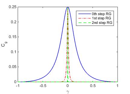
Figure 3: (Color online) Geometric average of the concurrences is plotted against anisotropic parameter $\gamma$ after each step of the RG.

The critical behavior of the entanglement can be seen as a diverging of its derivative when it crosses the phase transition point. The absolute values of the first derivative of the concurrence with respect to $\gamma$ after each iteration are shown in FIG. 4. The diverging behavior of the derivative at $\gamma=0$ can be seen with increasing the RG iterations. While concurrence itself remains continuous. It reveals that the system exhibits the second-order QPT. It is also noted that the entanglement in the vicinity of the critical point shows scaling behavior vedral intro(2) . At the critical point, the entanglement scales logarithmically and saturates away from the critical point xxz24 . As we have discussed earlier a large system $N=5^{n+1},$ can be effectively represented by five sites box with renormalized coupling constants after the $n$th RG iteration. Therefore, the entanglement between the two renormalized sites describes the entanglement between two blocks, each containing $N/5$ sites. We note that the system shows the scaling behavior which is linear when $\ln$ of maximum of the absolute value of first derivative $\ln(\mid dC_{g}/d\gamma\mid_{\max})$ is plotted against $\ln N=\ln 5^{n+1},$ where $n=1,2,3...$. The scaling behavior is shown in FIG. 5. The position of the maximum of $dC_{g}/d\gamma$ approaches the critical point as the size of the system increases. To get more insight, we plot $\ln(\gamma_{c}-\gamma_{\max})$ against $\ln N$ in FIG. 6 and obtain the relation $\gamma_{\max}=\gamma_{c}-(0.33N)^{-\theta},$ where the entanglement exponent $\theta=1.14.$ The entanglement exponent $\theta$ obtained from the RG method captures the behavior of the XY model in the vicinity of the critical point and defined as inverse of the correlation length exponent. In thermodynamic limit, the correlation length covers the entire system as we approach the critical point.

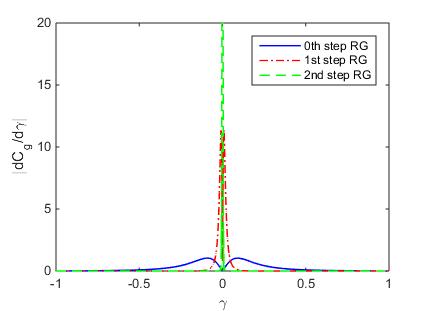
Figure 4: (Color online) Absolute derivative of the geometric average of the concurrences is plotted against $\gamma$ as the RG iteration is increased.

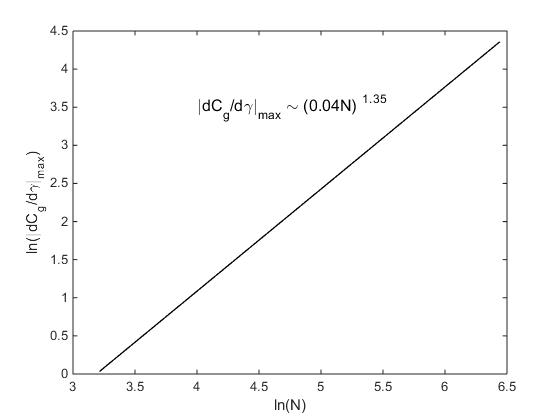
Figure 5: Logarithm of the absolute value of the maximum of the derivative of the concurrence is plotted against the logarithm of N, the system size.

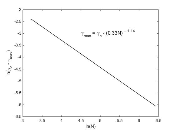
Figure 6: Scaling behavior of $\gamma_{\max}$ is plotted against N the size of the system, where $\gamma_{\max}$ is the position of the maximum of the derivative of the concurrence (see FIG. 6).

IV CONCLUSIONS

Study of the correlated systems in two dimensions through the renormalization group (RG) technique was presented in this paper. For this purpose, square lattice of Heisenberg spin-1/2 XY model was considered. The quantum correlations were explored through concurrence and were related to the quantum phase transition (QPT). Due to the presence of several interblock interactions, we computed geometric average of the concurrences of the all possible interactions between the blocks. We noted that the system size increases rapidly and reaches at the critical point in the less number of the RG iterations as compared to the one-dimensional case which were studied previously xxz ; xxzdm ; xy ; xydm . Moreover, we found that the results for concurrence in 2D are similar to the one-dimensional case qualitatively. But the magnitude of the concurrence is smaller in 2D, because the shared neighbor sites are larger in number in 2D as compared with one-dimensional chain. The evolution of the entanglement after the $n$th RG iteration explains that it develops two values, one non zero value at the critical point and approaches to zero otherwise, which correspond to spin-fluid phase and Ising phase respectively. The relation between the critical point, which is maximum value of the absolute derivative of the concurrence and the system size (scaling behavior) was investigated, which showed a linear behavior. Moreover, the scaling behavior was explored through determination of the entanglement exponent which describes how the critical point is acheived as the size of the system increases.

V ACKNOWLEDGMENTS

This work was partly supported by the HIGHER EDUCATION COMMISSION, PAKISTAN under the Indigenous Ph.D. Fellowship Scheme.

VI APPENDIX

The expression for $\gamma$’s are given below;

$$\gamma_{1} = -\frac{(-1+\alpha_{1}+\gamma^{2})\sqrt{(5+\alpha_{1}+5\gamma^{2}}}{4\sqrt{2\alpha_{2}}},$$

$$\gamma_{2} = -\frac{3\sqrt{\frac{\gamma^{4}(5+\alpha_{1}+5\gamma^{2})}{\alpha_{2}}}}{2\sqrt{2}\gamma},$$

$$\gamma_{3} = \frac{(-1+\alpha_{1}+\gamma^{2})}{\sqrt{2\alpha_{2}}},$$

$$\gamma_{4} = \frac{\gamma(5+\alpha_{1}+\gamma^{2})}{2\sqrt{2\alpha_{2}}},$$

$$\gamma_{5} = \frac{3\sqrt{2}\gamma^{2}}{\alpha_{2}},$$

$$\gamma_{6} = \frac{\sqrt{\frac{\gamma^{2}(5+\alpha_{1}+5\gamma^{2})}{1+\alpha_{1}+34\gamma^{2}-\alpha_{1}\gamma^{2}+\gamma^{4}}}(-2-2\alpha_{1}+17\gamma^{2}-3\alpha_{1}\gamma^{2}+3\gamma^{4})}{4(3+2\gamma^{2}+3\gamma^{4})},$$

$$\gamma_{7} = -\frac{\sqrt{\frac{\gamma^{2}(5+\alpha_{1}+5\gamma^{2})}{1+\alpha_{1}+34\gamma^{2}-\alpha_{1}\gamma^{2}+\gamma^{4}}}(1+\alpha_{1}-\gamma^{2}+6\gamma^{4})}{4\gamma(3+2\gamma^{2}+3\gamma^{4})},$$

$$\gamma_{8} = -\frac{3\sqrt{\frac{\gamma^{2}(5+\alpha_{1}+5\gamma^{2})}{1+\alpha_{1}+34\gamma^{2}-\alpha_{1}\gamma^{2}+\gamma^{4}}}(5-\alpha_{1}+5\gamma^{2})}{4(3+2\gamma^{2}+3\gamma^{4})},$$

$$\gamma_{9} = \frac{(1+\alpha_{1}-\gamma^{2})}{4\gamma\sqrt{(34-\alpha_{1}+\frac{1+\alpha_{1}}{\gamma^{2}}+\gamma^{2})}},$$

$$\gamma_{10} = \frac{3}{2\sqrt{(34-\alpha_{1}+\frac{1+\alpha_{1}}{\gamma^{2}}+\gamma^{2})}},$$

where,

$$\alpha_{1} = \sqrt{1+34\gamma^{2}+\gamma^{4}},$$

$$\alpha_{2} = 2-2\alpha_{1}+71\gamma^{2}+17\alpha_{1}\gamma^{2}+104\gamma^{4}+3\alpha_{1}\gamma^{4}+3\gamma^{6}.$$

References

- (1) C. H. Bennett, G. Brassard, C. Crepeau, R. Jozsa, A. Peres, and W. K. Wootters, Phys. Rev. Lett. 70, 1895 (1993).
- (2) M. A. Nielsen and I. L. Chuang, Quantum Computation and Quantum Communication (Cambridge University Press, Cambridge, 2000).
- (3) T. J. Osborne, and M. A. Nielsen, Phys. Rev. A 66, 032110 (2002).
- (4) G. Vidal, J. I. Latorre, E. Rico, and A. Kitaev, Phys. Rev. Lett. 90, 227902 (2003).
- (5) S. Bose, Phys. Rev. Lett. 91, 207901 (2003).
- (6) A. Osterloh, Luigi Amico, G. Falci, and Rosario Fazio, Nature (London) 416, 608 (2002).
- (7) S. Sachdev, Quantum Phase Transitions (Cambridge University Press, Cambridge, 2000).
- (8) J. S. Bell, Physics 1, 195 (1964).
- (9) X. Wang, Phys. Rev. A 66, 044305 (2002).
- (10) L. Zhou, H. S. Song, Y. Q. Guo, and C. Li, Phys. Rev. A 68, 024301 (2003).
- (11) L. Amico, R. Fazio, A. Osterloh, and V. Vedral, Rev. Mod. Phys. 80, 517 (2008).
- (12) M. Kargarian, R. Jafari, and A. Langari, Phys. Rev. A 76, 060304(R) (2007).
- (13) M. Kargarian, R. Jafari, and A. Langari, Phys. Rev. A 77, 032346 (2008).
- (14) M. Kargarian, R. Jafari, and A. Langari, Phys. Rev. A 79, 042319 (2009).
- (15) Fu-Wu Ma, Sheng-Xin Liu, and Xiang-Mu Kong, Phys. Rev. A 83, 062309 (2011).
- (16) Fu-Wu Ma, Sheng-Xin Liu, and Xiang-Mu Kong, Phys. Rev. A 84, 042302 (2011).
- (17) M. Takahashi, Thermodynamics of One-Dimensional Solvable Models (Cambridge University Press, Cambridge, England, 1999).
- (18) E. Barouch, and B. McCoy, Phys. Rev. A 3, 786 (1971).
- (19) Olav F. Syljuasen Physics Letters A 322 (2004) 25-30.
- (20) Olav F. Syljuasen, Phys. Rev. A 68, 060301(R) (2003).
- (21) Roscilde, T., P. Verrucchi, A. Fubini, S. Haas, and V. Tognetti, Phys. Rev. Lett. 94, 147208 (2005).
- (22) A S T Pires, L S Lima and M E Gouvea, J. Phys.: Condens. Matter 20, 015208 (2008).
- (23) L. X. Hayden, T. A. Kaplan, and S. D. Mahanti, Phys. Rev. Lett. 105, 047203 (2010).
- (24) Gu, S., G. Tian, and H. Lin, Phys. Rev. A 71, 052322 (2005).
- (25) Gu, S., G. Tian, and H. Lin, New J. Phys. 8, 61 (2006).
- (26) Song, J., S. Gu, and H. Lin, Phys. Rev. B 74, 155119 (2006).
- (27) S. R. White, Phys. Rev. Lett. 69, 2863 (1992); Phys. Rev. B 48, 10345 (1993).
- (28) T. Xiang, Phys. Rev. B 53, 10445 (1996).
- (29) T. Nishino, J. Phys. Soc. Jpn. 64, 3598 (1995).
- (30) S. R. White and D. J. Scalapino,Phys. Rev. Lett. 80, 1272 (1998).
- (31) R. Jafari and A. Langari, Phys. A 364, 213 (2006).
- (32) R. Jafari and A. Langari, Phys. Rev. B 76, 014412 (2007).
- (33) A. Langari, Phys. Rev. B 69, 100402(R) (2004).
- (34) J. Gonzalez, M. A. Martin-Deigado, G. Sierrra, and A. H. Vozmediano, Quantum Electron Liquids and High-Tc Superconductivity, edited by H. Araki et al., Lecture Notes in Physics Vol. 38 Springer 1995
- (35) E. Lieb, T. Schultz, and D. Mattis, Ann. Phys. (NY) 16, 407 (1961).
- (36) F. Verstraete, J. I. Cirac, J. I. Latorre, E. Rico, and M. M. Wolf, Phys. Rev. Lett. 94, 140601 (2005).
- (37) S. Hill and W. K. Wootters, Phys. Rev. Lett. 78, 5022 (1997), W. K. Wootters, Phys. Rev. Lett. 80, 2245 (1998).
- (38) J. I. Latorre, E. Rico, and G. Vidal, Quantum Inf. Comput. 4, 48 2004 .