Emergent Phase Space Description of Unitary Matrix Model

Arghya Chattopadhyay111arghya@iiserb.ac.in 1, Parikshit Dutta222parikshitdutta@yahoo.co.in 2,3 and Suvankar Dutta333suvankar@iiserb.ac.in 1
1Department of Physics
Indian Institute of Science Education and Research Bhopal
Bhopal 462 066, India
2Department of Physics, Asutosh College
92, Shyamaprasad Mukherjee Road
Kolkata 700 026, India
3School of Physical Sciences
Jawaharlal Nehru University
New Delhi 110067, India
Abstract:

We show that large N𝑁N phases of a 00 dimensional generic unitary matrix model (UMM) can be described in terms of topologies of two dimensional droplets on a plane spanned by eigenvalue and number of boxes in Young diagram. Information about different phases of UMM is encoded in the geometry of droplets. These droplets are similar to phase space distributions of a unitary matrix quantum mechanics (UMQM) ((0+1)01(0+1) dimensional) on constant time slices. We find that for a given UMM, it is possible to construct an effective UMQM such that its phase space distributions match with droplets of UMM on different time slices at large N𝑁N. Therefore, large N𝑁N phase transitions in UMM can be understood in terms of dynamics of an effective UMQM. From the geometry of droplets it is also possible to construct Young diagrams corresponding to U(N)𝑈𝑁U(N) representations and hence different large N𝑁N states of the theory in momentum space. We explicitly consider two examples : single plaquette model with TrU2Trsuperscript𝑈2\text{Tr}U^{2} terms and Chern-Simons theory on S3superscript𝑆3S^{3}. We describe phases of CS theory in terms of eigenvalue distributions of unitary matrices and find dominant Young distributions for them.

1 Introduction and summary

Unitary matrix model (UMM) has a wide range of applicability both in mathematics and physics. Partition functions of different super-symmetric gauge theories, in particular Chern-Simons theory on certain manifolds boil down to UMMs. These models also have applications in a broad class of condensed matter systems.

A UMM is a statistical ensemble of unitary matrices (denoted by U𝑈U), defined by the partition function

𝒵=[𝒟U]exp[S(U)],where, S(U) is action and 𝒟U is Haar measure.𝒵delimited-[]𝒟𝑈𝑆𝑈where, S(U) is action and 𝒟U is Haar measure.\displaystyle\displaystyle{\cal Z}=\int{[\cal{D}}U]\,\exp\left[S(U)\right],\,\,\,\,\text{where, $S(U)$ is action and ${\cal{D}}U$ is Haar measure.} (1.1)

Both 𝒟U𝒟𝑈{\cal D}U and S(U)𝑆𝑈S(U) are invariant under unitary transformations. Since U𝑈U does not depend on any parameter, this partition function defines a 00-dimensional field theory over unitary matrices. Solution of UMMs in large N𝑁N limit (N𝑁N being dimension of matrix) renders a distribution of eigenvalues (EVs) of unitary matrices. EV distribution captures information of different phases of the system and transition between them.

On the other hand, it is well know that eigenvalues of hermitian (or unitary) matrices behave like positions of free fermions [1, 2]. In hermitian matrix quantum mechanics, dynamics of eigenvalues can be thought of N𝑁N non-interacting fermions moving in a potential V(θ)𝑉𝜃V(\theta). At large N𝑁N all the eigenvalues (fermions) occupy the lowest possible energy states (ground state configuration) of the potential upto a fermi level. Different large N𝑁N phases of the system, therefore, can be explained in terms of shapes of fermi surfaces in phase space. All the states below that surface are occupied, like Thomas-Fermi distribution at zero temperature [3].

Phase space description of matrix quantum mechanics seems to be quite natural because explicit time dependence of eigenvalues allows one to define conjugate momenta associated with eigenvalues. Interacting gauge theories (supersymmetric as well as non-supersymmetric) on compact manifolds can be written as a 0-dimensional UMM [4, 5, 6, 7, 8, 9]. Eigenvalues of these unitary matrices do not dependent on time (or any other parameter). Therefore, it would be interesting to ask if one can provide a similar phase space description for different large N𝑁N phases of these theories in terms of droplets of constant densities in two dimensions. In [10], with a bit of surprise, it was observed that for a very restricted class of matrix models, such description is indeed possible. Writing the partition function as a sum over all possible representations of unitary group one can study large N𝑁N behaviour of the modes in terms of most dominant representation which is characterised by a distribution function u(h)𝑢u(h). u(h)𝑢u(h) measures how boxes hh are distributed in a Young diagram. Solving the model at large N𝑁N, [10] found that information of different phases of the theory can be captured in terms of topologies (shapes) of different droplets in two dimensions. This two dimensional plane is spanned by θ𝜃\theta and hh. Eigenvalue and Young tableaux distributions for different phases of the theory can be obtained from a distributions function ω(h,θ)𝜔𝜃\omega(h,\theta) in (h,θ)𝜃(h,\theta) plane with property

ω(h,θ)=1for(h,θ)R=0otherwise.formulae-sequenceformulae-sequence𝜔𝜃1for𝜃𝑅0otherwise.\displaystyle\displaystyle\begin{split}\omega(h,\theta)&=1\quad\text{for}\quad(h,\theta)\in R\\ &=0\quad\text{otherwise.}\end{split} (1.2)

Eigenvalue distribution ρ(θ)𝜌𝜃\rho(\theta) for a given θ𝜃\theta can be obtained from the distribution by integrating over hh

ρ(θ)=12π0ω(h,θ)𝑑h.𝜌𝜃12𝜋superscriptsubscript0𝜔𝜃differential-d\displaystyle\displaystyle\rho(\theta)=\frac{1}{2\pi}\int_{0}^{\infty}\omega(h,\theta)dh. (1.3)

Similarly, for a given hh, integrating over θ𝜃\theta we obtain Young tableaux distribution,

u(h)=12πππω(h,θ)𝑑θ.𝑢12𝜋superscriptsubscript𝜋𝜋𝜔𝜃differential-d𝜃\displaystyle\displaystyle u(h)=\frac{1}{2\pi}\int_{-\pi}^{\pi}\omega(h,\theta)d\theta\ . (1.4)

The droplet picture of large N𝑁N matrix model is very interesting, as these droplets are similar to those of Thomas-Fermi model where Wigner distribution is assumed to take constant value inside some region in phase space and zero elsewhere. If eigenvalues of unitary matrices are like positions of fermions with distribution function ρ(θ)𝜌𝜃\rho(\theta), then from droplet picture it seems that hh plays the role of momentum with distribution u(h)𝑢u(h). Therefore, we see that droplet picture raises a very intriguing question if there is any underlying quantum mechanics (quantum mechanics of N𝑁N free fermions) associated with different large N𝑁N phases of UMMs (or interacting gauge theories).

Before answering this question, we first need to understand if phase space description is a universal characteristic of UMM. In other words, if all large N𝑁N phases of any UMM can be described in terms of topologies of droplets. An important relation between character of conjugacy class and number of boxes in a Young diagram is required to understand this question. For a class of model considered in [10, 11], the relation is known and simple (character is equal to dimension of representation). However, in general this relation is nontrivial and there exists no exact formula for character444We shall discuss about Frobenius formula in section 3 and see that it offers an expression for character in terms of auxiliary variables.. Therefore, it is difficult to construct u(h)𝑢u(h) directly from partition function. However, in [12], a more general class of matrix model was considered, namely plaquette model and shown that even if it is difficult to find u(h)𝑢u(h) directly from partition function, but a distribution function ω(h,θ)𝜔𝜃\omega(h,\theta) in (h,θ)𝜃(h,\theta) plane can be obtained in large N𝑁N limit. Our first goal, in this paper, is to establish this result for a generic UMM and show that different large N𝑁N phases of a generic unitary matrix model also have an emergent “phase space” description. Our generic model includes multi-trace terms in action. Therefore, this generic matrix model can describe weakly coupled gauge theories on compact manifold.

Before delving deep, it is worth taking a digression and mention about some important works and literature in mathematics and their relevance with our work. As we have already mentioned, different large N𝑁N phases of gauge theory correspond to different asymptotic behaviour of dominant Young diagrams. Asymptotic growth of Young diagrams is a well known process in mathematics. It originated from the pioneering works by A. Vershik and S. Kerov. Details of some of their related works can be found in [13]. Kerov has studied a Markovian growth process of Young diagrams also known as Plancherel growth process (due to involvement of Plancherel measure), and shown that almost all of Young diagrams become uniformly close to a common universal curve. In the current context the work of [14] is also worth mentioning, who gave the asymptotic behaviour of the characters when the corresponding Young diagram converge to some prescribed shape. The key difference between the study of Kerov and others and our work is that we are interested in large N𝑁N shapes of the Young diagram in presence of a potential. As we change the parameters of the theory the potential changes and hence the asymptotic behaviour of the corresponding Young diagram. This is the reason why we are not getting any universal behaviour of the Young diagrams involved in our case and precisely this non-universal behaviour is the reason we have different shapes of the droplets which in turn helps one to differentiate between large N𝑁N phases of the matrix model involved.

Coming back to the main context, in order to understand the underlying quantum mechanics associated with large N𝑁N phases of UMMs, in this paper we observe that droplet picture in (h,θ)𝜃(h,\theta) plane is similar to phase space distribution of a unitary matrix quantum mechanics (UMQM) on a constant time slice. Partition function of UMQM is equivalent to a theory of free fermions [1, 2]. Time evolution of this system can be written as time evolution of two different branches of fermi surface [3]. These different branches of fermi surface define a closed region in phase space. At large N𝑁N all the states inside that region are filled, otherwise empty. There is a relation between eigenvalue (position of fermions) and corresponding momentum which defines the boundary of the region [3]. We see that droplets of UMM have similar feature as phase space distribution of an effective UMQM on a constant time slice. Hamiltonians of both the systems match on that constant time slice. Therefore, given a UMM one can find an underlying matrix quantum mechanics such that its evolution with time from t=ti𝑡subscript𝑡𝑖t=t_{i} to t=tf𝑡subscript𝑡𝑓t=t_{f} captures two different phases of UMM on initial and final time slices. This allows us to understand large N𝑁N phase transition in UMM in terms of dynamics of an effective UMQM. Considering parameters of UMQM to be time dependent one can find a time evolution in effective UMQM such that distributions on initial and final time slices correspond to two different phases of UMM [15]. The idea here is similar to the work of Matytsin [16], who showed that leading term in a non-trivial large-N limit of the Itzykson-Zuber integral can be written in terms of an action functional corresponding to the complex inviscid Burgers (Hopf) equation with boundary conditions specifying the eigenvalue distribution on two different time slices 555[17] extended this study on QCD2 and associated the Douglas-Kazakov phase transition on a cylinder with the presence of gap in the eigenvalue distributions for Wilson loops.. In fact, the time evolution of the action functional is given by a Hamilton-Jacobi form with Hamiltonian similar to collective field theory Hamiltonian of [18, 19]. As we observe in this paper that for a one dimensional unitary matrix model or equivalently an unitary matrix quantum mechanics one ends up with 4.19, which can be re-written as the Hopf equation. Solution of this Hopf equation determines the evolution of asymptotic shape of Young diagram as the system evolves from one phase to other phase in the large N𝑁N limit. Thus evolution of shape of Young diagrams could be related to time evolution of underlying matrix quantum mechanics.

Above result also shows that parameter hh (number of boxes in Young diagram) does indeed play the role of canonical conjugate of eigenvalue θ𝜃\theta. Hence, u(h)𝑢u(h) captures information about momentum distribution for free fermions in effective UMQM in the form of geometry of Young diagram. To explore this further we need to construct Young tableaux distribution u(h)𝑢u(h) from droplet, since finding u(h)𝑢u(h) directly from partition function is difficult for a generic UMM. In this paper we show how one can consistently reconstruct different representations which dominate partition function at large N𝑁N from phase space distribution. We explicitly study two examples to demonstrate the procedure: β1β2subscript𝛽1subscript𝛽2\beta_{1}-\beta_{2} model and Chern-Simons theory on S3superscript𝑆3S^{3}.

Organisation of our paper is following.

  • We start with a very brief introduction of UMM in section 2.

  • In section 3 we discuss emergent phase space description of a generic UMM.

  • Relation between UMM and UMQM has been studied in section 4.

  • We provide an explicit example of reconstruction of Young diagrams from phase space for β1subscript𝛽1\beta_{1}-β2subscript𝛽2\beta_{2} model in section 5.

  • In section 6 we discuss phase space distribution for Chern-Simons theory on S3superscript𝑆3S^{3}. Here we present a unitary matrix model analysis of large N𝑁N phase of CS theory. Then we obtain Young distribution for different values of ’t Hooft coupling.

  • We end our paper with some discussion and out look in section 7.

2 Unitary Matrix Model

2.1 Unitary matrix model and eigenvalue distributions at large N𝑁N

A UMM is a statistical ensemble of unitary matrices, defined by the partition function

𝒵𝒵\displaystyle\displaystyle{\cal Z} =\displaystyle= [𝒟U]exp[S(U)]delimited-[]𝒟𝑈𝑆𝑈\displaystyle\int{[\cal{D}}U]\,\exp\left[S(U)\right] (2.1)

where S(U)𝑆𝑈S(U) is action and 𝒟U𝒟𝑈{\cal{D}}U is Haar measure. Both action and Haar measure are invariant under unitary transformation, hence the partition function. Therefore, one can go to a diagonal basis where U𝑈U is given by

U={eiθi},fori[1,N],θi’s are eigenvalues of U.formulae-sequence𝑈superscript𝑒𝑖subscript𝜃𝑖for𝑖1𝑁θi’s are eigenvalues of U.U=\{e^{i\theta_{i}}\},\quad\text{for}\quad i\in[1,N],\quad\text{$\theta_{i}$'s are eigenvalues of $U$.} (2.2)

In this basis Haar measure takes the following form

[𝒟U]=i=1Nππ𝑑θii<jsin2(θiθj2)delimited-[]𝒟𝑈superscriptsubscriptproduct𝑖1𝑁superscriptsubscript𝜋𝜋differential-dsubscript𝜃𝑖subscriptproduct𝑖𝑗superscript2subscript𝜃𝑖subscript𝜃𝑗2\displaystyle\int[\mathcal{D}U]=\prod_{i=1}^{N}\int_{-\pi}^{\pi}d\theta_{i}\prod_{i<j}\sin^{2}\left(\frac{\theta_{i}-\theta_{j}}{2}\right) (2.3)

and action S(U)𝑆𝑈S(U) becomes function of N𝑁N variables θ1,,θNsubscript𝜃1subscript𝜃𝑁\theta_{1},\cdots,\theta_{N} : V({θi})𝑉subscript𝜃𝑖V(\{\theta_{i}\}). The partition function in this basis is given by

𝒵=i=1Ndθiexp[Seff({θi})]𝒵superscriptsubscriptproduct𝑖1𝑁𝑑subscript𝜃𝑖subscript𝑆effsubscript𝜃𝑖\displaystyle\displaystyle\mathcal{Z}=\int\prod_{i=1}^{N}d\theta_{i}\exp\left[-S_{\text{eff}}({\{\theta_{i}\}})\right] (2.4)

where,

Seff({θi})=V({θi})i=1j<iNln[sin2(θiθj2)].subscript𝑆effsubscript𝜃𝑖𝑉subscript𝜃𝑖superscriptsubscriptFRACOP𝑖1𝑗𝑖𝑁superscript2subscript𝜃𝑖subscript𝜃𝑗2S_{\text{eff}}({\{\theta_{i}\}})=V(\{\theta_{i}\})-\sum_{{i=1}\atop{j<i}}^{N}\ln\left[\sin^{2}\left(\frac{\theta_{i}-\theta_{j}}{2}\right)\right]. (2.5)

The partition function can be thought of as describing a system of N𝑁N particles interacting by a repulsive potential (Coulomb repulsion) ln|sin(θiθj)/2|subscript𝜃𝑖subscript𝜃𝑗2-\ln|\sin(\theta_{i}-\theta_{j})/2| and moving in a common potential V({θi})𝑉subscript𝜃𝑖V(\{\theta_{i}\}). Because of the strong repulsion, two particles (eigenvalues) do not come close to each other. If we neglected the Coulomb repulsion, all eigenvalues would have sat at the minima of potential V(θ)𝑉𝜃V(\theta). But, due to the Coulomb repulsion they spread around these minima and fill some finite intervals.

In large N𝑁N limit one defines a set of continuous variables

θ(x)=θi,wherex=iN[0,1]formulae-sequence𝜃𝑥subscript𝜃𝑖where𝑥𝑖𝑁01\theta(x)={\theta_{i}},\quad\text{where}\quad x={i\over N}\in[0,1] (2.6)

and in terms of these continuous variables the effective action becomes,

Seff({θi})=N2[S[θ(x)]01𝑑x01𝑑ylnsin2(θ(x)θ(y)2)].subscript𝑆effsubscript𝜃𝑖superscript𝑁2delimited-[]𝑆delimited-[]𝜃𝑥superscriptsubscript01differential-d𝑥superscriptsubscript01differential-d𝑦superscript2𝜃𝑥𝜃𝑦2S_{\text{eff}}({\{\theta_{i}\}})=-N^{2}\left[S[\theta(x)]-\int_{0}^{1}dx\mathchoice{{\vbox{\hbox{$\textstyle-$ }}\kern-7.83337pt}}{{\vbox{\hbox{$\scriptstyle-$ }}\kern-5.90005pt}}{{\vbox{\hbox{$\scriptscriptstyle-$ }}\kern-4.75003pt}}{{\vbox{\hbox{$\scriptscriptstyle-$ }}\kern-4.25003pt}}\!\int_{0}^{1}dy\ln\sin^{2}\left({\theta(x)-\theta(y)\over 2}\right)\right]. (2.7)

At large N𝑁N, dominant contribution comes from the saddle points of Seff([θ(x)])subscript𝑆effdelimited-[]𝜃𝑥S_{\text{eff}}({[\theta(x)]}). We define eigenvalue distribution function

ρ(θ)=1Ni=1Nδ(θθi)=|xθ|𝜌𝜃1𝑁superscriptsubscript𝑖1𝑁𝛿𝜃subscript𝜃𝑖𝑥𝜃\displaystyle\displaystyle\begin{split}\rho(\theta)&=\frac{1}{N}\sum_{i=1}^{N}\delta(\theta-\theta_{i})\\ &=\left|{\partial x\over\partial\theta}\right|\end{split} (2.8)

which captures information about distributions of eigenvalues between π𝜋-\pi and π𝜋\pi in large N𝑁N limit. Different saddle points correspond to different eigenvalue distributions and hence different phases of the theory.

2.2 Gauge theory at zero coupling

Thermal partition function of gauge theory on compact manifold (S3superscript𝑆3S^{3}) can be written as a UMM. In zero ’t Hooft coupling limit (λ=gYM2N0𝜆superscriptsubscript𝑔𝑌𝑀2𝑁0\lambda=g_{YM}^{2}N\rightarrow 0), all the modes of the theory are massive with mass terms depending on the size of S3superscript𝑆3S^{3}. Only the zero mode of temporal component of gauge field is massless and strongly interacting. Therefore, in zero coupling limit one can integrate out all the massive modes and obtains an exact partition function in terms of the zero mode. For example, thermal partition function of a SU(N)𝑆𝑈𝑁SU(N) gauge theory on S3×S1superscript𝑆3superscript𝑆1S^{3}\times S^{1} at zero ’t Hooft coupling can be written as,

𝒵(β)=[𝒟U]exp[n=1an(β)nTrUnTrUn]𝒵𝛽delimited-[]𝒟𝑈superscriptsubscript𝑛1subscript𝑎𝑛𝛽𝑛Trsuperscript𝑈𝑛Trsuperscript𝑈absent𝑛\displaystyle\displaystyle\mathcal{Z}(\beta)=\int[\mathcal{D}U]\exp\left[\sum_{n=1}^{\infty}{a_{n}(\beta)\over n}\text{Tr}U^{n}\text{Tr}U^{\dagger n}\right] (2.9)

where U=eiβα𝑈superscript𝑒𝑖𝛽𝛼U=e^{i\beta\alpha}, α𝛼\alpha being zero mode of temporal component of the gauge field and β𝛽\beta (radius of S1superscript𝑆1S^{1}) is inverse temperature. an(β)subscript𝑎𝑛𝛽a_{n}(\beta)’s are related to single particle partition function of bosonic and fermionic modes. See [5, 6, 7, 9] for details.

2.3 Gauge theory at weak coupling

The above equation is derived at zero ’t Hooft coupling. One considers only one loop contribution while integrating out massive modes. In weak ’t Hooft coupling limit one can integrate out massive modes order by order in loop expansion and obtains the following partition function in terms of the holonomy U𝑈U,

𝒵(β,λ)=[𝒟U]exp[Seff(U)]Seff(U)=nan(β)Nki=1kTrUni,withini=0.\displaystyle\displaystyle\begin{split}\mathcal{Z}(\beta,\lambda)&=\int[\mathcal{D}U]\exp[S_{\text{eff}}({U})]\\ S_{\text{eff}}({U})&=\sum_{\vec{n}}{a_{\vec{n}}(\beta)\over N^{k}}\prod_{i=1}^{k}\text{Tr}U^{n_{i}},\quad\text{with}\quad\sum_{i}n_{i}=0.\end{split} (2.10)

Terms, in Seff(U)subscript𝑆eff𝑈S_{\text{eff}}({U}), with k𝑘k traces appears in (k1)𝑘1(k-1) loops in perturbation theory and have a planner contribution starting with λk2superscript𝜆𝑘2\lambda^{k-2}. For example, two trace terms (2.9) comes in one loop order in perturbation theory. In this paper, we show that different large N𝑁N phases of this model has an emergent phase space picture.

2.4 Single plaquette model

A single plaquette model is given by

𝒵(β)=𝒟Uexp[Nn=1βn(β)n(Tr[Un]+Tr[Un])]𝒵𝛽𝒟𝑈𝑁superscriptsubscript𝑛1subscript𝛽𝑛𝛽𝑛Trdelimited-[]superscript𝑈𝑛Trdelimited-[]superscript𝑈absent𝑛\mathcal{Z}(\beta)=\int{\cal{D}}U\,\exp\left[N\sum_{n=1}^{\infty}\frac{\beta_{n}(\beta)}{n}(\text{Tr}[U^{n}]+\text{Tr}[U^{\dagger n}])\right] (2.11)

where βn(β)subscript𝛽𝑛𝛽\beta_{n}(\beta)’s are parameters. This partition function is equivalent to 2.9 with βn(β)subscript𝛽𝑛𝛽\beta_{n}(\beta) identified as an(β)TrUnsubscript𝑎𝑛𝛽delimited-⟨⟩Trsuperscript𝑈𝑛a_{n}(\beta)\left\langle\text{Tr}U^{n}\right\rangle in the large N𝑁N limit. They have similar phase structure.

The single plaquette model has lot of applications in lattice gauge theory. Also, as we shall see, Cherns-Simons theory on S3superscript𝑆3S^{3} can also be written as single plaquette model with βnsubscript𝛽𝑛\beta_{n}’s, determined in terms of ’t Hooft coupling. Single plaquette model has a rich phase structure. We refer to [20, 21] for a detailed study.

3 Emergent phase space distribution

It was first observed in [10] that there exists a relation between eigenvalue density and Young tableaux distribution for a restricted class of matrix models. It was also shown that using these relations, different large N𝑁N phases of the theory can be described in terms of shapes of droplets in two dimensional plane spanned by eigenvalue and number of boxes in Young diagram. However, observation in that paper was accidental and valid for a very limited class of UMM. Also, it was not clear if such identification follows from any extremization condition at large N𝑁N. In [12], work of [10] was generalized to single plaquette model. Most interestingly, [12] showed that the relation between Young distribution and eigenvalue distribution follows from an extremization condition. In this paper we further extend this work to a most generic matrix model of the form (2.10). Although, we work here only upto three trace terms, our construction can be generalised to any arbitrary number of traces.

3.1 Two dimensional droplets for plaquette model

We start our discussion with a brief review of [12]. This discussion will help us to follow the derivation for the most generic case.

Partition function of single plaquette model (2.11) is given by,

𝒵=[𝒟U]exp[Nn=1βnn(TrUn+TrUn)],βn’s are some arbitrary coefficients.𝒵delimited-[]𝒟𝑈𝑁superscriptsubscript𝑛1subscript𝛽𝑛𝑛Trsuperscript𝑈𝑛Trsuperscript𝑈absent𝑛βn’s are some arbitrary coefficients.\mathcal{Z}=\int[\mathcal{D}U]\exp\left[N\sum_{n=1}^{\infty}{\beta_{n}\over n}(\text{Tr}U^{n}+\text{Tr}U^{\dagger n})\right],\quad\text{$\beta_{n}$'s are some arbitrary coefficients.} (3.1)

To obtain phase space distribution, we expand the exponential and write partition function as a sum over representations R𝑅R of unitary group U(N)𝑈𝑁U(N),

𝒵=Rkε(β,k)zklε(β,l)zlχR(C(k))χR(C(l)).𝒵subscript𝑅subscript𝑘𝜀𝛽𝑘subscript𝑧𝑘subscript𝑙𝜀𝛽𝑙subscript𝑧𝑙subscript𝜒𝑅𝐶𝑘subscript𝜒𝑅𝐶𝑙\displaystyle\displaystyle\mathcal{Z}=\sum_{R}\sum_{\vec{k}}\frac{\varepsilon(\vec{\beta},\vec{k})}{z_{\vec{k}}}\sum_{\vec{l}}\frac{\varepsilon(\vec{\beta},\vec{l})}{z_{\vec{l}}}\chi_{R}(C(\vec{k}))\chi_{R}(C(\vec{l})). (3.2)

Here χR(C(k))subscript𝜒𝑅𝐶𝑘\chi_{R}(C(\vec{k})) is the character of conjugacy class C(k)𝐶𝑘C(\vec{k}) of permutation group SKsubscript𝑆𝐾S_{K}, K=nnkn𝐾subscript𝑛𝑛subscript𝑘𝑛K=\sum_{n}nk_{n} and

ε(β,k)=n=1Nknβnkn,zk=n=1kn!nkn.formulae-sequence𝜀𝛽𝑘superscriptsubscriptproduct𝑛1superscript𝑁subscript𝑘𝑛superscriptsubscript𝛽𝑛subscript𝑘𝑛subscript𝑧𝑘superscriptsubscriptproduct𝑛1subscript𝑘𝑛superscript𝑛subscript𝑘𝑛\displaystyle\displaystyle\varepsilon(\vec{\beta},\vec{k})=\prod_{n=1}^{\infty}N^{k_{n}}\beta_{n}^{k_{n}},\quad z_{\vec{k}}=\prod_{n=1}^{\infty}k_{n}!n^{k_{n}}. (3.3)

To derive equation (3.2) we have used the following identity

n(TrUn)kn=RχR(C(k))TrR[U]subscriptproduct𝑛superscriptTrsuperscript𝑈𝑛subscript𝑘𝑛subscript𝑅subscript𝜒𝑅𝐶𝑘subscriptTr𝑅delimited-[]𝑈\prod_{n}(\text{Tr}U^{n})^{k_{n}}=\sum_{R}\chi_{R}(C(\vec{k}))\text{Tr}_{R}[U] (3.4)

and the normalisation condition666See [22, 23, 24] for details.

𝒟UTrR[U]TrR[U]=δRR.𝒟𝑈subscriptTr𝑅delimited-[]𝑈subscriptTrsuperscript𝑅delimited-[]superscript𝑈subscript𝛿𝑅superscript𝑅\int{\cal{D}}U\,\text{Tr}_{R}[U]\text{Tr}_{R^{\prime}}[U^{\dagger}]=\delta_{RR^{\prime}}. (3.5)

Sum of representation of U(N)𝑈𝑁U(N) can be written as a sum over different Young diagrams. If K𝐾K is the total number of boxes in a Young diagram with λisubscript𝜆𝑖\lambda_{i} being the number of boxes in i𝑖i-th row then i=1Nλi=Ksuperscriptsubscript𝑖1𝑁subscript𝜆𝑖𝐾\sum_{i=1}^{N}\lambda_{i}=K. Hence, sum over representations can be decomposed as

RK=1{λi}δ(i=1NλiK)withλ1λ2λN0.formulae-sequencesubscript𝑅superscriptsubscript𝐾1subscriptsubscript𝜆𝑖𝛿superscriptsubscript𝑖1𝑁subscript𝜆𝑖𝐾withsubscript𝜆1subscript𝜆2subscript𝜆𝑁0\sum_{R}\longrightarrow\sum_{K=1}^{\infty}\,\sum_{\{\lambda_{i}\}}\ \delta\left(\sum_{i=1}^{N}\lambda_{i}-K\right)\quad\text{with}\quad\lambda_{1}\geq\lambda_{2}\geq\cdots\geq\lambda_{N}\geq 0. (3.6)

The partition function, therefore, can be written as,

𝒵=λk,lε(β,k)ε(β,l)zkzlχλ(C(k))χλ(C(l))δ(nnkniλi)δ(nnlniλi).𝒵subscript𝜆subscript𝑘𝑙𝜀𝛽𝑘𝜀𝛽𝑙subscript𝑧𝑘subscript𝑧𝑙subscript𝜒𝜆𝐶𝑘subscript𝜒𝜆𝐶𝑙𝛿subscript𝑛𝑛subscript𝑘𝑛subscript𝑖subscript𝜆𝑖𝛿subscript𝑛𝑛subscript𝑙𝑛subscript𝑖subscript𝜆𝑖\displaystyle\displaystyle\mathcal{Z}=\sum_{\vec{\lambda}}\sum_{\vec{k},\vec{l}}\frac{\varepsilon(\vec{\beta},\vec{k})\varepsilon(\vec{\beta},\vec{l})}{z_{\vec{k}}z_{\vec{l}}}\chi_{\vec{\lambda}}(C(\vec{k}))\chi_{\vec{\lambda}}(C(\vec{l}))\ \delta\left(\sum_{n}nk_{n}-\sum_{i}\lambda_{i}\right)\delta\left(\sum_{n}nl_{n}-\sum_{i}\lambda_{i}\right). (3.7)

We introduce N𝑁N variables h1,,hNsubscript1subscript𝑁h_{1},\cdots,h_{N}, related to number of boxes λisubscript𝜆𝑖\lambda_{i}’s as

hi=λi+Nii=1,,N.formulae-sequencesubscript𝑖subscript𝜆𝑖𝑁𝑖for-all𝑖1𝑁\displaystyle h_{i}=\lambda_{i}+N-i\qquad\forall\quad i=1,\cdots,N. (3.8)

hisubscript𝑖h_{i}’s are shifted number of boxes777Our terminology is little sloppy. We also call hisubscript𝑖h_{i} as the number of boxes in the i𝑖i-th row.. From monotonicity of λisubscript𝜆𝑖\lambda_{i}s it follows that hisubscript𝑖h_{i}s satisfy the following constraint

h1>h2>>hN0.subscript1subscript2subscript𝑁0h_{1}>h_{2}>\cdots>h_{N}\geq 0. (3.9)

From now on we shall use variables hisubscript𝑖h_{i}s in stead of λisubscript𝜆𝑖\lambda_{i}s.

In large N𝑁N limit we define continuous variables

hiN=h(x),kn=N2kn,x=iNwithx[0,1].formulae-sequencesubscript𝑖𝑁𝑥formulae-sequencesubscript𝑘𝑛superscript𝑁2subscriptsuperscript𝑘𝑛formulae-sequence𝑥𝑖𝑁with𝑥01\displaystyle{h_{i}\over N}=h(x),\quad\quad k_{n}=N^{2}k^{\prime}_{n},\quad\quad x={i\over N}\quad\text{with}\quad x\in[0,1]. (3.10)

In this limit summation over i𝑖i is replaced by an integral over x𝑥x,

α=1N01𝑑xsuperscriptsubscript𝛼1𝑁superscriptsubscript01differential-d𝑥\sum_{\alpha=1}^{\infty}\rightarrow N\int_{0}^{1}dx (3.11)

and sum over representations (λ𝜆\vec{\lambda}) and sum over cycles (knsubscript𝑘𝑛k_{n}) are given by path integral over h(x)𝑥h(x) and integral over knsuperscriptsubscript𝑘𝑛k_{n}^{\prime}. Writing characters χhsubscript𝜒\chi_{\vec{h}} in terms of h(x)𝑥h(x) and knsuperscriptsubscript𝑘𝑛k_{n}^{\prime}, partition function (3.7), in large N𝑁N limit, can be written as

𝒵=[𝒟h(x)]n𝑑kn𝑑lnexp[N2Seff[h(x),kn,ln]],𝒵delimited-[]𝒟𝑥subscriptproduct𝑛differential-dsuperscriptsubscript𝑘𝑛differential-dsuperscriptsubscript𝑙𝑛superscript𝑁2subscript𝑆eff𝑥superscriptsubscript𝑘𝑛superscriptsubscript𝑙𝑛\mathcal{Z}=\int[\mathcal{D}h(x)]\prod_{n}\int dk_{n}^{\prime}dl_{n}^{\prime}\exp\left[-N^{2}S_{\text{eff}}[h(x),\vec{k_{n}^{\prime}},\vec{l_{n}^{\prime}}]\right], (3.12)

where Seffsubscript𝑆effS_{\text{eff}} is the effective action. Dominant contribution to partition function comes from those representations which maximise effective action Seffsubscript𝑆effS_{\text{eff}}. To find the most dominant representations at large N𝑁N, we introduce a function called Young tableaux density defined as,

u(h)=xh.𝑢𝑥u(h)=-{\partial x\over\partial h}. (3.13)

Different Young diagrams correspond to different u(h)𝑢u(h). Since h(x)𝑥h(x) is a monotonically decreasing function of x𝑥x, Young density has an upper and lower cap 1u(h)0x[0,1]1𝑢0for-all𝑥011\geq u(h)\geq 0\ \forall\ x\in[0,1].

For the simplest case, β10subscript𝛽10\beta_{1}\neq 0 and other βn=0subscript𝛽𝑛0\beta_{n}=0 (for n2𝑛2n\geq 2) one can find u(h)𝑢u(h) for different phases of the model [10, 11]. In this simple case we need to calculate character of permutation group in presence of one cycles only (kn=0subscript𝑘𝑛0k_{n}=0 for n2𝑛2n\geq 2) which is given by dimension of the corresponding representation. As a result is was possible for [10, 11] to extremize the effective action to obtain u(h)𝑢u(h) for different phases888A large N𝑁N phase transition corresponds to a qualitative change in nature of this dominant representation as one varies the parameters. The Douglas-Kazakov phase transition [25, 26] and its generalisations in 2d Yang-Mills theory can be understood this way.. [10, 11] also observed that there exists a beautiful identification between Young tableaux distribution and eigenvalue distribution for all the phases of the theory,

h±=12+β1cosθ±πρ(θ),andu(h)=θπformulae-sequencesubscriptplus-or-minusplus-or-minus12subscript𝛽1𝜃𝜋𝜌𝜃and𝑢𝜃𝜋\displaystyle\displaystyle h_{\pm}=\frac{1}{2}+\beta_{1}\cos\theta\pm\pi\rho(\theta),\quad\text{and}\quad u(h)={\theta\over\pi} (3.14)

where h±subscriptplus-or-minush_{\pm} are solutions of the following equation

h2(1+2β1cosθ)h+14(1+2β1cosθ)2=π2ρ2(θ).superscript212subscript𝛽1𝜃14superscript12subscript𝛽1𝜃2superscript𝜋2superscript𝜌2𝜃h^{2}-(1+2\beta_{1}\cos\theta)h+\frac{1}{4}(1+2\beta_{1}\cos\theta)^{2}=\pi^{2}\rho^{2}(\theta). (3.15)

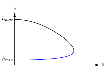
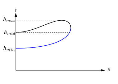
This identification allows one to write eigenvalue distribution and Young tableaux distribution in terms of a single constant distribution function ω(h,θ)𝜔𝜃\omega(h,\theta) given by equations (1.3) and (1.4). h±(θ)subscriptplus-or-minus𝜃h_{\pm}(\theta) defines the boundary of the distribution. It is actually the shape (or boundary) of the region R𝑅R which contains all the information about two distributions for a given phase of the model. Thus, a relation between hh and θ𝜃\theta defines disjoint islands (phase space distribution/droplet) in two dimensions for different phases of the UMM under consideration. Different phases are distinguished by different topologies of droplets. Constant phase space distribution is very similar to Thomas-Fermi (TF) model [27, 28] at zero temperature.

The identification, observed in [10, 11], between two distribution was accidental. It was not known if such identification holds for a generic model like (3.1). The main obstacle to apply the idea of [10] to a generic UMM was finding character in terms of hisubscript𝑖h_{i}s in presence of arbitrary cycles. Presence of TrUnTrsuperscript𝑈𝑛\text{Tr}U^{n} term in partition function requires to calculate character in presence of n𝑛n-cycles. Hence, finding u(h)𝑢u(h) by extremizing the effective action for a generic unitary matrix model was a challenging problem.

In [12] it was shown that, although it is difficult to find u(h)𝑢u(h) for a generic plaquette model (3.1), but one can still find droplets for different phases of the theory and from the shape of these droplets one can reconstruct dominant Young diagram.

3.1.1 Frobenius formula for character

Let C(k)𝐶𝑘C({\vec{k}}) denotes the conjugacy class of SKsubscript𝑆𝐾S_{K} which is determined by a collection of sequence of numbers

k=(k1,k2,),with,nnkn=K.formulae-sequence𝑘subscript𝑘1subscript𝑘2withsubscript𝑛𝑛subscript𝑘𝑛𝐾\displaystyle\vec{k}=(k_{1},k_{2},\cdots),\qquad\text{with},\ \ \sum_{n}nk_{n}=K. (3.16)

C(k)𝐶𝑘C({\vec{k}}) consists of permutations having k1subscript𝑘1k_{1} number of 1-cycles, k2subscript𝑘2k_{2} number of 2-cycles and so on. We introduce a set of independent variables, x1,,xNsubscript𝑥1subscript𝑥𝑁x_{1},\cdots,x_{N}. The character corresponding to a conjugacy class C(k)𝐶𝑘C(\vec{k}) of SKsubscript𝑆𝐾S_{K} for a representation characterized by λ𝜆\vec{\lambda} is given by famous Frobenius formula

χh(Ck)=[Δ(x).n(Pn(x))kn](h1,,hN)\displaystyle\chi_{\vec{h}}(C_{\vec{k}})=\bigg{[}\Delta(x).\prod_{n}\left(P_{n}(x)\right)^{k_{n}}\bigg{]}_{(h_{1},\cdots,h_{N})} (3.17)

where

Pn(x)=i=1Nxin,Δ(x)=i<j(xixj)formulae-sequencesubscript𝑃𝑛𝑥superscriptsubscript𝑖1𝑁superscriptsubscript𝑥𝑖𝑛Δ𝑥subscriptproduct𝑖𝑗subscript𝑥𝑖subscript𝑥𝑗\displaystyle P_{n}(x)=\sum_{i=1}^{N}x_{i}^{n},\quad\quad\Delta(x)=\prod_{i<j}(x_{i}-x_{j}) (3.18)

and hisubscript𝑖h_{i}’s are give by equation (3.8). The notation [](h1,,hN)subscriptdelimited-[]subscript1subscript𝑁[\cdots]_{(h_{1},\cdots,h_{N})} implies

[f(x)](h1,,hN)=coefficient of x1h1xNhN in f(x).subscriptdelimited-[]𝑓𝑥subscript1subscript𝑁coefficient of superscriptsubscript𝑥1subscript1superscriptsubscript𝑥𝑁subscript𝑁 in 𝑓𝑥\left[f(x)\right]_{(h_{1},\cdots,h_{N})}=\textrm{coefficient of }x_{1}^{h_{1}}\cdots x_{N}^{h_{N}}\textrm{ in }f(x). (3.19)

3.1.2 Extremization of partition function

Promoting N𝑁N real variables x1,,xNsubscript𝑥1subscript𝑥𝑁x_{1},\cdots,x_{N} in (3.17) to N𝑁N complex variable (z1,z2,zN)subscript𝑧1subscript𝑧2subscript𝑧𝑁(z_{1},z_{2},\cdots z_{N}) character can be written as,

χh(Ck)=α=1N12πidzαzαhα+1[(α=1Nzα)k1(α=1Nzα2)k2α<β(zαzβ)].subscript𝜒subscript𝐶𝑘superscriptsubscriptproduct𝛼1𝑁contour-integral12𝜋𝑖𝑑subscript𝑧𝛼superscriptsubscript𝑧𝛼subscript𝛼1delimited-[]superscriptsuperscriptsubscript𝛼1𝑁subscript𝑧𝛼subscript𝑘1superscriptsuperscriptsubscript𝛼1𝑁superscriptsubscript𝑧𝛼2subscript𝑘2subscriptproduct𝛼𝛽subscript𝑧𝛼subscript𝑧𝛽\displaystyle\chi_{\vec{h}}(C_{\vec{k}})=\prod_{\alpha=1}^{N}\oint\frac{1}{2\pi i}\frac{dz_{\alpha}}{z_{\alpha}^{h_{\alpha}+1}}\left[\left(\sum_{\alpha=1}^{N}z_{\alpha}\right)^{k_{1}}\left(\sum_{\alpha=1}^{N}z_{\alpha}^{2}\right)^{k_{2}}\cdots\prod_{\alpha<\beta}(z_{\alpha}-z_{\beta})\right]. (3.20)

The contour is taken around origin. Note that, in the above expressions for character (equation 3.17 or 3.20) variables xisubscript𝑥𝑖x_{i}’s or zisubscript𝑧𝑖z_{i}’s are auxiliary variables. They do not carry any physical meaning, as of now.

Integrand in the above expression can be exponentiated and written as,

χh(Ck)=α=1N12πidzαzαexp[n=1knln(α=1Nzαn)+12αβln|zαzβ|α=1Nhαlnza].subscript𝜒subscript𝐶𝑘superscriptsubscriptproduct𝛼1𝑁contour-integral12𝜋𝑖𝑑subscript𝑧𝛼subscript𝑧𝛼superscriptsubscript𝑛1subscript𝑘𝑛superscriptsubscript𝛼1𝑁superscriptsubscript𝑧𝛼𝑛12subscript𝛼𝛽subscript𝑧𝛼subscript𝑧𝛽superscriptsubscript𝛼1𝑁subscript𝛼subscript𝑧𝑎\displaystyle\chi_{\vec{h}}(C_{\vec{k}})=\prod_{\alpha=1}^{N}\oint\frac{1}{2\pi i}\frac{dz_{\alpha}}{z_{\alpha}}\exp\left[\sum_{n=1}^{\infty}k_{n}\ln(\sum_{\alpha=1}^{N}z_{\alpha}^{n})+\frac{1}{2}\sum_{\alpha\neq\beta}\ln|z_{\alpha}-z_{\beta}|-\sum_{\alpha=1}^{N}h_{\alpha}\ln z_{a}\right]. (3.21)

Therefore, in large N𝑁N limit character is given by,

χ[h(x),C(k)]=(12πi)N[𝒟z(x)]z(x)exp[N2Sχ(h[x],k)]𝜒𝑥𝐶superscript𝑘superscript12𝜋𝑖𝑁contour-integraldelimited-[]𝒟𝑧𝑥𝑧𝑥superscript𝑁2subscript𝑆𝜒delimited-[]𝑥superscript𝑘\displaystyle\displaystyle\chi[h(x),C(\vec{k^{\prime}})]=\left(\frac{1}{2\pi i}\right)^{N}\oint{[\mathcal{D}z(x)]\over z(x)}\exp[-N^{2}S_{\chi}(h[x],\vec{k^{\prime}})] (3.22)

where action Sχsubscript𝑆𝜒S_{\chi} is given by

Sχ(h[x],k)subscript𝑆𝜒delimited-[]𝑥superscript𝑘\displaystyle\displaystyle-S_{\chi}(h[x],\vec{k^{\prime}}) =\displaystyle= n=1kn[(n+1)lnN+ln(01𝑑xzn(x))]+1201𝑑x01𝑑yln|z(x)z(y)|superscriptsubscript𝑛1superscriptsubscript𝑘𝑛delimited-[]𝑛1𝑁superscriptsubscript01differential-d𝑥superscript𝑧𝑛𝑥12superscriptsubscript01differential-d𝑥superscriptsubscript01differential-d𝑦𝑧𝑥𝑧𝑦\displaystyle\sum_{n=1}^{\infty}k_{n}^{\prime}\left[(n+1)\ln N+\ln\left(\int_{0}^{1}dxz^{n}(x)\right)\right]+\frac{1}{2}\int_{0}^{1}dx\mathchoice{{\vbox{\hbox{$\textstyle-$ }}\kern-7.83337pt}}{{\vbox{\hbox{$\scriptstyle-$ }}\kern-5.90005pt}}{{\vbox{\hbox{$\scriptscriptstyle-$ }}\kern-4.75003pt}}{{\vbox{\hbox{$\scriptscriptstyle-$ }}\kern-4.25003pt}}\!\int_{0}^{1}dy\ln|z(x)-z(y)| (3.23)
KlnN01𝑑xh(x)lnz(x)superscript𝐾𝑁superscriptsubscript01differential-d𝑥𝑥𝑧𝑥\displaystyle\quad-K^{\prime}\ln N-\int_{0}^{1}dxh(x)\ln z(x)

and N2K=K=total number of boxes in a representationsuperscript𝑁2superscript𝐾𝐾total number of boxes in a representationN^{2}K^{\prime}=K=\text{total number of boxes in a representation}.

Using the expression for character given in equation (3.22), partition function (3.7) can be written as,

𝒵=𝒩n𝑑kn𝑑ln𝒟h(x)𝒟z(x)𝒟w(x)𝑑t𝑑sexp(N2Stotal[h,z,w,k,l,t,s])𝒵𝒩subscriptproduct𝑛differential-dsuperscriptsubscript𝑘𝑛differential-dsuperscriptsubscript𝑙𝑛𝒟𝑥contour-integral𝒟𝑧𝑥contour-integral𝒟𝑤𝑥superscriptsubscriptdifferential-d𝑡superscriptsubscriptdifferential-d𝑠superscript𝑁2subscript𝑆total𝑧𝑤superscript𝑘superscript𝑙𝑡𝑠\displaystyle\displaystyle\mathcal{Z}=\mathcal{N}\prod_{n}\int dk_{n}^{\prime}dl_{n}^{\prime}\int\mathcal{D}h(x)\oint\mathcal{D}z(x)\oint{\cal{D}}w(x)\int_{-\infty}^{\infty}dt\int_{-\infty}^{\infty}ds\exp\left(-N^{2}S_{\text{total}}\left[h,z,w,\vec{k^{\prime}},\vec{l^{\prime}},t,s\right]\right)

where,

Stotal[h,z,w,k,l,t,s]=n[kn(1+ln(βnZnnkn))+ln(1+ln(βnWnnln))]+1201𝑑x01𝑑y(ln|z(x)z(y)|+ln|w(x)w(y)|)01𝑑xh(x)lnz(x)w(x)+it(nnknK)+is(nnlnK).subscript𝑆total𝑧𝑤superscript𝑘superscript𝑙𝑡𝑠subscript𝑛delimited-[]superscriptsubscript𝑘𝑛1subscript𝛽𝑛subscript𝑍𝑛𝑛superscriptsubscript𝑘𝑛superscriptsubscript𝑙𝑛1subscript𝛽𝑛subscript𝑊𝑛𝑛superscriptsubscript𝑙𝑛12superscriptsubscript01differential-d𝑥superscriptsubscript01differential-d𝑦𝑧𝑥𝑧𝑦𝑤𝑥𝑤𝑦superscriptsubscript01differential-d𝑥𝑥𝑧𝑥𝑤𝑥𝑖𝑡subscript𝑛𝑛superscriptsubscript𝑘𝑛superscript𝐾𝑖𝑠subscript𝑛𝑛superscriptsubscript𝑙𝑛superscript𝐾\displaystyle\begin{split}-S_{\text{total}}\left[h,z,w,\vec{k^{\prime}},\vec{l^{\prime}},t,s\right]&=\sum_{n}\bigg{[}k_{n}^{\prime}\left(1+\ln\left({\beta_{n}Z_{n}\over nk_{n}^{\prime}}\right)\right)+l_{n}^{\prime}\left(1+\ln\left({\beta_{n}W_{n}\over nl_{n}^{\prime}}\right)\right)\bigg{]}\\ &\qquad+\frac{1}{2}\int_{0}^{1}dx\mathchoice{{\vbox{\hbox{$\textstyle-$ }}\kern-7.83337pt}}{{\vbox{\hbox{$\scriptstyle-$ }}\kern-5.90005pt}}{{\vbox{\hbox{$\scriptscriptstyle-$ }}\kern-4.75003pt}}{{\vbox{\hbox{$\scriptscriptstyle-$ }}\kern-4.25003pt}}\!\int_{0}^{1}dy\left(\ln|z(x)-z(y)|+\ln|w(x)-w(y)|\right)\\ &\qquad-\int_{0}^{1}dxh(x)\ln z(x)w(x)+it\left(\sum_{n}nk_{n}^{\prime}-K^{\prime}\right)+is\left(\sum_{n}nl_{n}^{\prime}-K^{\prime}\right).\end{split} (3.25)

Varying effective action with respect to z(x)𝑧𝑥z(x) we find999Similar equation can be obtained when we vary action with respect to w(x)𝑤𝑥w(x).,

nnknZnzn(x)+01dyz(x)z(x)z(y)h(x)=0\displaystyle\displaystyle\sum_{n}{nk_{n}^{\prime}\over Z_{n}}z^{n}(x)+\mathchoice{{\vbox{\hbox{$\textstyle-$ }}\kern-7.83337pt}}{{\vbox{\hbox{$\scriptstyle-$ }}\kern-5.90005pt}}{{\vbox{\hbox{$\scriptscriptstyle-$ }}\kern-4.75003pt}}{{\vbox{\hbox{$\scriptscriptstyle-$ }}\kern-4.25003pt}}\!\int_{0}^{1}dy{z(x)\over z(x)-z(y)}-h(x)=0 (3.26)

where,

Zn=01𝑑xzn(x).subscript𝑍𝑛superscriptsubscript01differential-d𝑥superscript𝑧𝑛𝑥Z_{n}=\int_{0}^{1}dxz^{n}(x). (3.27)

Varying effective action with respect to h(x)𝑥h(x) we find,

z(x)w(x)=ei(t+s)=constant (independent ofx).z(x)w(x)=e^{-i(t+s)}=\text{constant (independent of}\ x). (3.28)

Variation with respect to knsuperscriptsubscript𝑘𝑛k_{n}^{\prime} and lnsuperscriptsubscript𝑙𝑛l_{n}^{\prime} provides,

βnZnnkn=eitn,andβnWnnln=eisn.formulae-sequencesubscript𝛽𝑛subscript𝑍𝑛𝑛superscriptsubscript𝑘𝑛superscript𝑒𝑖𝑡𝑛andsubscript𝛽𝑛subscript𝑊𝑛𝑛superscriptsubscript𝑙𝑛superscript𝑒𝑖𝑠𝑛\displaystyle\displaystyle{\beta_{n}Z_{n}\over nk_{n}^{\prime}}=e^{-itn},\quad\text{and}\quad{\beta_{n}W_{n}\over nl_{n}^{\prime}}=e^{-isn}. (3.29)

Since, in equation (3.1.2) z(x)𝑧𝑥z(x) and w(x)𝑤𝑥w(x) vary over some contour around zero, we take these contours to be unit circle about the origin and hence a consistent solution to above equations are,

z(x)=eiθ(x),w(x)=eiθ(x),andt=s=0.formulae-sequence𝑧𝑥superscript𝑒𝑖𝜃𝑥formulae-sequence𝑤𝑥superscript𝑒𝑖𝜃𝑥and𝑡𝑠0z(x)=e^{i\theta(x)},\quad w(x)=e^{-i\theta(x)},\quad\text{and}\quad t=s=0. (3.30)

Therefore,

kn=ln=βnρnn,whereZn=𝑑θρ(θ)cosnθρn.formulae-sequencesuperscriptsubscript𝑘𝑛superscriptsubscript𝑙𝑛subscript𝛽𝑛subscript𝜌𝑛𝑛wheresubscript𝑍𝑛differential-d𝜃𝜌𝜃𝑛𝜃subscript𝜌𝑛k_{n}^{\prime}=l_{n}^{\prime}={\beta_{n}\rho_{n}\over n},\quad\text{where}\quad Z_{n}=\int d\theta\rho(\theta)\cos n\theta\equiv\rho_{n}. (3.31)

Thus saddle point equation (3.26) becomes,

nnknZneinθ+ππ𝑑θρ(θ)eiθeiθeiθh(θ)=0,whereρ(θ)=xθ.formulae-sequencesubscript𝑛𝑛superscriptsubscript𝑘𝑛subscript𝑍𝑛superscript𝑒𝑖𝑛𝜃superscriptsubscript𝜋𝜋differential-dsuperscript𝜃𝜌superscript𝜃superscript𝑒𝑖𝜃superscript𝑒𝑖𝜃superscript𝑒𝑖superscript𝜃𝜃0where𝜌𝜃𝑥𝜃\sum_{n}{nk_{n}^{\prime}\over Z_{n}}e^{in\theta}+\mathchoice{{\vbox{\hbox{$\textstyle-$ }}\kern-7.83337pt}}{{\vbox{\hbox{$\scriptstyle-$ }}\kern-5.90005pt}}{{\vbox{\hbox{$\scriptscriptstyle-$ }}\kern-4.75003pt}}{{\vbox{\hbox{$\scriptscriptstyle-$ }}\kern-4.25003pt}}\!\int_{-\pi}^{\pi}d\theta^{\prime}\rho(\theta^{\prime})\frac{e^{i\theta}}{e^{i\theta}-e^{i\theta^{\prime}}}-h(\theta)=0,\quad\text{where}\quad\rho(\theta)={\partial x\over\partial\theta}. (3.32)

Evaluating the partition function (3.1.2) on these equations we find,

𝒵=𝒩[𝒟θ]exp[N2n=12βnnρn+N212𝑑θρ(θ)𝑑θρ(θ)ln|4sin2(θθ2)|].𝒵𝒩delimited-[]𝒟𝜃superscript𝑁2superscriptsubscript𝑛12subscript𝛽𝑛𝑛subscript𝜌𝑛superscript𝑁212differential-d𝜃𝜌𝜃differential-dsuperscript𝜃𝜌superscript𝜃4superscript2𝜃superscript𝜃2\displaystyle\begin{split}\mathcal{Z}&=\mathcal{N}\int[\mathcal{D}\theta]\exp\left[N^{2}\sum_{n=1}^{\infty}2\frac{\beta_{n}}{n}\rho_{n}+N^{2}\frac{1}{2}\mathchoice{{\vbox{\hbox{$\textstyle-$ }}\kern-7.83337pt}}{{\vbox{\hbox{$\scriptstyle-$ }}\kern-5.90005pt}}{{\vbox{\hbox{$\scriptscriptstyle-$ }}\kern-4.75003pt}}{{\vbox{\hbox{$\scriptscriptstyle-$ }}\kern-4.25003pt}}\!\int d\theta\rho(\theta)\mathchoice{{\vbox{\hbox{$\textstyle-$ }}\kern-7.83337pt}}{{\vbox{\hbox{$\scriptstyle-$ }}\kern-5.90005pt}}{{\vbox{\hbox{$\scriptscriptstyle-$ }}\kern-4.75003pt}}{{\vbox{\hbox{$\scriptscriptstyle-$ }}\kern-4.25003pt}}\!\int d\theta^{\prime}\rho(\theta^{\prime})\ln\left|4\sin^{2}\left(\frac{\theta-\theta^{\prime}}{2}\right)\right|\right].\end{split} (3.33)

This partition function is exactly same as the partition function of one plaquette model written as an integral over eigenvalues of unitary matrices. Hence, we identify that the auxiliary variables we used to write the character of symmetric group with eigenvalues of corresponding unitary matrix model involved. Imaginary part of saddle point equation (3.32) becomes equation for eigenvalue density,

nnknZnsinnθ12ππ𝑑θρ(θ)cot(θθ2)=0.subscript𝑛𝑛superscriptsubscript𝑘𝑛subscript𝑍𝑛𝑛𝜃12superscriptsubscript𝜋𝜋differential-dsuperscript𝜃𝜌superscript𝜃𝜃superscript𝜃20\displaystyle\displaystyle\sum_{n}{nk_{n}^{\prime}\over Z_{n}}\sin{n\theta}-\frac{1}{2}\mathchoice{{\vbox{\hbox{$\textstyle-$ }}\kern-7.83337pt}}{{\vbox{\hbox{$\scriptstyle-$ }}\kern-5.90005pt}}{{\vbox{\hbox{$\scriptscriptstyle-$ }}\kern-4.75003pt}}{{\vbox{\hbox{$\scriptscriptstyle-$ }}\kern-4.25003pt}}\!\int_{-\pi}^{\pi}d\theta^{\prime}\rho(\theta^{\prime})\cot\left({\theta-\theta^{\prime}\over 2}\right)=0. (3.34)

On the other hand, the real part of equation (3.32) provides a relation between hh and θ𝜃\theta,

h(θ)=12+nnknZncosnθ.𝜃12subscript𝑛𝑛superscriptsubscript𝑘𝑛subscript𝑍𝑛𝑛𝜃h(\theta)=\frac{1}{2}+\sum_{n}{nk_{n}^{\prime}\over Z_{n}}\cos{n\theta}. (3.35)

However, this equation is not complete. It is easy to check that total action (3.25) is invariant under

h(θ)h(θ)+f(θ)𝜃𝜃𝑓𝜃h(\theta)\rightarrow h(\theta)+f(\theta) (3.36)

where, f(θ)𝑓𝜃f(\theta) is an even function of θ𝜃\theta. Hence, the most generic form of h(θ)𝜃h(\theta) is given by,

h(θ)=12+nnknZncosnθ+f(θ).𝜃12subscript𝑛𝑛superscriptsubscript𝑘𝑛subscript𝑍𝑛𝑛𝜃𝑓𝜃h(\theta)=\frac{1}{2}+\sum_{n}{nk_{n}^{\prime}\over Z_{n}}\cos{n\theta}+f(\theta). (3.37)

Form of f(θ)𝑓𝜃f(\theta) can be fixed from topological structure of droplets for different phases [12] and is given by f(θ)=πρ(θ)𝑓𝜃𝜋𝜌𝜃f(\theta)=\pi\rho(\theta). Finally we have,

h±(θ)=S(θ)±πρ(θ),S(θ)=12+nβncosnθ.formulae-sequencesubscriptplus-or-minus𝜃plus-or-minus𝑆𝜃𝜋𝜌𝜃𝑆𝜃12subscript𝑛subscript𝛽𝑛𝑛𝜃h_{\pm}(\theta)=S(\theta)\pm\pi\rho(\theta),\quad S(\theta)=\frac{1}{2}+\sum_{n}{\beta_{n}}\cos{n\theta}. (3.38)

This equation defines the shape of constant droplets in (h,θ)𝜃(h,\theta) plane. This equation is generalization of the relation given in equation (3.14). Thus we see that for a generalised plaquette model all the phases of the theory can be characterised in terms of topologies of different droplets in two dimensional plane spanned by hh and θ𝜃\theta.

3.2 Two dimensional droplets for generic unitary matrix model

We start with an action which contains maximum three traces,

Seff=n1,n2all valuesan1n2N3TrUn1TrUn2TrU(n1+n2).subscript𝑆𝑒𝑓𝑓subscriptFRACOPsubscript𝑛1subscript𝑛2all valuessubscript𝑎subscript𝑛1subscript𝑛2superscript𝑁3Trsuperscript𝑈subscript𝑛1Trsuperscript𝑈subscript𝑛2Trsuperscript𝑈absentsubscript𝑛1subscript𝑛2\displaystyle S_{eff}=\sum_{{n_{1},n_{2}\atop\text{all values}}}{a_{n_{1}n_{2}}\over N^{3}}\text{Tr}{U^{n_{1}}}\text{Tr}{U^{n_{2}}}\text{Tr}{U^{\dagger(n_{1}+n_{2})}}. (3.39)

When n1subscript𝑛1n_{1} (or n2subscript𝑛2n_{2}) is zero we get back one loop (zero coupling) action. The above action is invariant under UU𝑈superscript𝑈U\rightarrow U^{\dagger} if an1n2=an1n2subscript𝑎subscript𝑛1subscript𝑛2subscript𝑎subscript𝑛1subscript𝑛2a_{n_{1}n_{2}}=a_{-n_{1}-n_{2}}, and can also be written as,

Seff=n1,n20an1n2N3(TrUn1TrUn2TrU(n1+n2)+TrUn1TrUn2TrU(n1+n2))subscript𝑆𝑒𝑓𝑓subscriptsubscript𝑛1subscript𝑛20subscript𝑎subscript𝑛1subscript𝑛2superscript𝑁3Trsuperscript𝑈subscript𝑛1Trsuperscript𝑈subscript𝑛2Trsuperscript𝑈absentsubscript𝑛1subscript𝑛2Trsuperscript𝑈absentsubscript𝑛1Trsuperscript𝑈absentsubscript𝑛2Trsuperscript𝑈subscript𝑛1subscript𝑛2\displaystyle S_{eff}=\sum_{n_{1},n_{2}\geq 0}{a_{n_{1}n_{2}}\over N^{3}}\Bigg{(}\text{Tr}{U^{n_{1}}}\text{Tr}{U^{n_{2}}}\text{Tr}{U^{\dagger(n_{1}+n_{2})}}+\text{Tr}{U^{\dagger n_{1}}}\text{Tr}{U^{\dagger n_{2}}}\text{Tr}{U^{(n_{1}+n_{2})}}\Bigg{)} (3.40)

which is manifestly invariant under UU𝑈superscript𝑈U\rightarrow U^{\dagger{}}.

Following the same analysis as discussed in previous section we find a saddle point equation for auxiliary variables appearing in the Frobenius formula as (see appendix A for details),

n1n2=0(n1kn1n2Zn1ein1θ+n2kn1n2Zn2ein2θ+(n1+n2)kn1n2Zn1+n2ei(n1+n2)θ)superscriptsubscriptsubscript𝑛1subscript𝑛20subscript𝑛1superscriptsubscript𝑘subscript𝑛1subscript𝑛2subscript𝑍subscript𝑛1superscript𝑒𝑖subscript𝑛1𝜃subscript𝑛2superscriptsubscript𝑘subscript𝑛1subscript𝑛2subscript𝑍subscript𝑛2superscript𝑒𝑖subscript𝑛2𝜃subscript𝑛1subscript𝑛2superscriptsubscript𝑘subscript𝑛1subscript𝑛2subscript𝑍subscript𝑛1subscript𝑛2superscript𝑒𝑖subscript𝑛1subscript𝑛2𝜃\displaystyle\displaystyle\sum_{n_{1}n_{2}=0}^{\infty}\left({n_{1}k_{n_{1}n_{2}}^{\prime}\over Z_{n_{1}}}e^{in_{1}\theta}+{n_{2}k_{n_{1}n_{2}}^{\prime}\over Z_{n_{2}}}e^{in_{2}\theta}+{(n_{1}+n_{2})k_{n_{1}n_{2}}^{\prime}\over Z_{n_{1}+n_{2}}}e^{i(n_{1}+n_{2})\theta}\right)
i2𝑑θρ(θ)cot(θθ2)+12h(θ)𝑖2differential-dsuperscript𝜃𝜌superscript𝜃𝜃superscript𝜃212𝜃\displaystyle-{i\over 2}\ \mathchoice{{\vbox{\hbox{$\textstyle-$ }}\kern-7.83337pt}}{{\vbox{\hbox{$\scriptstyle-$ }}\kern-5.90005pt}}{{\vbox{\hbox{$\scriptscriptstyle-$ }}\kern-4.75003pt}}{{\vbox{\hbox{$\scriptscriptstyle-$ }}\kern-4.25003pt}}\!\int d\theta^{\prime}\,\rho(\theta^{\prime})\cot\left({\theta-\theta^{\prime}\over 2}\right)+\frac{1}{2}-h(\theta) =\displaystyle= 00\displaystyle 0 (3.41)

where, ρ(θ)𝜌𝜃\rho(\theta) is defined in equation (3.32). Imaginary part of this equation gives eigenvalue equation

n1n2=0[n1kn1n2Zn1sin(n1θ)+n2kn1n2Zn2sin(n2θ)+(n1+n2)ln1n2Zn1+n2sin((n1+n2)θ)]superscriptsubscriptsubscript𝑛1subscript𝑛20delimited-[]subscript𝑛1superscriptsubscript𝑘subscript𝑛1subscript𝑛2subscript𝑍subscript𝑛1subscript𝑛1𝜃subscript𝑛2superscriptsubscript𝑘subscript𝑛1subscript𝑛2subscript𝑍subscript𝑛2subscript𝑛2𝜃subscript𝑛1subscript𝑛2superscriptsubscript𝑙subscript𝑛1subscript𝑛2subscript𝑍subscript𝑛1subscript𝑛2subscript𝑛1subscript𝑛2𝜃\displaystyle\sum_{n_{1}n_{2}=0}^{\infty}\left[{n_{1}k_{n_{1}n_{2}}^{\prime}\over Z_{n_{1}}}\sin(n_{1}\theta)+{n_{2}k_{n_{1}n_{2}}^{\prime}\over Z_{n_{2}}}\sin(n_{2}\theta)+{(n_{1}+n_{2})l_{n_{1}n_{2}}^{\prime}\over Z_{n_{1}+n_{2}}}\sin\left((n_{1}+n_{2})\theta\right)\right]\ \
1201𝑑θρ(θ)cot(θθ2)12superscriptsubscript01differential-dsuperscript𝜃𝜌superscript𝜃𝜃superscript𝜃2\displaystyle-{1\over 2}\ \mathchoice{{\vbox{\hbox{$\textstyle-$ }}\kern-7.83337pt}}{{\vbox{\hbox{$\scriptstyle-$ }}\kern-5.90005pt}}{{\vbox{\hbox{$\scriptscriptstyle-$ }}\kern-4.75003pt}}{{\vbox{\hbox{$\scriptscriptstyle-$ }}\kern-4.25003pt}}\!\int_{0}^{1}d\theta^{\prime}\,\rho(\theta^{\prime})\cot\left({\theta-\theta^{\prime}\over 2}\right) =\displaystyle= 0.0\displaystyle 0.\ \ \ \ \ \ (3.42)

Integrating over h(x)𝑥h(x), the partition function can be written as

𝒵=N4(2πi)2N𝒵superscript𝑁4superscript2𝜋𝑖2𝑁\displaystyle\mathcal{Z}={N^{4}\over(2\pi i)^{2N}}\int [Dθ]exp[n1,n2=02N2an1n2ρn1ρn2ρn1+n2\displaystyle[D\theta]\exp\Bigg{[}\sum_{n_{1},n_{2}=0}^{\infty}2N^{2}a_{n_{1}n_{2}}^{\prime}\rho_{n_{1}}\rho_{n_{2}}\rho_{n_{1}+n_{2}} (3.43)
+N22dθρ(θ)dθρ(θ)(ln 4sin2(θθ2)+ln 4)].\displaystyle+\frac{N^{2}}{2}\int d\theta\rho(\theta)\mathchoice{{\vbox{\hbox{$\textstyle-$ }}\kern-7.83337pt}}{{\vbox{\hbox{$\scriptstyle-$ }}\kern-5.90005pt}}{{\vbox{\hbox{$\scriptscriptstyle-$ }}\kern-4.75003pt}}{{\vbox{\hbox{$\scriptscriptstyle-$ }}\kern-4.25003pt}}\!\int d\theta^{\prime}\rho(\theta^{\prime})\left(\ln\,4\sin^{2}\left(\frac{\theta-\theta^{\prime}}{2}\right)+\ln\,4\right)\Bigg{]}.

Thus we see, even for a general matrix model auxiliary variables in Frobenius formula are same as eigenvalues of unitary matrices.

The real part of saddle point equation defines the shape of constant droplets in (h,θ)𝜃(h,\theta) plane

h±(θ)=S(θ)±πρ(θ).subscriptplus-or-minus𝜃plus-or-minus𝑆𝜃𝜋𝜌𝜃\displaystyle h_{\pm}(\theta)=S(\theta)\pm\pi\rho(\theta). (3.44)

where,

S(θ)=12+n1n2=0an1n2ρn1ρn2ρn1+n2(n1cosn1θρn1+n2cosn2θρn2+(n1+n2)cos(n1+n2)θρn1ρn2).𝑆𝜃12superscriptsubscriptsubscript𝑛1subscript𝑛20subscriptsuperscript𝑎subscript𝑛1subscript𝑛2subscript𝜌subscript𝑛1subscript𝜌subscript𝑛2subscript𝜌subscript𝑛1subscript𝑛2subscript𝑛1subscript𝑛1𝜃subscript𝜌subscript𝑛1subscript𝑛2subscript𝑛2𝜃subscript𝜌subscript𝑛2subscript𝑛1subscript𝑛2subscript𝑛1subscript𝑛2𝜃subscript𝜌subscript𝑛1subscript𝜌subscript𝑛2S(\theta)={1\over 2}+\sum_{n_{1}n_{2}=0}^{\infty}a^{\prime}_{n_{1}n_{2}}\rho_{n_{1}}\rho_{n_{2}}\rho_{n_{1}+n_{2}}\Bigg{(}{n_{1}\cos n_{1}\theta\over\rho_{n_{1}}}+{n_{2}\cos n_{2}\theta\over\rho_{n_{2}}}+{(n_{1}+n_{2})\cos(n_{1}+n_{2})\theta\over\rho_{n_{1}}\rho_{n_{2}}}\Bigg{)}. (3.45)

This is a generalization of equation (3.38). It is easy to check that all the expressions matches with those of plaquette model for n2=0subscript𝑛20n_{2}=0 with 2n1an10ρn1=βn12subscript𝑛1subscriptsuperscript𝑎subscript𝑛10subscript𝜌subscript𝑛1subscript𝛽subscript𝑛12n_{1}a^{\prime}_{n_{1}0}\rho_{n_{1}}=\beta_{n_{1}}.

Although here we considered three trace terms only, a generalisation to arbitrary model is straightforward. However, algebra will be little difficult.

4 Unitary matrix quantum mechanics and phase space distribution

h±subscriptplus-or-minush_{\pm} in generalized boundary relation (3.38 or 3.44) is a solution of the following quadratic equation

h22S(θ)h+S2(θ)π2ρ2(θ)=0.superscript22𝑆𝜃superscript𝑆2𝜃superscript𝜋2superscript𝜌2𝜃0h^{2}-2S(\theta)h+S^{2}(\theta)-\pi^{2}\rho^{2}(\theta)=0. (4.1)

We define a distribution function ω(h,θ)𝜔𝜃\omega(h,\theta) in (h,θ)𝜃(h,\theta) plane

ω(h,θ)=Θ((hh(θ))(h+(θ)h)2)𝜔𝜃Θsubscript𝜃subscript𝜃2\omega(h,\theta)=\Theta\left({(h-h_{-}(\theta))(h_{+}(\theta)-h)\over 2}\right) (4.2)

such that ω(h,θ)=1𝜔𝜃1\omega(h,\theta)=1 for h(θ)<h<h+(θ)subscript𝜃subscript𝜃h_{-}(\theta)<h<h_{+}(\theta) and zero otherwise. Eigenvalue distribution, by construction, can be obtained by integrating out hh for a given θ𝜃\theta (equation 1.3) and is given by

ρ(θ)=h+(θ)h(θ)2π.𝜌𝜃subscript𝜃subscript𝜃2𝜋\rho(\theta)={h_{+}(\theta)-h_{-}(\theta)\over 2\pi}. (4.3)

Wilson loops are given by

TrUn=12π0𝑑hππ𝑑θcosnθω(h,θ).delimited-⟨⟩Trsuperscript𝑈𝑛12𝜋superscriptsubscript0differential-dsuperscriptsubscript𝜋𝜋differential-d𝜃𝑛𝜃𝜔𝜃\left\langle\text{Tr}U^{n}\right\rangle=\frac{1}{2\pi}\int_{0}^{\infty}dh\int_{-\pi}^{\pi}d\theta\ \cos n\theta\ \omega(h,\theta). (4.4)

The function S(θ)𝑆𝜃S(\theta) can also be written in terms of phase space geometry

S(θ)=12πρ0𝑑hhω(h,θ)=h+(θ)+h(θ)2.𝑆𝜃12𝜋𝜌superscriptsubscript0differential-d𝜔𝜃subscript𝜃subscript𝜃2S(\theta)=\frac{1}{2\pi\rho}\int_{0}^{\infty}dh\ h\ \omega(h,\theta)={h_{+}(\theta)+h_{-}(\theta)\over 2}. (4.5)

The droplet picture of different large N𝑁N phases are similar to droplets of Thomas-Fermi (TF) model at zero temperature. Fermi distribution at zero temperature is given by

Δ(p,q)=Θ(μ𝔥(p,q))Δ𝑝𝑞Θ𝜇𝔥𝑝𝑞\Delta(p,q)=\Theta(\mu-\mathfrak{h}(p,q)) (4.6)

where μ𝜇\mu is chemical potential and 𝔥(p,q)𝔥𝑝𝑞\mathfrak{h}(p,q) is single particle Hamiltonian density. Comparing our phase space distribution (4.2) with TF distribution we find the Hamiltonian density is given by

𝔥(h,θ)=h22S(θ)h+g(θ)2+μ,whereg(θ)=h+(θ)h(θ).formulae-sequence𝔥𝜃superscript22𝑆𝜃𝑔𝜃2𝜇where𝑔𝜃subscript𝜃subscript𝜃\displaystyle\displaystyle\mathfrak{h}(h,\theta)={h^{2}\over 2}-S(\theta)h+{g(\theta)\over 2}+\mu,\quad\text{where}\quad g(\theta)=h_{+}(\theta)h_{-}(\theta). (4.7)

Total Hamiltonian can be obtained by integrating 𝔥(h,θ)𝔥𝜃\mathfrak{h}(h,\theta) over the phase space

Hh=12πππ𝑑θhh+𝑑hω(h,θ)𝔥(h,θ).subscript𝐻12𝜋superscriptsubscript𝜋𝜋differential-d𝜃superscriptsubscriptsubscriptsubscriptdifferential-d𝜔𝜃𝔥𝜃\displaystyle\displaystyle\begin{split}H_{h}&=\frac{1}{2\pi}\int_{-\pi}^{\pi}d\theta\int_{h_{-}}^{h_{+}}dh\ \omega(h,\theta)\ \mathfrak{h}(h,\theta).\end{split} (4.8)

Integrating over hh we find Hamiltonian as a functional of ρ(θ)𝜌𝜃\rho(\theta)

Hh[ρ]=12𝑑θ(π2ρ33S2ρ+gρ)+μ.subscript𝐻delimited-[]𝜌12differential-d𝜃superscript𝜋2superscript𝜌33superscript𝑆2𝜌𝑔𝜌𝜇\displaystyle\displaystyle H_{h}[\rho]=\frac{1}{2}\int d\theta\left({\pi^{2}\rho^{3}\over 3}-S^{2}\rho+g\rho\right)+\mu. (4.9)

This is TF energy functional. As a consistency, one can check that extremization of this Hamiltonian with respect to ρ𝜌\rho gives eigenvalue distribution (4.3).

The Hamiltonian can also be written as

Hh=𝑑θ(S2ρ2+π2ρ36)+Veff(ρ)+μ=12π𝑑h𝑑θ(h22+Veff(θ))ω(h,θ)+μsubscript𝐻differential-d𝜃superscript𝑆2𝜌2superscript𝜋2superscript𝜌36subscript𝑉𝑒𝑓𝑓𝜌𝜇12𝜋differential-ddifferential-d𝜃superscript22subscript𝑉𝑒𝑓𝑓𝜃𝜔𝜃𝜇\begin{split}H_{h}&=\int d\theta\left(\frac{S^{2}\rho}{2}+\frac{\pi^{2}\rho^{3}}{6}\right)+V_{eff}(\rho)+\mu\\ &=\frac{1}{2\pi}\int dh\ d\theta\left(\frac{h^{2}}{2}+V_{eff}(\theta)\right)\omega(h,\theta)\ +\ \mu\end{split} (4.10)

for some Veff(θ)subscript𝑉𝑒𝑓𝑓𝜃V_{eff}(\theta). For example, for simple β1subscript𝛽1\beta_{1} model S(U)=β1(TrU+TrU)𝑆𝑈subscript𝛽1Tr𝑈Trsuperscript𝑈S(U)=\beta_{1}(\text{Tr}U+\text{Tr}U^{\dagger}), Veff(θ)=β1cosθβ12/2cos2θsubscript𝑉𝑒𝑓𝑓𝜃subscript𝛽1𝜃superscriptsubscript𝛽1222𝜃V_{eff}(\theta)=-\beta_{1}\cos\theta-\beta_{1}^{2}/2\cos 2\theta.

4.1 Unitary matrix quantum mechanics

We start with a unitary matrix quantum mechanics

𝒵t=[DU]exp[𝑑t(TrU˙2+W(U))].subscript𝒵𝑡delimited-[]𝐷𝑈differential-d𝑡Trsuperscript˙𝑈2𝑊𝑈\displaystyle\displaystyle\mathcal{Z}_{t}=\int[DU]\exp\left[\int dt\left(\text{Tr}\dot{U}^{2}+W(U)\right)\right]. (4.11)

This matrix model is equivalent to a theory of free fermions on circle with Hamiltonian [1, 2]

HF=𝑑θ(ΨΨ+W(U)ΨΨ)subscript𝐻𝐹differential-d𝜃superscriptΨΨ𝑊𝑈superscriptΨΨH_{F}=\int d\theta\left(\partial\Psi^{\dagger}\partial\Psi+W(U)\Psi^{\dagger}\Psi\right) (4.12)

and with eigenvalue density ΨΨsimilar-toabsentsuperscriptΨΨ\sim\Psi^{\dagger}\Psi. The matrix model (4.11) can also be described as a real bosonic field theory of eigenvalue density ρ(θ,t)𝜌𝜃𝑡\rho(\theta,t) on S1superscript𝑆1S^{1} [19, 29, 18, 15]. Corresponding Hamiltonian is given by,

HB=𝑑θ(12π(t,θ)θρ(t,θ)π(t,θ)θ+π2ρ3(t,θ)6+W(θ)ρ(t,θ))subscript𝐻𝐵differential-d𝜃12𝜋𝑡𝜃𝜃𝜌𝑡𝜃𝜋𝑡𝜃𝜃superscript𝜋2superscript𝜌3𝑡𝜃6𝑊𝜃𝜌𝑡𝜃H_{B}=\int d\theta\left(\frac{1}{2}{\partial\pi(t,\theta)\over\partial\theta}\rho(t,\theta){\partial\pi(t,\theta)\over\partial\theta}+\frac{\pi^{2}\rho^{3}(t,\theta)}{6}+W(\theta)\rho(t,\theta)\right) (4.13)

where, π(θ,t)𝜋𝜃𝑡\pi(\theta,t) is momentum conjugate to ρ(θ,t)𝜌𝜃𝑡\rho(\theta,t). Equations of motion for collective fields are given by,

tρ(t,θ)+θ(ρ(t,θ)v(t,θ))=0tv(t,θ)+12θv(t,θ)2+π22θρ(t,θ)2=W(θ)subscript𝑡𝜌𝑡𝜃subscript𝜃𝜌𝑡𝜃𝑣𝑡𝜃0subscript𝑡𝑣𝑡𝜃12subscript𝜃𝑣superscript𝑡𝜃2superscript𝜋22subscript𝜃𝜌superscript𝑡𝜃2superscript𝑊𝜃\displaystyle\displaystyle\begin{split}\partial_{t}\rho(t,\theta)+\partial_{\theta}\left(\rho(t,\theta)v(t,\theta)\right)&=0\\ \partial_{t}v(t,\theta)+\frac{1}{2}\partial_{\theta}v(t,\theta)^{2}+\frac{\pi^{2}}{2}\partial_{\theta}\rho(t,\theta)^{2}&=-W^{\prime}(\theta)\end{split} (4.14)

where

v(t,θ)=θπ(t,θ).𝑣𝑡𝜃subscript𝜃𝜋𝑡𝜃v(t,\theta)=\partial_{\theta}\pi(t,\theta). (4.15)

These are coupled, non-linear partial differential equation and hence difficult to find a solution in general. Therefore, one can translate the problem into free fermi language [3]. At large N𝑁N, time evolution of the fermionic system can be described in terms of time evolution of fermi surface in phase space. Denoting phase space density by ϖ(p,θ)italic-ϖ𝑝𝜃\varpi(p,\theta) the Hamiltonian is given by,

Hp=12π𝑑θ𝑑p(p22+W(θ))ϖ(p,θ)subscript𝐻𝑝12𝜋differential-d𝜃differential-d𝑝superscript𝑝22𝑊𝜃italic-ϖ𝑝𝜃H_{p}=\frac{1}{2\pi}\int d\theta\ dp\left(\frac{p^{2}}{2}+W(\theta)\right)\varpi(p,\theta) (4.16)

where 𝑑θW(θ)ρ(θ,t)=W(U(t))differential-d𝜃𝑊𝜃𝜌𝜃𝑡𝑊𝑈𝑡\int d\theta W(\theta)\rho(\theta,t)=W(U(t)) and p𝑝p is momentum (conjugate of θ𝜃\theta). This Hamiltonian has the same form as (4.10) except the fact that (p(t),θ(t))𝑝𝑡𝜃𝑡(p(t),\theta(t)) in (4.16) are functions of “t𝑡t”. There is a one to one correspondence between phase space variables and collective field theory variables. Eigenvalue density and corresponding momentum are given by [3]

ρ(θ,t)=12π𝑑pϖ(p,θ),θπ(θ,t)=12πρ𝑑ppϖ(p,θ).formulae-sequence𝜌𝜃𝑡12𝜋differential-d𝑝italic-ϖ𝑝𝜃subscript𝜃𝜋𝜃𝑡12𝜋𝜌differential-d𝑝𝑝italic-ϖ𝑝𝜃\displaystyle\displaystyle\rho(\theta,t)=\frac{1}{2\pi}\int dp\ \varpi(p,\theta),\quad\partial_{\theta}\pi(\theta,t)=\frac{1}{2\pi\rho}\int dp\ p\ \varpi(p,\theta). (4.17)

Assuming p(t,θ)𝑝𝑡𝜃p(t,\theta) ranges from p(t,θ)subscript𝑝𝑡𝜃p_{-}(t,\theta) to p+(t,θ)subscript𝑝𝑡𝜃p_{+}(t,\theta) for a fixed θ𝜃\theta we land up with following dictionary between bosonic and fermionic variables

ρ(t,θ)=p+(t,θ)p(t,θ)2π,andv(t,θ)=p+(t,θ)+p(t,θ)2.formulae-sequence𝜌𝑡𝜃subscript𝑝𝑡𝜃subscript𝑝𝑡𝜃2𝜋and𝑣𝑡𝜃subscript𝑝𝑡𝜃subscript𝑝𝑡𝜃2\rho(t,\theta)={p_{+}(t,\theta)-p_{-}(t,\theta)\over 2\pi},\quad\text{and}\quad v(t,\theta)={p_{+}(t,\theta)+p_{-}(t,\theta)\over 2}. (4.18)

Using this dictionary the Hamiltonian (4.16) reduces to Hamiltonian (4.13). Also, using this dictionary one can show that coupled non-linear differential equations for ρ(t,θ)𝜌𝑡𝜃\rho(t,\theta) and v(t,θ)𝑣𝑡𝜃v(t,\theta) take simpler form in fermionic language

tp±(t,θ)+p±(t,θ)θp±(t,θ)+W(θ)=0.subscript𝑡subscript𝑝plus-or-minus𝑡𝜃subscript𝑝plus-or-minus𝑡𝜃subscript𝜃subscript𝑝plus-or-minus𝑡𝜃superscript𝑊𝜃0\displaystyle\displaystyle\partial_{t}p_{\pm}(t,\theta)+p_{\pm}(t,\theta)\partial_{\theta}p_{\pm}(t,\theta)+W^{\prime}(\theta)=0. (4.19)

These are decoupled first order quasi-linear partial differential equations. p±(t,θ)subscript𝑝plus-or-minus𝑡𝜃p_{\pm}(t,\theta) defines fermi surface in (p,θ)𝑝𝜃(p,\theta) plane. The above equation (4.19) determines evolution of fermi surface with time. Thus solving the field theory equations of motion (4.14) is equivalent to solve for upper and lower fermi surfaces in fermionic picture. In either case, one needs to provide an initial data on a constant time slice in (t,θ)𝑡𝜃(t,\theta) plane. After that the problem reduces to a Cauchy problem. Existence of unique solution depends on the geometry of initial data curve.

Inverting the dictionary (4.18) we find

p±(θ,t)=v(t,θ)±πρ(t,θ).subscript𝑝plus-or-minus𝜃𝑡plus-or-minus𝑣𝑡𝜃𝜋𝜌𝑡𝜃p_{\pm}(\theta,t)=v(t,\theta)\pm\pi\rho(t,\theta). (4.20)

These equations for fermi surface have similarity with generalized boundary relation (3.44) in (h,θ)𝜃(h,\theta) plane. Therefore, on a constant t𝑡t slice101010In finite temperature version, constant time slices are constant temperature slices., one can match fermi surfaces p±(t,θ)subscript𝑝plus-or-minus𝑡𝜃p_{\pm}(t,\theta) with boundary of large N𝑁N droplets (3.44) of a generic UMM (2.1). In other words, large N𝑁N phase space distribution can be used as initial (or terminal) data for the Cauchy problem,

p±(t0,θ)=h±(θ).subscript𝑝plus-or-minussubscript𝑡0𝜃subscriptplus-or-minus𝜃p_{\pm}(t_{0},\theta)=h_{\pm}(\theta). (4.21)

In the bosonic language this is equivalent to v(t0,θ)=S(θ)𝑣subscript𝑡0𝜃𝑆𝜃v(t_{0},\theta)=S(\theta) and ρ(t0,θ)=ρ(θ)𝜌subscript𝑡0𝜃𝜌𝜃\rho(t_{0},\theta)=\rho(\theta). A general phase space distribution (3.44) therefore can be thought of as initial (or terminal) geometry of an underlying quantum mechanics problem. hh which was related to number of boxes in dominant Young representation, is indeed behave like momentum conjugate to θ𝜃\theta. In other words momentum p𝑝p, conjugate to θ𝜃\theta in UMQM has a meaning in terms of boxes in Young diagram. The initial data curve (4.21), we have chosen, is non-characteristic and hence the solution to equation (4.19) is unique.

Thus we see that for any large N𝑁N phase of a generic UMM (2.1) it is possible to construct an effective UMQM such that phase space distribution of matrix quantum mechanics matches with that of UMM on a constant time slice. The effective matrix quantum mechanics has a potential W(θ)=Veff(θ)𝑊𝜃subscript𝑉𝑒𝑓𝑓𝜃W(\theta)=V_{eff}(\theta). The Hamiltonian (4.16) evaluated on t=t0𝑡subscript𝑡0t=t_{0} slice boils down to (4.10)

Hpsubscript𝐻𝑝\displaystyle\displaystyle H_{p}\ tt0Hh𝑡subscript𝑡0absentsubscript𝐻\displaystyle\xrightarrow{t\rightarrow t_{0}}\ H_{h} (4.22)

up to a constant piece.

Unitary matrix model (2.1) shows a rich phase structure at large N𝑁N. The model has many possible phases. As we vary the parameters of the theory the system undergoes a phase transition. It would be interesting to understand the phase transition in UMM in terms of dynamics of effective matrix quantum mechanics. One can allow the parameters of W(θ)𝑊𝜃W(\theta) in UMQM to depend on t𝑡t such that dynamics of UMQM captures phase transition of UMM. We choose UMQM such that on a constant time slices W(θ)𝑊𝜃W(\theta) matches with Veff(θ)subscript𝑉𝑒𝑓𝑓𝜃V_{eff}(\theta) of UMM for different phases.

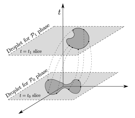
Refer to caption
Figure 1: Time evolution of phases of UMM

As depicted in figure 1 we can start with a particular phase 𝒫0subscript𝒫0\mathcal{P}_{0} of UMM at t=t0𝑡subscript𝑡0t=t_{0} with W(θ(t0),t0)=Veff𝒫0(θ)𝑊𝜃subscript𝑡0subscript𝑡0subscriptsuperscript𝑉subscript𝒫0𝑒𝑓𝑓𝜃W(\theta(t_{0}),t_{0})=V^{\mathcal{P}_{0}}_{eff}(\theta) and use droplet of 𝒫0subscript𝒫0\mathcal{P}_{0} as initial data for the Cauchy problem. Then we let the system evolve with time and some later time t=t1>t0𝑡subscript𝑡1subscript𝑡0t=t_{1}>t_{0} we have W(θ(t1),t1)=Veff𝒫1(θ)𝑊𝜃subscript𝑡1subscript𝑡1subscriptsuperscript𝑉subscript𝒫1𝑒𝑓𝑓𝜃W(\theta(t_{1}),t_{1})=V^{\mathcal{P}_{1}}_{eff}(\theta) and shape of fermi surfaces matches with droplets of 𝒫1subscript𝒫1\mathcal{P}_{1} phase. This will help us in understanding the question how dynamics of strongly interacting gauge theories are encoded in dynamics of free fermions. A work in this direction was considered in [15] for a simpler model111111Look at [30] for a recent paper., where they started with a no-gap distribution at t𝑡t\rightarrow-\infty and showed that time evolution takes this phase to a one-gap phase at t𝑡t\rightarrow\infty. However, for a generic model, we need to thoroughly study the solutions of quasi-linear equations 4.19. We leave the issue for future.

For a unitary matrix quantum mechanics, phase space has θθ𝜃𝜃\theta\rightarrow-\theta symmetry. Using this fact it is possible to show that phase space area covered by fermi surface is a constant of motion. Area covered by fermi surfaces at a time t𝑡t is given by

𝒜(t)=θ0θ0(p+(t,θ)p(t,θ))𝑑θ.𝒜𝑡superscriptsubscriptsubscript𝜃0subscript𝜃0subscript𝑝𝑡𝜃subscript𝑝𝑡𝜃differential-d𝜃\mathcal{A}(t)=\int_{-\theta_{0}}^{\theta_{0}}\left(p_{+}(t,\theta)-p_{-}(t,\theta)\right)d\theta. (4.23)

Using equation (4.19) and the fact that p±(t,θ)subscript𝑝plus-or-minus𝑡𝜃p_{\pm}(t,\theta) and W(θ)𝑊𝜃W(\theta) are symmetric functions of θ𝜃\theta it is easy to verify that

ddt𝒜(t)=0.𝑑𝑑𝑡𝒜𝑡0\frac{d}{dt}\mathcal{A}(t)=0. (4.24)

Thus, phase space area is preserved during time evolution. Its only the shape which changes during evolution.

4.2 Momentum distribution and Young tableaux

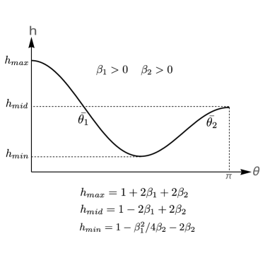
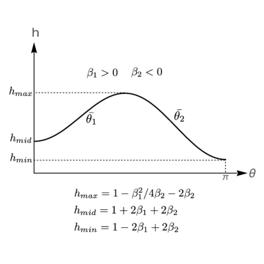
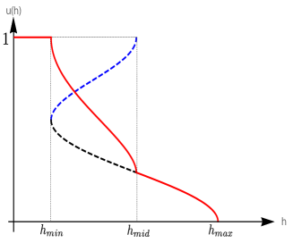
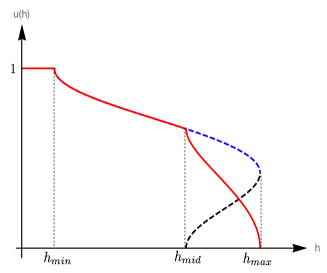
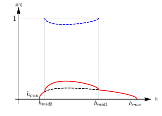
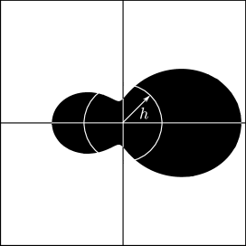
Since (h,θ)𝜃(h,\theta) are canonical conjugate of each other, integrating out θ𝜃\theta in phase space gives us momentum distribution for free fermions under consideration. Thus, momentum distribution is actually encoded in the arrangements of boxes in the most dominant Young tableaux. To obtain Young distribution function u(h)𝑢u(h) we use the definition (1.4). Unlike eigenvalue distribution, finding Young tableaux distribution directly from partition function is a formidable task for a generic matrix model. But we assume that the definition (1.4) holds in general. This definition boils down to our earlier identification [10, 11] πu(h)=θ𝜋𝑢𝜃\pi u(h)=\theta when θ𝜃\theta has unique solution for a given hh in equation (4.1). In general, θ𝜃\theta may have multiple solutions for a given hh. In that case u(h)𝑢u(h) is given by total length of different segments of white arc as shown in figure 2.
Refer to caption
Figure 2: u(h)𝑢u(h) is same the length of white line of radius hh for no-gap phase.

This equation is, in general, difficult to solve and find u(h)𝑢u(h) for any arbitrary set of parameters {βn}subscript𝛽𝑛\{\beta_{n}\}. In section 5 and 6 we use this relation to find the Young tableaux distribution which dominates the partition function in large N𝑁N limit.

Young distribution captures information about momentum distribution of N𝑁N fermions. Therefore, large N𝑁N state of the system can be found from Young distribution. Since fermions have momentum h1,,hNsubscript1subscript𝑁h_{1},\cdots,h_{N} a large N𝑁N state of the system can be recognised as |h1,,hNketsubscript1subscript𝑁|h_{1},\cdots,h_{N}\rangle in momentum space121212 We are considering a quantum mechanics on circle hence momenta of particles are integers.[2]. Thus a large N𝑁N state correspond to geometry of Young diagram. Time evolution of quantum fluctuations about this large N𝑁N states can be studied using underlying UMQM.

Finding dominant Young distributions is also important, as local dynamics of holographic geometry is encoded in Young diagram of dual theory [31]. Supersymmetry plays an important role here, as weak coupling results are protected. Hence, by determining phase space distribution and corresponding Young diagrams for a supersymmetry theory one can reconstruct the dual holographic geometry from that.

5 Young distribution for β1β2subscript𝛽1subscript𝛽2\beta_{1}-\beta_{2} model

In this section we discuss an example where we have non-trivial, stable two gap phases. This example will help us to understand how to reconstruct Young diagrams from phase space for different large N𝑁N phases of the theory.

To have a two gap solution we need the potential V(θ)𝑉𝜃V(\theta) in equation (2.5) to have two minima between π𝜋-\pi and π𝜋\pi. This is achieved by considering a plaquette model with β1,β20subscript𝛽1subscript𝛽20\beta_{1},\beta_{2}\neq 0 and βn=0forn3subscript𝛽𝑛0for𝑛3\beta_{n}=0\ \text{for}\ n\geq 3. The action S(U)𝑆𝑈S(U) is given by

S(U)𝑆𝑈\displaystyle\displaystyle{S(U)} =\displaystyle= N[β1(TrU+TrU)+β22(TrU2+TrU2)].𝑁delimited-[]subscript𝛽1Tr𝑈Trsuperscript𝑈subscript𝛽22Trsuperscript𝑈2Trsuperscript𝑈absent2\displaystyle N\left[\beta_{1}(\text{Tr}U+\text{Tr}U^{\dagger})+{\beta_{2}\over 2}(\text{Tr}U^{2}+\text{Tr}U^{\dagger 2})\right]. (5.1)

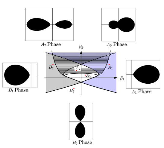
Phase structure of this model was discussed in [20] and [21]. The model exhibits ”five” different phases depending on values of parameters β1subscript𝛽1\beta_{1} and β2subscript𝛽2\beta_{2}: one no-gap phase, two one-gap phases (mirror reflection of each other) and two two-gap phases. A detailed derivation of eigenvalue distribution for different phases can be found in [20, 21]. Here, we present a different and independent method (solving Dyson-Schwinger equation) to reproduce the results (eigenvalue distribution) of [20, 21]. Then we obtain droplets for different phases of the theory. Finally, we discuss how to reconstruct Young tableaux distributions for five different phases of this model from the geometry of droplets.

5.1 The resolvent

Eigenvalue distribution can be obtained from analytic properties of resolvent which satisfies an algebraic equation in large N𝑁N limit [32]. This method is quite powerful as one does not need to solve an integral equation for eigenvalue density. We briefly review the method here.

“Resolvent” for any generic UMM (2.1) is defined as,

R(z)=N1Tr[(1zU)1]𝑅𝑧superscript𝑁1delimited-⟨⟩Trdelimited-[]superscript1𝑧𝑈1R(z)=N^{-1}\langle\text{Tr}[(1-zU)^{-1}]\rangle (5.2)

where z𝑧z is a complex variable. Expanding the right hand side of (5.2)

R(z)=1+1N(zTrU+z2TrU2+z3TrU3+).𝑅𝑧11𝑁𝑧delimited-⟨⟩Tr𝑈superscript𝑧2delimited-⟨⟩Trsuperscript𝑈2superscript𝑧3delimited-⟨⟩Trsuperscript𝑈3R(z)=1+\frac{1}{N}\left(z\langle\text{Tr}U\rangle+z^{2}\langle\text{Tr}U^{2}\rangle+z^{3}\langle\text{Tr}U^{3}\rangle+\cdots\right). (5.3)

One can see that the resolvent is a generating functional of Wilson loops in the planar limit. Since N1TrUksuperscript𝑁1delimited-⟨⟩Trsuperscript𝑈𝑘N^{-1}\langle\text{Tr}U^{k}\rangle lies between 11-1 and +11+1 the right hand side of equation (5.3) is convergent for |z|<1𝑧1|z|<1. Therefore, R(z)𝑅𝑧R(z) is an analytic and holomorphic function in the interior of the unit disk. In a similar way, one can show that the function R(z)𝑅𝑧R(z) is also analytic for |z|>1𝑧1|z|>1 with R(z)0𝑅𝑧0R(z)\rightarrow 0 for |z|𝑧|z|\rightarrow\infty. However, R(z)𝑅𝑧R(z) is discontinuous on |z|=1𝑧1|z|=1. Inside the unit circle one can also write that,

R(1/z)=zN1Tr[U1]z2N1Tr[U2]+,|z|<1.formulae-sequence𝑅1𝑧𝑧superscript𝑁1delimited-⟨⟩𝑇𝑟delimited-[]superscript𝑈1superscript𝑧2superscript𝑁1delimited-⟨⟩𝑇𝑟delimited-[]superscript𝑈2𝑧1\displaystyle R(1/z)=-zN^{-1}\langle Tr[U^{-1}]\rangle-z^{2}N^{-1}\langle Tr[U^{-2}]\rangle+\cdots,\quad|z|<1. (5.4)

Hence we have the following property of R(z)𝑅𝑧R(z)

R(z)+R(1/z)=1,for|z|1.formulae-sequence𝑅𝑧𝑅1𝑧1for𝑧1R(z)+R(1/z)=1,\quad\text{for}\quad|z|\neq 1. (5.5)

At large N the resolvent satisfies a quadratic equation (Dyson-Schwinger equation) which can be solved algebraically [11]. The solution, for a particular model (5.1) under consideration, is given by (see [11] for details)

R(z)=12[12+β1(z1z)+β2(z21z2)+F(z)]|z|<1𝑅𝑧12delimited-[]12subscript𝛽1𝑧1𝑧subscript𝛽2superscript𝑧21superscript𝑧2𝐹𝑧𝑧1\displaystyle R(z)={1\over 2}\left[{1\over 2}+\beta_{1}(z-{1\over z})+\beta_{2}(z^{2}-{1\over z^{2}})+\sqrt{F(z)}\right]\quad\text{$|z|<1$} (5.6)
R(z)=12[12+β1(z1z)+β2(z21z2)F(z)]|z|>1𝑅𝑧12delimited-[]12subscript𝛽1𝑧1𝑧subscript𝛽2superscript𝑧21superscript𝑧2𝐹𝑧𝑧1\displaystyle R(z)={1\over 2}\left[{1\over 2}+\beta_{1}(z-{1\over z})+\beta_{2}(z^{2}-{1\over z^{2}})-\sqrt{F(z)}\right]\quad\text{$|z|>1$} (5.7)

where F(z)𝐹𝑧F(z) has the following form,

F(z)=[β1(1z+z)+β2(1z2+z2)+1]24(β1z+β2z2)[β1z+β2z2]+4β1R(0)+4β2[R(0)z+R′′(0)2+R(0)z].𝐹𝑧superscriptdelimited-[]subscript𝛽11𝑧𝑧subscript𝛽21superscript𝑧2superscript𝑧2124subscript𝛽1𝑧subscript𝛽2superscript𝑧2delimited-[]subscript𝛽1𝑧subscript𝛽2superscript𝑧24subscript𝛽1superscript𝑅04subscript𝛽2delimited-[]superscript𝑅0𝑧superscript𝑅′′02superscript𝑅0𝑧\begin{split}F(z)&=\bigg{[}\beta_{1}\left(\frac{1}{z}+z\right)+\beta_{2}\left(\frac{1}{z^{2}}+z^{2}\right)+1\bigg{]}^{2}-4\left(\beta_{1}z+\beta_{2}z^{2}\right)\left[\frac{\beta_{1}}{z}+\frac{\beta_{2}}{z^{2}}\right]\\ &\hskip 102.43008pt+4\beta_{1}R^{\prime}(0)+4\beta_{2}\left[\frac{R^{\prime}(0)}{z}+\frac{R^{\prime\prime}(0)}{2}+R^{\prime}(0)z\right].\end{split} (5.8)

Spectral density or eigenvalue density is related to discontinuity of R(z)𝑅𝑧R(z) on unit circle. Eigenvalue distribution function (ρ(θ)𝜌𝜃\rho(\theta)) is given by,

2πρ(θ)=limϵ0[R((1+ϵ)eiθ)R((1ϵ)eiθ)]=2[R(eiθ)]1=F(eiθ).2𝜋𝜌𝜃subscriptitalic-ϵ0delimited-[]𝑅1italic-ϵsuperscript𝑒𝑖𝜃𝑅1italic-ϵsuperscript𝑒𝑖𝜃2𝑅superscript𝑒𝑖𝜃1𝐹superscript𝑒𝑖𝜃\displaystyle 2\pi\rho(\theta)=\lim_{\epsilon\to 0}\left[R((1+\epsilon)e^{i\theta})-R((1-\epsilon)e^{i\theta})\right]=2\Re\left[R(e^{i\theta})\right]-1=\sqrt{F(e^{i\theta})}. (5.9)

We see that F(z)𝐹𝑧F(z) contains some quantities R(0)superscript𝑅0R^{\prime}(0) and R′′(0)superscript𝑅′′0R^{\prime\prime}(0) which can be calculated from (5.6). Therefore one has to consistently solve these equations to find R(0)superscript𝑅0R^{\prime}(0) and R′′(0)superscript𝑅′′0R^{\prime\prime}(0) for different phases of the model and then ρ(θ)𝜌𝜃\rho(\theta) from (5.8). However, it is difficult to solve equation (5.6) and (5.8) consistently. Rather, we shall take an ansatz for F(z)𝐹𝑧F(z) for different phases of the theory and fix the form of F(z)𝐹𝑧F(z) from analytic properties of R(z)𝑅𝑧R(z) :

  1. 1.

    R(z)𝑅𝑧{R}(z) is analytic inside the unit circle. In equation (5.6) we see that R(z)𝑅𝑧R(z) has 1/z1𝑧1/z and 1/z21superscript𝑧21/z^{2} terms which are singular at z=0𝑧0z=0. Therefore, F(z)𝐹𝑧\sqrt{F(z)} should have poles of order one and two at z=0𝑧0z=0 to make R(z)𝑅𝑧R(z) analytic inside. F(z)𝐹𝑧F(z) can not have zeros inside (or outside) the unit circle. In that case F(z)𝐹𝑧\sqrt{F(z)} would have branch points inside or outside the circle. However, F(z)𝐹𝑧F(z) can have zeros on |z|=1𝑧1|z|=1 line.

  2. 2.

    For gapped solution F(z)𝐹𝑧\sqrt{F(z)} should have branch points on unit circle. Also F(z)𝐹𝑧F(z) is invariant under z1/z𝑧1𝑧z\to 1/z.

  3. 3.

    Finally, R(z)𝑅𝑧R(z) is normalized as R<(0)=1subscript𝑅01R_{<}(0)=1.

5.2 Large N𝑁N phases and eigenvalue distribution

No-gap solution

This is the most trivial case where there is no branch cuts in resolvent R(z)𝑅𝑧R(z). Hence, F(z)𝐹𝑧F(z) is a perfect square. Thus we have,

F(z)=[1+β1(z+1z)+β2(z2+1z2)]2.𝐹𝑧superscriptdelimited-[]1subscript𝛽1𝑧1𝑧subscript𝛽2superscript𝑧21superscript𝑧22F(z)=\left[1+\beta_{1}\left(z+{1\over z}\right)+\beta_{2}\left(z^{2}+{1\over z^{2}}\right)\right]^{2}. (5.10)

The eigenvalue distribution for this phase is given by (from equation 5.9)

ρA0(θ)=12π(1+2β1cosθ+2β2cos2θ)subscript𝜌subscript𝐴0𝜃12𝜋12subscript𝛽1𝜃2subscript𝛽22𝜃\rho_{A_{0}}(\theta)={1\over 2\pi}(1+2\beta_{1}\cos\theta+2\beta_{2}\cos 2\theta) (5.11)

for 0θ2π0𝜃2𝜋0\leq\theta\leq 2\pi.

Since ρ(θ)0𝜌𝜃0\rho(\theta)\geq 0, a no-gap or zero-gap solution exists for [20]

β124β2(12β2)=0,forβ216|β1|β212=0,for12β216\displaystyle\displaystyle\begin{split}\beta_{1}^{2}-4\beta_{2}(1-2\beta_{2})&=0,\quad\text{for}\quad\beta_{2}\geq\frac{1}{6}\\ |\beta_{1}|-\beta_{2}-\frac{1}{2}&=0,\quad\text{for}\quad-\frac{1}{2}\leq\beta_{2}\leq\frac{1}{6}\end{split} (5.12)

We use the notation of [20] to name different phases of this model. No-gap phase is called A0subscript𝐴0A_{0} phase. Note that there is a factor of 222 difference between our set of parameters and [20]’s set of parameters : (2β1, 2β2)our=(β1,β2)[20]subscript2subscript𝛽12subscript𝛽2oursubscriptsubscript𝛽1subscript𝛽2[20](2\beta_{1},\ 2\beta_{2})_{\text{our}}=(\beta_{1},\ \beta_{2})_{\text{\cite[cite]{[\@@bibref{}{zalewski}{}{}]}}}.

One-gap solution

For one-gap solution F(z)𝐹𝑧\sqrt{F(z)} has a branch cut on |z|=1𝑧1|z|=1. Therefore the most generic ansatz for F(z)𝐹𝑧F(z) for one-gap phase is given by,

F(z)=α(z+1z)γ+(z+1z)2[β+(z+1z)2],𝐹𝑧𝛼𝑧1𝑧𝛾superscript𝑧1𝑧2delimited-[]𝛽superscript𝑧1𝑧2\displaystyle\sqrt{F(z)}=\alpha\left(\sqrt{z}+\frac{1}{\sqrt{z}}\right)\sqrt{\gamma+\left(\sqrt{z}+\frac{1}{\sqrt{z}}\right)^{2}}\left[\beta+\left(\sqrt{z}+\frac{1}{\sqrt{z}}\right)^{2}\right], (5.13)

where α,β,γare constants𝛼𝛽𝛾are constants\alpha,\ \beta,\ \gamma\ \text{are constants}. From analyticity and normalization condition of R(z)𝑅𝑧R(z) we find

α=β2;β=β1β2γ24;γ=23β(β14β2+6β2+(β1+2β2)2).formulae-sequence𝛼subscript𝛽2formulae-sequence𝛽subscript𝛽1subscript𝛽2𝛾24𝛾23𝛽subscript𝛽14subscript𝛽26subscript𝛽2superscriptsubscript𝛽12subscript𝛽22\displaystyle\alpha=\beta_{2};\quad\beta={\beta_{1}\over\beta_{2}}-{\gamma\over 2}-4;\quad\gamma={2\over 3\beta}\left(\beta_{1}-4\beta_{2}+\sqrt{-6\beta_{2}+(\beta_{1}+2\beta_{2})^{2}}\right). (5.14)

Hence, the spectral density for one-gap solution (A1subscript𝐴1A_{1} phase) is given by

ρA1(θ)=2πsin2θ12sin2θ2cosθ2[β1+β2(2cosθ+cosθ11)],subscript𝜌subscript𝐴1𝜃2𝜋superscript2subscript𝜃12superscript2𝜃2𝜃2delimited-[]subscript𝛽1subscript𝛽22𝜃subscript𝜃11\displaystyle\rho_{A_{1}}(\theta)={2\over\pi}\sqrt{\sin^{2}{\theta_{1}\over 2}-\sin^{2}{\theta\over 2}}\cos{\theta\over 2}\left[\beta_{1}+\beta_{2}(2\cos\theta+\cos\theta_{1}-1)\right], (5.15)

with

sin2θ12=β1+2β26β2+(β1+2β2)26β2.superscript2subscript𝜃12subscript𝛽12subscript𝛽26subscript𝛽2superscriptsubscript𝛽12subscript𝛽226subscript𝛽2\sin^{2}{\theta_{1}\over 2}={\beta_{1}+2\beta_{2}-\sqrt{-6\beta_{2}+(\beta_{1}+2\beta_{2})^{2}}\over 6\beta_{2}}. (5.16)

Eigenvalues are symmetrically distributed about θ=0𝜃0\theta=0 from θ1subscript𝜃1-\theta_{1} to θ1subscript𝜃1\theta_{1}. One-gap solution is valid in the following region in (β1,β2)subscript𝛽1subscript𝛽2(\beta_{1},\beta_{2}) plane bounded by the curves [20]

(β1+2β2)26β2=0,forβ216,β1β212=0,for12β216,(β1+2β2)2+2β2=0,forβ212\displaystyle\displaystyle\begin{split}(\beta_{1}+2\beta_{2})^{2}-6\beta_{2}&=0,\quad\text{for}\quad\beta_{2}\geq\frac{1}{6},\\ \beta_{1}-\beta_{2}-\frac{1}{2}&=0,\quad\text{for}\quad-\frac{1}{2}\leq\beta_{2}\leq\frac{1}{6},\\ (\beta_{1}+2\beta_{2})^{2}+2\beta_{2}&=0,\quad\text{for}\quad\beta_{2}\leq-\frac{1}{2}\end{split} (5.17)

and extends in the direction of positive β1subscript𝛽1\beta_{1}. There exists a common boundary between this phase and zero-gap phase and is given by

β1=β2+1,for12β216.formulae-sequencesubscript𝛽1subscript𝛽21for12subscript𝛽216\beta_{1}=\beta_{2}+1,\quad\text{for}\quad-\frac{1}{2}\leq\beta_{2}\leq\frac{1}{6}. (5.18)

F(z)𝐹𝑧F(z) (given by equation 5.13) for one-gap solution has a branch cut on unit circle about z=1𝑧1z=1 point (θ=0𝜃0\theta=0). If we replace z𝑧z by z𝑧-z then the branch-cut changes its position from right to left side on the unit circle. However, this is also a valid ansatz for F(z)𝐹𝑧F(z) for one-gap solution (B1subscript𝐵1B_{1} phase). For this ansatz the parameters α,β,γ𝛼𝛽𝛾\alpha,\beta,\gamma take the following values to make R(z)𝑅𝑧R(z) analytic inside.

α=β2;β=β1β2γ24;γ=23β(β14β2+6β2+(β1+2β2)2),formulae-sequence𝛼subscript𝛽2formulae-sequence𝛽subscript𝛽1subscript𝛽2𝛾24𝛾23𝛽subscript𝛽14subscript𝛽26subscript𝛽2superscriptsubscript𝛽12subscript𝛽22\displaystyle\alpha=\beta_{2};\quad\beta=-{\beta_{1}\over\beta_{2}}-{\gamma\over 2}-4;\quad\gamma={2\over 3\beta}\left(-\beta_{1}-4\beta_{2}+\sqrt{-6\beta_{2}+(-\beta_{1}+2\beta_{2})^{2}}\right), (5.19)

which in turn gives the spectral density as

ρB1(θ)=2πcos2θ12cos2θ2sinθ2[β1β2(2cosθ+cosθ1+1)],subscript𝜌subscript𝐵1𝜃2𝜋superscript2subscript𝜃12superscript2𝜃2𝜃2delimited-[]subscript𝛽1subscript𝛽22𝜃subscript𝜃11\displaystyle\rho_{B_{1}}(\theta)={2\over\pi}\sqrt{\cos^{2}{\theta_{1}\over 2}-\cos^{2}{\theta\over 2}}\,\sin{\theta\over 2}\,\left[\beta_{1}-\beta_{2}(2\cos\theta+\cos\theta_{1}+1)\right], (5.20)

with

cos2θ2=β1+2β26β2+(β1+2β2)26β2.superscript2𝜃2subscript𝛽12subscript𝛽26subscript𝛽2superscriptsubscript𝛽12subscript𝛽226subscript𝛽2\cos^{2}{\theta\over 2}={-\beta_{1}+2\beta_{2}-\sqrt{-6\beta_{2}+(-\beta_{1}+2\beta_{2})^{2}}\over 6\beta_{2}}. (5.21)

Since action (5.1) is invariant under β1β1subscript𝛽1subscript𝛽1\beta_{1}\rightarrow-\beta_{1} and θθ+π𝜃𝜃𝜋\theta\rightarrow\theta+\pi therefore, it is expected that there exists a mirror image of A1subscript𝐴1A_{1} phase in negative β1subscript𝛽1\beta_{1} direction (B1subscript𝐵1B_{1} phase). Eigenvalues, for this branch, are distributed symmetrically about θ=π𝜃𝜋\theta=\pi from π+|θ1|𝜋subscript𝜃1\pi+|\theta_{1}| to π|θ1|𝜋subscript𝜃1\pi-|\theta_{1}|. Similarly, the common boundary between this phase and zero-gap phase is given by

β1=β21,for12β216.formulae-sequencesubscript𝛽1subscript𝛽21for12subscript𝛽216\beta_{1}=-\beta_{2}-1,\quad\text{for}\quad-\frac{1}{2}\leq\beta_{2}\leq\frac{1}{6}. (5.22)

A transition along line (5.18) or (5.22) between zero-gap and one-gap (or its mirror phase) is a third order phase transition. This is a generalization of Gross-Witten-Wadia transition [33, 34]. In subsection 5.3 we shall see how phase space topology changes as we go from one phase to another.

Two-gap solution

To have a two-gap solution one should take an ansatz for F(z)𝐹𝑧\sqrt{F(z)} such that there is at most a degree four polynomial inside the square root. In this case there are two possible ways of taking ansatz for F(z)𝐹𝑧F(z) which give two different two-gap phases namely A2subscript𝐴2A_{2} phase and B2subscript𝐵2B_{2} phase.

A2subscript𝐴2A_{2} Phase

The simplest ansatz that one can take is

F(z)=α2(z+1z)2+β(z+1z)+1(δ+σ(z+1z)).𝐹𝑧superscript𝛼2superscript𝑧1𝑧2𝛽𝑧1𝑧1𝛿𝜎𝑧1𝑧\sqrt{F(z)}=\sqrt{\alpha^{2}\left(z+{1\over z}\right)^{2}+\beta\left(z+{1\over z}\right)+1}\,\left(\delta+\sigma\left(z+{1\over z}\right)\right). (5.23)

α,β,σ,δ𝛼𝛽𝜎𝛿\alpha,\beta,\sigma,\delta are constants. Using the analyticity and normalization condition of R(z)𝑅𝑧R(z) we find,

σ=β2α;δ=2α2β1ββ22α3;α2=ββ1β2+2ββ1β2+β22+β2(β12+6β2(1+2β2))4+8β2.formulae-sequence𝜎subscript𝛽2𝛼formulae-sequence𝛿2superscript𝛼2subscript𝛽1𝛽subscript𝛽22superscript𝛼3superscript𝛼2𝛽subscript𝛽1subscript𝛽22𝛽subscript𝛽1subscript𝛽2superscriptsubscript𝛽22superscript𝛽2superscriptsubscript𝛽126subscript𝛽212subscript𝛽248subscript𝛽2\displaystyle\sigma={\beta_{2}\over\alpha};\quad\delta={2\alpha^{2}\beta_{1}-\beta\beta_{2}\over 2\alpha^{3}};\quad\alpha^{2}=\displaystyle{{-\beta\beta_{1}-\beta_{2}+\sqrt{2\beta\beta_{1}\beta_{2}+\beta_{2}^{2}+\beta^{2}\left(\beta_{1}^{2}+6\beta_{2}(-1+2\beta_{2})\right)}\over-4+8\beta_{2}}}.

However, it is not possible to fix all the four parameters from the properties of R(z)𝑅𝑧R(z). We keep β𝛽\beta undetermined. The eigenvalue distribution in this case is given by,

ρA2(θ)=1π(cosθcosθ1)(cosθcosθ2)[β1+β2(2cosθ+cosθ1+cosθ2)]subscript𝜌subscript𝐴2𝜃1𝜋𝜃subscript𝜃1𝜃subscript𝜃2delimited-[]subscript𝛽1subscript𝛽22𝜃subscript𝜃1subscript𝜃2\displaystyle\rho_{A_{2}}(\theta)={1\over\pi}\sqrt{(\cos\theta-\cos\theta_{1})(\cos\theta-\cos\theta_{2})}\,\,\,\,\left[\beta_{1}+\beta_{2}(2\cos\theta+\cos\theta_{1}+\cos\theta_{2})\right]

where

cosθ1=β4α14α4α+β2;cosθ2=β4α+14α4α+β2.formulae-sequencesubscript𝜃1𝛽4𝛼14𝛼4𝛼superscript𝛽2subscript𝜃2𝛽4𝛼14𝛼4𝛼superscript𝛽2\displaystyle\cos\theta_{1}=-{\beta\over 4\alpha}-{1\over 4\alpha}\sqrt{-4\alpha+\beta^{2}};\quad\cos\theta_{2}=-{\beta\over 4\alpha}+{1\over 4\alpha}\sqrt{-4\alpha+\beta^{2}}. (5.26)

A2subscript𝐴2A_{2} phase has eigenvalue distribution symmetric about horizontal axis. Validity of this phase has been shown in figure 3. Eigenvalues are distributed between θ1subscript𝜃1-\theta_{1} and θ1subscript𝜃1\theta_{1} and then πθ2𝜋subscript𝜃2\pi-\theta_{2} to π+θ2𝜋subscript𝜃2\pi+\theta_{2}.

Eliminating the undetermined parameter β𝛽\beta from equations (5.26) one can write a constraint equation relating cosθ1subscript𝜃1\cos\theta_{1} and cosθ2subscript𝜃2\cos\theta_{2} as

β1(cosθ1+cosθ2)+β2[2(cosθ1+cosθ2)212(cosθ1cosθ2)2]=1.subscript𝛽1subscript𝜃1subscript𝜃2subscript𝛽2delimited-[]2superscriptsubscript𝜃1subscript𝜃2212superscriptsubscript𝜃1subscript𝜃221\displaystyle-\beta_{1}(\cos\theta_{1}+\cos\theta_{2})+\beta_{2}\left[2-(\cos\theta_{1}+\cos\theta_{2})^{2}-{1\over 2}(\cos\theta_{1}-\cos\theta_{2})^{2}\right]=1. (5.27)

The undetermined parameter β𝛽\beta can be fixed by imposing an extra condition that total number of eigenvalues between θ1subscript𝜃1\theta_{1} and θ2subscript𝜃2\theta_{2} is zero

1πθ1θ2ρA2(θ)𝑑θ=0.1𝜋superscriptsubscriptsubscript𝜃1subscript𝜃2subscript𝜌subscript𝐴2𝜃differential-d𝜃0\frac{1}{\pi}\int_{\theta_{1}}^{\theta_{2}}\rho_{A_{2}}(\theta)d\theta=0. (5.28)

A second order phase transition between A2subscript𝐴2A_{2} phase and A1subscript𝐴1A_{1} phase (or B1subscript𝐵1B_{1} phase) occurs along the lines [20]

β2=14cos3θ1[cos12θ1sin2θ1ln(1+cos12θ1sinθ1)],β1=12sin2θp2[12β2sin212θ1(23sin212θ1)].formulae-sequencesubscript𝛽214superscript3subscript𝜃1delimited-[]12subscript𝜃1superscript2subscript𝜃1112subscript𝜃1subscript𝜃1subscript𝛽112superscript2subscript𝜃𝑝2delimited-[]12subscript𝛽2superscript212subscript𝜃123superscript212subscript𝜃1\displaystyle\displaystyle\begin{split}\beta_{2}&=\frac{1}{4\cos^{3}\theta_{1}}\left[{\cos\frac{1}{2}\theta_{1}\over\sin^{2}\theta_{1}}-\ln\left(\frac{1+\cos\frac{1}{2}\theta_{1}}{\sin\theta_{1}}\right)\right],\\ \beta_{1}&=\frac{1}{2\sin^{2}\frac{\theta_{p}}{2}}\left[1-2\beta_{2}\sin^{2}\frac{1}{2}\theta_{1}(2-3\sin^{2}\frac{1}{2}\theta_{1})\right].\end{split} (5.29)

B2subscript𝐵2B_{2} Phase

The second possible ansatz for F(z)𝐹𝑧F(z) for a two gap solution is given by,

F(z)=γ(z+1z)24α2(z+1z)2+β(z+1z)+1.𝐹𝑧𝛾superscript𝑧1𝑧24superscript𝛼2superscript𝑧1𝑧2𝛽𝑧1𝑧1\sqrt{F(z)}=\gamma\sqrt{\left(z+\frac{1}{z}\right)^{2}-4}\,\,\,\,\sqrt{\alpha^{2}\left(z+{1\over z}\right)^{2}+\beta\left(z+{1\over z}\right)+1}. (5.30)

with,

α2=β22β12+2β2;β=2β1β2β12+2β2;γ=2iβ12+2β2.formulae-sequencesuperscript𝛼2superscriptsubscript𝛽22superscriptsubscript𝛽122subscript𝛽2formulae-sequence𝛽2subscript𝛽1subscript𝛽2superscriptsubscript𝛽122subscript𝛽2𝛾2𝑖superscriptsubscript𝛽122subscript𝛽2\displaystyle\alpha^{2}={\beta_{2}^{2}\over\beta_{1}^{2}+2\beta_{2}};\quad\beta={2\beta_{1}\beta_{2}\over\beta_{1}^{2}+2\beta_{2}};\quad\gamma=-2\,i\,\sqrt{\beta_{1}^{2}+2\beta_{2}}. (5.31)

The spectral density for this case is

ρ(θ)=2β2π|sinθ|(cosθ1cosθ)(cosθcosθ2)𝜌𝜃2subscript𝛽2𝜋𝜃subscript𝜃1𝜃𝜃subscript𝜃2\displaystyle\rho(\theta)=-{2\beta_{2}\over\pi}|\sin\theta|\sqrt{(\cos\theta_{1}-\cos\theta)(\cos\theta-\cos\theta_{2})} (5.32)

with

cosθ1=β12β2+12β2;cosθ2=β12β212β2.formulae-sequencesubscript𝜃1subscript𝛽12subscript𝛽212subscript𝛽2subscript𝜃2subscript𝛽12subscript𝛽212subscript𝛽2\displaystyle\cos\theta_{1}=-{\beta_{1}\over 2\beta_{2}}+\sqrt{-1\over 2\beta_{2}};\quad\cos\theta_{2}=-{\beta_{1}\over 2\beta_{2}}-\sqrt{-1\over 2\beta_{2}}. (5.33)

Eigenvalues are distributed between θ1subscript𝜃1\theta_{1} and θ2subscript𝜃2\theta_{2}, and θ1subscript𝜃1-\theta_{1} and θ2subscript𝜃2-\theta_{2}. This phase exists for β213subscript𝛽213\beta_{2}\leq-\frac{1}{3}. A parabola (β1+2β2)2+4β2=0superscriptsubscript𝛽12subscript𝛽224subscript𝛽20(-\beta_{1}+2\beta_{2})^{2}+4\beta_{2}=0 separates this phase from one-gap phase. The point (β1=0,β2=12)formulae-sequencesubscript𝛽10subscript𝛽212(\beta_{1}=0,\beta_{2}=-\frac{1}{2}) is a triple point in the parameter space. See figure (3) for details.

5.3 Droplets and phase transition in β1β2subscript𝛽1subscript𝛽2\beta_{1}-\beta_{2} model

We shall discuss about geometries of droplets for different phases of the model. The boundary relation (3.38) for this model is given by

h±(θ)=12+β1cosθ+β2cos2θ±πρ(θ)subscriptplus-or-minus𝜃plus-or-minus12subscript𝛽1𝜃subscript𝛽22𝜃𝜋𝜌𝜃h_{\pm}(\theta)=\frac{1}{2}+\beta_{1}\cos{\theta}+\beta_{2}\cos 2\theta\pm\pi\rho(\theta) (5.34)

where h±(θ)subscriptplus-or-minus𝜃h_{\pm}(\theta) are solutions of

h2(1+β1cosθ+β2cos2θ)h=π2ρ2(θ).superscript21subscript𝛽1𝜃subscript𝛽22𝜃superscript𝜋2superscript𝜌2𝜃h^{2}-\left(1+\beta_{1}\cos{\theta}+\beta_{2}\cos 2\theta\right)h=\pi^{2}\rho^{2}(\theta). (5.35)
Refer to caption
Figure 3: Droplets for β1β2subscript𝛽1subscript𝛽2\beta_{1}-\beta_{2} model. The central figure shows parameter space of the model. All the distributions are plotted in polar coordinates (h,θ)𝜃(h,\theta), hh radial and θ𝜃\theta angular. The black regions correspond to density ω(h,θ)=1𝜔𝜃1\omega(h,\theta)=1. Figure on top right shows droplet for no gap phase. Here we see that distribution is non-zero for all values of θ𝜃\theta. This implies eigenvalue density is non-zero for all values of θ𝜃\theta and hence the name no-gap (in eigenvalues) phase. Distribution on right middle corresponds to one-gap phase A1subscript𝐴1A_{1}. Unlike no-gap phase, here distribution is non-zero for θ𝜃\theta between θ1subscript𝜃1-\theta_{1} and θ1subscript𝜃1\theta_{1}. Distribution at the bottom correspond to B2subscript𝐵2B_{2} phase. Here, distribution is non-zero for θ𝜃\theta between two different ranges. Distribution on left middle is a mirror image of A1subscript𝐴1A_{1} phase. This is B1subscript𝐵1B_{1} phase. Finally, on top left we draw distribution for the second two-gap phase (A2subscript𝐴2A_{2}). Here also phase space density is non-zero for two different ranges of θ𝜃\theta. One should note that all the distributions are symmetric about θ=0𝜃0\theta=0 line. This is because of UU𝑈superscript𝑈U\rightarrow U^{\dagger} symmetry of the model.

There are five possible droplets with different topologies corresponding to five different phases. In figure 3 we draw phase space distributions for different phases. The diagram in the middle is parameter space (β1β2subscript𝛽1subscript𝛽2\beta_{1}-\beta_{2} plane) of the theory under consideration. We divide this parameter space into different parts according to validity of different phases. See [20] for more detail131313The parameter space in 3 is similar to the parameter space given in [20]. However, it has been re-drawn according to our normalization.. Since, h>00h>0 (being number of boxes) and π<θπ𝜋𝜃𝜋-\pi<\theta\leq\pi, we plot phase space distribution in polar coordinates. The black regions correspond to density ω(h,θ)=1𝜔𝜃1\omega(h,\theta)=1. We note that topologies of droplets are different for different phases. Origin (h=00h=0) is inside the distribution for no-gap phase (since h(θ)subscript𝜃h_{-}(\theta) is zero for all θ𝜃\theta). For one-gap and two-gap phases, on the other hand, origin is outside the distribution (both h+subscripth_{+} and hsubscripth_{-} are non-zero). We consider this as a topological property of droplets. One should also note that all the distributions are symmetric about real axis (θ=0𝜃0\theta=0 line). This is because of UMM has UU𝑈superscript𝑈U\rightarrow U^{\dagger} symmetry. While deforming the droplets (by changing values of parameters) this symmetry is always preserved. Therefore, one can not continuously deform the droplets of B2subscript𝐵2B_{2} phase to bring them in the shape of droplets of A2subscript𝐴2A_{2} phase. This implies, there is no transition possible between B2subscript𝐵2B_{2} and A2subscript𝐴2A_{2} phases, which is true for this model. Boundary of a droplet crossing the origin implies (according to our definition) change of topology, which can only happen at the time of phase transition.
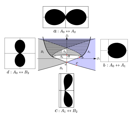
Refer to caption
Figure 4: Droplets for β1β2subscript𝛽1subscript𝛽2\beta_{1}-\beta_{2} model at different phase transition points.

We see that at A0subscript𝐴0A_{0}-A1subscript𝐴1A_{1} transition point (generalized Gross-Witten-Wadia transition), left boundary of the droplet touches the origin (figure 4(b)). From this point as we move towards A0subscript𝐴0A_{0}, the origin goes inside and as we move towards A1subscript𝐴1A_{1} the origin goes outside. Similarly, cutting a single droplet into two (or gluing two droplets to make a single one) also corresponds to change of topology and occurs at the time of phase transitions. For example, starting from A1subscript𝐴1A_{1} as we move towards B2subscript𝐵2B_{2} phase we see that A1subscript𝐴1A_{1} droplet starts deforming (two mid-points come closer) and finally becomes two blobs touching each other at a point (as shown in figure 4(c)) at the transition point. After that as we move in B2subscript𝐵2B_{2} region two blobs separate out from each other. Similar things happen for other transitions. Figure 4(d), 4(a) show distributions at A0B2subscript𝐴0subscript𝐵2A_{0}-B_{2} and A0A2subscript𝐴0subscript𝐴2A_{0}-A_{2} transition respectively.

Since boundary of droplets are fermi surfaces in underlying MQM, the above diagrams show how shape of fermi surfaces change during phase transition.

5.4 Reconstruction of Young diagrams from droplet geometry

The phase space description is a powerful approach as the shape of different droplets not only contains information about eigenvalue distributions but it also contains information about dominant representations for different phases of the theory. In this section we discuss how one can construct dominant Young diagrams for different phases.

To construct Young tableaux distribution from geometry of droplets we use equation (1.4). [10, 11], considered plaquette model with βn=0subscript𝛽𝑛0\beta_{n}=0 for n2𝑛2n\geq 2 and observed that while solving boundary relation (3.15) for a given hh there exists a unique value of θ𝜃\theta and hence Young distribution was given by πu(h)=θ(h)𝜋𝑢𝜃\pi u(h)=\theta(h) for all phases. However, solution for θ𝜃\theta does not remain unique when we turn on β2subscript𝛽2\beta_{2} in plaquette model (5.1). Here we see that boundary relation (5.35) for a fixed hh has maximum two possible solution for θ𝜃\theta. Therefore, the simple identification between eigenvalue and Young density (πu(h)=θ𝜋𝑢𝜃\pi u(h)=\theta) does not hold in this case. However, we consider equation (1.4) as a fundamental definition for u(h)𝑢u(h) and construct Young distributions from phase space for different phases.

No-gap phase

For no-gap phase ρ(θ)𝜌𝜃\rho(\theta) is given by (5.11). Therefore the Fermi surface for this phase is given by,

h+(θ)=1+2β1cosθ+2β2cos2θ,h(θ)=0.formulae-sequencesubscript𝜃12subscript𝛽1𝜃2subscript𝛽22𝜃subscript𝜃0h_{+}(\theta)=1+2\beta_{1}\cos\theta+2\beta_{2}\cos 2\theta,\quad h_{-}(\theta)=0. (5.36)

This defines a droplet about the origin. For β1>|4β2|subscript𝛽14subscript𝛽2\beta_{1}>|4\beta_{2}|, θ𝜃\theta has a unique solution (we denote that by θ¯1(h)subscript¯𝜃1\bar{\theta}_{1}(h)). In that case u(h)𝑢u(h) is given by

u(h)=θ¯1(h)2π,forβ1>|4β2|formulae-sequence𝑢subscript¯𝜃12𝜋forsubscript𝛽14subscript𝛽2u(h)=\frac{\bar{\theta}_{1}(h)}{2\pi},\quad\text{for}\quad\beta_{1}>|4\beta_{2}| (5.37)

as before.

For β1<|4β2|subscript𝛽14subscript𝛽2\beta_{1}<|4\beta_{2}|, θ𝜃\theta has multiple solutions depending on hh. In figure 5 we plot hh vs θ𝜃\theta for no-gap phase and for β1<|4β2|subscript𝛽14subscript𝛽2\beta_{1}<|4\beta_{2}|. The left and right plots correspond to positive and negative β2subscript𝛽2\beta_{2} respectively.

Refer to caption
(a) β2>0subscript𝛽20\beta_{2}>0
Refer to caption
(b) β2<0subscript𝛽20\beta_{2}<0
Figure 5: hh vs θ𝜃\theta for no-gap phase for β1<4|β2|subscript𝛽14subscript𝛽2\beta_{1}<4|\beta_{2}|. The black line correspond to h+(θ)subscript𝜃h_{+}(\theta).

Following definition (1.4), Young distribution for positive β2subscript𝛽2\beta_{2} is given by

u(h)=θ¯1(h)πforhmidhhmax=1θ¯2θ¯1πforhminhhmid.formulae-sequenceformulae-sequence𝑢subscript¯𝜃1𝜋forsubscript𝑚𝑖𝑑subscript𝑚𝑎𝑥1subscript¯𝜃2subscript¯𝜃1𝜋forsubscript𝑚𝑖𝑛subscript𝑚𝑖𝑑\displaystyle\displaystyle\begin{split}u(h)&={\bar{\theta}_{1}(h)\over\pi}\hskip 42.67912pt\text{for}\quad h_{mid}\leq h\leq h_{max}\\ &=1-\frac{\bar{\theta}_{2}-\bar{\theta}_{1}}{\pi}\hskip 15.6491pt\text{for}\quad h_{min}\leq h\leq h_{mid}.\end{split} (5.38)

For negative β2subscript𝛽2\beta_{2} the distribution is given by,

u(h)=θ¯2(h)θ¯1(h)πforhmidhhmax=θ¯2(h)πforhminhhmid.formulae-sequenceformulae-sequence𝑢subscript¯𝜃2subscript¯𝜃1𝜋forsubscript𝑚𝑖𝑑subscript𝑚𝑎𝑥subscript¯𝜃2𝜋forsubscript𝑚𝑖𝑛subscript𝑚𝑖𝑑\displaystyle\displaystyle\begin{split}u(h)&={\bar{\theta}_{2}(h)-\bar{\theta}_{1}(h)\over\pi}\hskip 14.22636pt\text{for}\quad h_{mid}\leq h\leq h_{max}\\ &=\frac{\bar{\theta}_{2}(h)}{\pi}\hskip 51.21504pt\text{for}\quad h_{min}\leq h\leq h_{mid}.\end{split} (5.39)

These definitions geometrically imply that u(h)𝑢u(h) is given by the length of the white arc of radius hh in figure 2 as discussed in section (4.2). Young distribution u(h)𝑢u(h) as a function of hh is shown in figure 6 for both positive and negative β2subscript𝛽2\beta_{2} and β1<4|β2|subscript𝛽14subscript𝛽2\beta_{1}<4|\beta_{2}|.

Refer to caption
(a) β2>0subscript𝛽20\beta_{2}>0
Refer to caption
(b) β2<0subscript𝛽20\beta_{2}<0
Figure 6: Young tableaux distribution for no-gap phase of β1β2subscript𝛽1subscript𝛽2\beta_{1}-\beta_{2} model. Blue and black dotted lines are θ¯2subscript¯𝜃2\bar{\theta}_{2} and θ¯1subscript¯𝜃1\bar{\theta}_{1} respectively. Red line depicts u(h)𝑢u(h).

We see that, there is a kink in the distribution. This correspond to sudden change in distribution function for boxes in a diagram. As in [10], Young tableaux for no-gap phase has finite number of rows empty. n(x)=0𝑛𝑥0n(x)=0 for 1<x<1hmin1𝑥1subscript𝑚𝑖𝑛1<x<1-h_{min}. After that number of boxes starts increasing and reaches a maximum value n(0)=hmax1𝑛0subscript𝑚𝑎𝑥1n(0)=h_{max}-1. The distribution of boxes from x=0𝑥0x=0 to x=1hmin𝑥1subscript𝑚𝑖𝑛x=1-h_{min} is governed by u(h)𝑢u(h) given by equation (5.38 or 5.39). Here we see a kink at h=hmidsubscript𝑚𝑖𝑑h=h_{mid}. For 0<h<hmin0subscript𝑚𝑖𝑛0<h<h_{min}, u(h)=1𝑢1u(h)=1.

Refer to caption
Figure 7: A typical Young tableaux for no-gap phase. Dotted line correspond to edge of the distribution of boxes in large N𝑁N limit. A kink corresponds to u(h)superscript𝑢u^{\prime}(h) is discontinuous.

A typical Young diagram for no-gap phase has been shown in figure 7. For negative values of β1subscript𝛽1\beta_{1} the story remains the same.

One-gap phase

Eigenvalue distribution for one-gap phase is given by equation (5.15). Boundary of phase space droplet is determined by equation (5.35) with ρ𝜌\rho replaced by ρA1subscript𝜌subscript𝐴1\rho_{A_{1}}. In figure 8 we plot hh vs. θ𝜃\theta for one-gap phase.

Refer to caption
(a) β1,β2>0subscript𝛽1subscript𝛽20\beta_{1},\beta_{2}>0 or β2<0subscript𝛽20\beta_{2}<0, β1>4|β2|subscript𝛽14subscript𝛽2\beta_{1}>4|\beta_{2}|.
Refer to caption
(b) β2<0subscript𝛽20\beta_{2}<0, β1<4|β2|subscript𝛽14subscript𝛽2\beta_{1}<4|\beta_{2}|.
Figure 8: Young tableaux distribution for one-gap phase of β1β2subscript𝛽1subscript𝛽2\beta_{1}-\beta_{2} model. Blue and black lines are h(θ)subscript𝜃h_{-}(\theta) and h+(θ)subscript𝜃h_{+}(\theta) lines respectively.

Here we see that for β1,β2>0subscript𝛽1subscript𝛽20\beta_{1},\beta_{2}>0 or β1>4|β2|subscript𝛽14subscript𝛽2\beta_{1}>4|\beta_{2}| for β2<0subscript𝛽20\beta_{2}<0 there is only one solution to θ𝜃\theta for a given hh (figure 8(a)). For β2<0subscript𝛽20\beta_{2}<0 two solutions of θ𝜃\theta develop for β1<4|β2|subscript𝛽14subscript𝛽2\beta_{1}<4|\beta_{2}| (figure 8(b)). Corresponding Young distributions are plotted in figure 9.
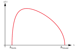
Refer to caption
(a) β1,β2>0subscript𝛽1subscript𝛽20\beta_{1},\beta_{2}>0 or β2<0subscript𝛽20\beta_{2}<0, β1>4|β2|subscript𝛽14subscript𝛽2\beta_{1}>4|\beta_{2}|.
Refer to caption
(b) β2<0subscript𝛽20\beta_{2}<0, β1<4|β2|subscript𝛽14subscript𝛽2\beta_{1}<4|\beta_{2}|.
Figure 9: Young tableaux distribution for one-gap phase of β1β2subscript𝛽1subscript𝛽2\beta_{1}-\beta_{2} model. Blue and black dotted lines are θ¯2subscript¯𝜃2\bar{\theta}_{2} and θ¯1subscript¯𝜃1\bar{\theta}_{1} respectively. Red line depicts u(h)𝑢u(h).

Young diagrams have all the rows filled with 𝒪(N)𝒪𝑁\mathcal{O}(N) number of boxes. The last row and the first row have Nhmin𝑁subscript𝑚𝑖𝑛Nh_{min} and N(hmax1)𝑁subscript𝑚𝑎𝑥1N(h_{max}-1) number of boxes respectively. In the first case (figure 9(a)), number of boxes smoothly increases from the last row to first row. In second case (figure 9(b)), we see that there is a kink in the Young diagram, figure 10.

Refer to caption
(a) β1,β2>0subscript𝛽1subscript𝛽20\beta_{1},\beta_{2}>0 or β1>4|β2|subscript𝛽14subscript𝛽2\beta_{1}>4|\beta_{2}| for β2<0subscript𝛽20\beta_{2}<0. The dotted black line denotes a smooth distribution of boxes. u(h)superscript𝑢u^{\prime}(h) is continuous everywhere.
Refer to caption
(b) β2<0subscript𝛽20\beta_{2}<0, β1<4|β2|subscript𝛽14subscript𝛽2\beta_{1}<4|\beta_{2}|. Here we see a kink in the distribution of boxes. u(h)superscript𝑢u^{\prime}(h) is discontinuous.
Figure 10: Typical Young diagram for one-gap phase of β1β2subscript𝛽1subscript𝛽2\beta_{1}-\beta_{2} model.

A characteristic difference between Young diagrams for no-gap phase and one-gap phase is that for no-gap phase a finite number of rows are empty where as for one-gap phase all the rows are filled. At the phase transition point (A0A1subscript𝐴0subscript𝐴1A_{0}-A_{1} line) one can check that hminsubscript𝑚𝑖𝑛h_{min} goes to zero in either side.

Two-gap phase

There are two possible two-gap phases : B2subscript𝐵2B_{2} and A2subscript𝐴2A_{2}.

B2subscript𝐵2B_{2} phase :  For B2subscript𝐵2B_{2} phase hh vs θ𝜃\theta and corresponding u(h)𝑢u(h) vs. hh are given in figure 11.

Refer to caption
(a) hh vs. θ𝜃\theta for B2subscript𝐵2B_{2} phase. Blue and black lines are h(θ)subscript𝜃h_{-}(\theta) and h+(θ)subscript𝜃h_{+}(\theta) lines respectively.
Refer to caption
(b) u(h)𝑢u(h) vs. hh for B2subscript𝐵2B_{2} phase. Dotted blue and black lines are two possible solutions of θ𝜃\theta for a given hh and the red line denotes corresponding u(h)𝑢u(h).
Figure 11: hh vs. θ𝜃\theta and corresponding u(h)𝑢u(h) vs. hh for B2subscript𝐵2B_{2} phase.

A typical Young tableaux for B2subscript𝐵2B_{2} phase is similar to that of A1subscript𝐴1A_{1} phase without any kink.

A2subscript𝐴2A_{2} phase :  For A2subscript𝐴2A_{2} phase also we plot hh vs θ𝜃\theta and corresponding u(h)𝑢u(h) vs hh in figure 12.

Refer to caption
(a) hh vs. θ𝜃\theta for A2subscript𝐴2A_{2} phase. Blue and black lines are h(θ)subscript𝜃h_{-}(\theta) and h+(θ)subscript𝜃h_{+}(\theta) lines respectively.
Refer to caption
(b) u(h)𝑢u(h) vs. hh for A2subscript𝐴2A_{2} phase. Dotted blue and black lines are two possible solutions of θ𝜃\theta for a given hh and the red line denotes corresponding u(h)𝑢u(h).
Figure 12: hh vs. θ𝜃\theta and corresponding u(h)𝑢u(h) vs. hh for A2subscript𝐴2A_{2} phase.

Corresponding Young tableaux for A2subscript𝐴2A_{2} phase has two kinks. See figure 13.

Refer to caption
Figure 13: A typical Young tableaux for A2subscript𝐴2A_{2} phase.

On β1=0subscript𝛽10\beta_{1}=0 axis we see that there is no kink in Young distribution. As we move towards left (or right, depending on sign of β1subscript𝛽1\beta_{1}) from β1=0subscript𝛽10\beta_{1}=0 line, two kinks are developed at the top and bottom of a tableaux. These two kinks approach towards each other as we move towards A1subscript𝐴1A_{1} (or B1subscript𝐵1B_{1} phase). Finally on A2A1subscript𝐴2subscript𝐴1A_{2}-A_{1} (or A2subscript𝐴2A_{2}-B1subscript𝐵1B_{1}) transition line they meet and disappear.

On the other hand when we approach towards A0subscript𝐴0A_{0} phase from any arbitrary point in A2subscript𝐴2A_{2} region, we find that the lower kink starts moving towards hminsubscript𝑚𝑖𝑛h_{min} and hminsubscript𝑚𝑖𝑛h_{min} also starts decreasing. On A2A0subscript𝐴2subscript𝐴0A_{2}-A_{0} transition line, the lower kink merges with hmin=0subscript𝑚𝑖𝑛0h_{min}=0. This is exactly the A0subscript𝐴0A_{0} phase on A0A2subscript𝐴0subscript𝐴2A_{0}-A_{2} transition line.

6 Chern-Simons on S3superscript𝑆3S^{3}

Chern-Simens (CS) theory plays an important role in different branches of physics and mathematics. CS theory is also very extensively studied in string theory. Partition functions of open and closed string theories can be related to partition functions of CS theory on compact manifolds [35, 36, 37].

CS theory on S3superscript𝑆3S^{3} and on other three manifolds can be written in terms of an “exotic” matrix model [38, 37]. The matrix model can be solved at large N𝑁N limit to obtain free energy of open or closed topological string theory. Matrix model analysis of CS theory is very useful to obtain informations about topological string theory. Partition function for CS on S3superscript𝑆3S^{3} can be written as an integral over hermitian matrix ensemble with logarithimic potential [38]. At large N𝑁N, phase of CS theory on S3superscript𝑆3S^{3} is given by distribution of eigenvalues of hermitian matrices on a straight line. It turns out that topological phase of the theory corresponds to a “gapped” distribution of eigenvalues. In this section we study large N𝑁N phase of CS on S3superscript𝑆3S^{3} in terms of distribution of eigenvalues of unitary matrices. This is required to obtain phase space distribution of this theory. The phase space picture will be helpful to understand underlying quantum mechanical description of string degrees of freedom using dualities.

We show that a droplet picture exists for CS theory on S3superscript𝑆3S^{3} for any value of ’t Hooft λ=Ngs𝜆𝑁subscript𝑔𝑠\lambda=Ng_{s}. Since, CS on S3superscript𝑆3S^{3} is topological there exists no phase transition in the theory as we change the coupling constant. We shall see that this property is reflected in phase space distribution function, i.e. as we change ’t Hooft coupling λ𝜆\lambda the droplet changes its shape keeping the topology intact.

Chern-Simons action with gauge group G𝐺G on a generic three-manifold M𝑀M with level k𝑘k is given by

S=k4πMTr(AdA+23AAA).𝑆𝑘4𝜋subscript𝑀Tr𝐴𝑑𝐴23𝐴𝐴𝐴S=\frac{k}{4\pi}\int_{M}\text{Tr}\left(A\wedge dA+\frac{2}{3}A\wedge A\wedge A\right). (6.1)

Following [39] we can write the partition function for CS theory on the three-sphere S3superscript𝑆3S^{3} with string coupling constant

gs=2πik+N=2πik~,wherek~=k+Nformulae-sequencesubscript𝑔𝑠2𝜋𝑖𝑘𝑁2𝜋𝑖~𝑘where~𝑘𝑘𝑁\displaystyle{g_{s}=\frac{2\pi i}{k+N}={2\pi i\over\tilde{k}}},\quad\text{where}\quad\tilde{k}=k+N (6.2)

as

𝒵CS=1(k+N)N/2a>02sin(αρ2gs).subscript𝒵CS1superscript𝑘𝑁𝑁2subscriptproduct𝑎02𝛼𝜌2subscript𝑔𝑠\mathcal{Z}_{\text{CS}}=\frac{1}{(k+N)^{N/2}}\prod_{a>0}2\sin\left(\frac{\alpha\cdot\rho}{2}g_{s}\right). (6.3)

Where ρ𝜌\rho is the Weyl vector of SU(N)𝑆𝑈𝑁SU(N) and α𝛼\alpha is the positive roots of SU(N)U(N)𝑆𝑈𝑁𝑈𝑁SU(N)\subset U(N) defined as αij=μiμjsubscript𝛼𝑖𝑗subscript𝜇𝑖subscript𝜇𝑗\alpha_{ij}=\mu_{i}-\mu_{j} corresponding to the cartan subalgebra.

Using Weyl formula for character and properties of Jacobi’s theta function one can write the partition function for CS theory on S3superscript𝑆3S^{3} as a UMM [40]

𝒵CS(N,gs)=𝒜(q,N)[DU]exp[Nn=1β¯nn(TrUn+TrUn)],whereβ¯n=1N[n],formulae-sequencesubscript𝒵CS𝑁subscript𝑔𝑠𝒜𝑞𝑁delimited-[]𝐷𝑈expdelimited-[]𝑁superscriptsubscript𝑛1subscript¯𝛽𝑛𝑛Trsuperscript𝑈𝑛Trsuperscript𝑈absent𝑛wheresubscript¯𝛽𝑛1𝑁delimited-[]𝑛\mathcal{Z}_{\text{CS}}(N,g_{s})={\cal A}(q,N)\int[DU]\,\text{exp}\left[N\sum_{n=1}^{\infty}{\bar{\beta}_{n}\over n}\left(\text{Tr}U^{n}+\text{Tr}U^{\dagger n}\right)\right],\quad\text{where}\quad\bar{\beta}_{n}=\frac{1}{N\ [n]}, (6.4)

and

𝒜(q,N)=(gs2π)N/2𝒜𝑞𝑁superscriptsubscript𝑔𝑠2𝜋𝑁2\displaystyle{\cal A}(q,N)=\left(\frac{g_{s}}{2\pi}\right)^{N/2} eπi4N2qN(N1)12(j=1(1qj))N,superscript𝑒𝜋𝑖4superscript𝑁2superscript𝑞𝑁𝑁112superscriptsuperscriptsubscriptproduct𝑗11superscript𝑞𝑗𝑁\displaystyle e^{-\frac{\pi i}{4}N^{2}}q^{-\frac{N(N-1)}{12}}\left(\prod_{j=1}^{\infty}(1-q^{j})\right)^{N}, (6.5)
q=egs,𝑞superscript𝑒subscript𝑔𝑠\displaystyle q=e^{-g_{s}},\quad [n]=egsn2egsn2.delimited-[]𝑛superscript𝑒subscript𝑔𝑠𝑛2superscript𝑒subscript𝑔𝑠𝑛2\displaystyle[n]=e^{g_{s}\frac{n}{2}}-e^{-g_{s}\frac{n}{2}}. (6.6)

Thus we see that the partition function is exactly same (upto an overall normalization) as that of a single plaquette model (equation 2.11) with the coefficients 1/n[n]1𝑛delimited-[]𝑛1/n[n].

In large N𝑁N limit |gs|subscript𝑔𝑠|g_{s}| becomes small, one can expand the exponential and find [n]=gsndelimited-[]𝑛subscript𝑔𝑠𝑛[n]=g_{s}n. Hence, we have

β¯n=1Ngsnin large N limit.subscript¯𝛽𝑛1𝑁subscript𝑔𝑠𝑛in large N limit.\bar{\beta}_{n}=\frac{1}{Ng_{s}n}\quad\text{in large $N$ limit.} (6.7)

We shall study this model in large N𝑁N limit.

6.1 Potential and eigenvalue distribution

Since the partition function (6.4) (action as well as measure) is invariant under unitary transformation, one can go to a diagonal basis where U={eiθi},i=1,Nformulae-sequence𝑈superscript𝑒𝑖subscript𝜃𝑖𝑖1𝑁U=\{e^{i\theta_{i}}\},\ \ i=1,\cdots N, θisubscript𝜃𝑖\theta_{i}’s are eigenvalues. In this basis CS action is given by

SCS=Nn>0β¯nn(TrUn+TrUn)=NNgsi=1Nn=12cosnθin2=NNgsi=1N[Li2(eiθi)+Li2(eiθi)].subscript𝑆𝐶𝑆𝑁subscript𝑛0subscript¯𝛽𝑛𝑛Trsuperscript𝑈𝑛Trsuperscript𝑈absent𝑛𝑁𝑁subscript𝑔𝑠superscriptsubscript𝑖1𝑁superscriptsubscript𝑛12𝑛subscript𝜃𝑖superscript𝑛2𝑁𝑁subscript𝑔𝑠superscriptsubscript𝑖1𝑁delimited-[]subscriptLi2superscript𝑒𝑖subscript𝜃𝑖subscriptLi2superscript𝑒𝑖subscript𝜃𝑖S_{CS}=N\sum_{n>0}{\bar{\beta}_{n}\over n}\left(\text{Tr}U^{n}+\text{Tr}U^{\dagger n}\right)=\frac{N}{Ng_{s}}\sum_{i=1}^{N}\sum_{n=1}^{\infty}{2\cos n\theta_{i}\over n^{2}}=\frac{N}{Ng_{s}}\sum_{i=1}^{N}\left[\text{Li}_{2}(e^{i\theta_{i}})+\text{Li}_{2}(e^{-i\theta_{i}})\right]. (6.8)

Hence the partition function is

𝒵=𝒜[dθi]exp[(NNgsi=1N[Li2(eiθi)+Li2(eiθi)]i=1j<iNln[sin2(θiθj2)])].𝒵𝒜delimited-[]product𝑑subscript𝜃𝑖𝑁𝑁subscript𝑔𝑠superscriptsubscript𝑖1𝑁delimited-[]subscriptLi2superscript𝑒𝑖subscript𝜃𝑖subscriptLi2superscript𝑒𝑖subscript𝜃𝑖superscriptsubscriptFRACOP𝑖1𝑗𝑖𝑁superscript2subscript𝜃𝑖subscript𝜃𝑗2\displaystyle\displaystyle\mathcal{Z}={\cal A}\int\left[\prod d\theta_{i}\right]\exp\left[-\left(-\frac{N}{Ng_{s}}\sum_{i=1}^{N}\left[\text{Li}_{2}(e^{i\theta_{i}})+\text{Li}_{2}(e^{-i\theta_{i}})\right]-\sum_{{i=1}\atop{j<i}}^{N}\ln\left[\sin^{2}\left(\frac{\theta_{i}-\theta_{j}}{2}\right)\right]\right)\right].

Two important things to note here.

  • The second term in exponential in equation (6.1) is respponsible for strong repulsion among the eigenvalues. This terms comes from Haar measure. The model will have a stable non-trivial eigenvalue distribution if the first term (Li2(eiθi)+Li2(eiθi)subscriptLi2superscript𝑒𝑖subscript𝜃𝑖subscriptLi2superscript𝑒𝑖subscript𝜃𝑖\text{Li}_{2}(e^{i\theta_{i}})+\text{Li}_{2}(e^{-i\theta_{i}})) has minima between π𝜋-\pi and π𝜋\pi. This term, in fact, gives a harmonic oscillator potential about θi=πsubscript𝜃𝑖𝜋\theta_{i}=\pi. However, the coefficient of this potential term is gs=2πi/k~subscript𝑔𝑠2𝜋𝑖~𝑘g_{s}=2\pi i/\tilde{k}. If we study saddle point equation with this potential then we land up with a complex eigenvalue distribution. Therefore to get a stable real and positive eigenvalue distribution we replace gsigssubscript𝑔𝑠𝑖subscript𝑔𝑠g_{s}\rightarrow ig_{s}. In that case the potential becomes a harmonic oscillator potential about π𝜋\pi with real positive coefficient.

    The problem with complex potential is related to analyticity of resolvent. Resolvent computed for 6.4 turns out to be non-analytic inside and outside the unit circle. Thus to make resolvent analytic in complex z𝑧z plane we need to replace gsigssubscript𝑔𝑠𝑖subscript𝑔𝑠g_{s}\rightarrow ig_{s}. Since free energy is an analytic function of gssubscript𝑔𝑠g_{s} an imaginary rotation in gssubscript𝑔𝑠g_{s} does not affect the calculation.

  • From equation (6.8) we see that the potential has a minima about θi=πsubscript𝜃𝑖𝜋\theta_{i}=\pi. However, we are following a convension where everything is symmetric about θ=0𝜃0\theta=0. Thus to make the potential symmetric about θ=0𝜃0\theta=0 we give a π𝜋\pi shift to all eigenvalues. This is equivalent to UU𝑈𝑈U\rightarrow-U. Since Haar measure is invariant under this shift ([𝒟(U)]=[𝒟U]delimited-[]𝒟𝑈delimited-[]𝒟𝑈[\mathcal{D}(-U)]=[\mathcal{D}U]), the partition function (equation 6.4) becomes (considering both the points above),

    𝒵CS(N,gs)=𝒜(q,N)[DU]exp[Nn>0βnn(TrUn+TrUn)],whereβn=1λ(1)nn,formulae-sequencesubscript𝒵CS𝑁subscript𝑔𝑠𝒜𝑞𝑁delimited-[]𝐷𝑈expdelimited-[]𝑁subscript𝑛0subscript𝛽𝑛𝑛Trsuperscript𝑈𝑛Trsuperscript𝑈absent𝑛wheresubscript𝛽𝑛1𝜆superscript1𝑛𝑛\mathcal{Z}_{\text{CS}}(N,g_{s})={\cal A}(q,N)\int[DU]\,\text{exp}\left[N\sum_{n>0}{\beta_{n}\over n}\left(\text{Tr}U^{n}+\text{Tr}U^{\dagger n}\right)\right],\ \text{where}\ \beta_{n}=-\frac{1}{\lambda}\frac{(-1)^{n}}{\ n}, (6.10)

    where ’t Hooft coupling λ𝜆\lambda is given by

    λ=2πNk~.𝜆2𝜋𝑁~𝑘\lambda=\frac{2\pi N}{\tilde{k}}. (6.11)

    We shall work with this partition function.

In large N𝑁N limit, using saddle point analysis one can find the eigenvalue distrubution which dominates the partition function. The eigenvalue distribution function satisfies an integral equation, which is in general difficult to solve to find a solution. Here we follow the discussion in section 5.1 to find the eigen value distribution.

6.2 Resolvent and Eigenvalue distribution

Resolvent for partition function 6.10 is given by

R(z)=12[11λn=1(1)nznznn+F(z)]|z|<1R(z)=12[11λn=1(1)nznznnF(z)]|z|>1formulae-sequenceformulae-sequence𝑅𝑧12delimited-[]11𝜆superscriptsubscript𝑛1superscript1𝑛superscript𝑧𝑛superscript𝑧𝑛𝑛𝐹𝑧𝑧1𝑅𝑧12delimited-[]11𝜆superscriptsubscript𝑛1superscript1𝑛superscript𝑧𝑛superscript𝑧𝑛𝑛𝐹𝑧𝑧1\displaystyle\begin{split}&&R(z)=\frac{1}{2}\bigg{[}1-\frac{1}{\lambda}\sum_{n=1}^{\infty}(-1)^{n}\frac{z^{n}-z^{-n}}{n}+\sqrt{F(z)}\bigg{]}\quad\quad|z|<1\\ &&R(z)=\frac{1}{2}\bigg{[}1-\frac{1}{\lambda}\sum_{n=1}^{\infty}(-1)^{n}\frac{z^{n}-z^{-n}}{n}-\sqrt{F(z)}\bigg{]}\quad\quad|z|>1\end{split} (6.12)

Note that the second term in R(z)𝑅𝑧R(z) is antisymmetric under z1/z𝑧1𝑧z\rightarrow 1/z. Hence, performing resummation over appropriate regions we can write R(z)𝑅𝑧R(z) as

R(z)=12[1+1λln[1+z]1λln[1+1z]+F(z)]|z|<1R(z)=12[1+1λln[1+z]1λln[1+1z]F(z)]|z|>1,formulae-sequenceformulae-sequence𝑅𝑧12delimited-[]11𝜆1𝑧1𝜆11𝑧𝐹𝑧𝑧1𝑅𝑧12delimited-[]11𝜆1𝑧1𝜆11𝑧𝐹𝑧𝑧1\displaystyle\begin{split}{R}(z)&=&\frac{1}{2}\bigg{[}1+\frac{1}{\lambda}\ln[1+z]-\frac{1}{\lambda}\ln[1+\frac{1}{z}]+\sqrt{{F}(z)}\bigg{]}\quad\quad|z|<1\\ {R}(z)&=&\frac{1}{2}\bigg{[}1+\frac{1}{\lambda}\ln[1+z]-\frac{1}{\lambda}\ln[1+\frac{1}{z}]-\sqrt{{F}(z)}\bigg{]}\quad\quad|z|>1,\end{split} (6.13)

Since resolvent is analytic at z=0𝑧0z=0 by construction, F(z)𝐹𝑧\sqrt{F(z)} must also have a logarithmic singularity at origin with equal and opposite strength. This may happen when F(z)𝐹𝑧F(z) is a perfect square, i.e

F(z)=[11λi=1(1)nzn+znn]2.𝐹𝑧superscriptdelimited-[]11𝜆superscriptsubscript𝑖1superscript1𝑛superscript𝑧𝑛superscript𝑧𝑛𝑛2F(z)=\left[1-\frac{1}{\lambda}\sum_{i=1}^{\infty}(-1)^{n}\frac{z^{n}+z^{-n}}{n}\right]^{2}.

In this case all the singular terms in equation (6.13) are cancelled. Using equation (5.9) we find spectral density is given by

ρ(θ)=12π[1+2λln[2|cosθ2|]],πθπ.formulae-sequence𝜌𝜃12𝜋delimited-[]12𝜆2𝜃2𝜋𝜃𝜋\rho(\theta)=\frac{1}{2\pi}\left[1+\frac{2}{\lambda}\ln[2|\cos\frac{\theta}{2}|]\right],\quad-\pi\leq\theta\leq\pi. (6.14)

This is no-gap solution (phase) of CS on S3superscript𝑆3S^{3}. However, ρ(θ)𝜌𝜃\rho(\theta) becomes negative for some values of θ𝜃\theta, hence this is not a physical solution or phase. We need to look for gapped phase of the theory.

To find a more general class of solution we take the following anstaz for F(z)𝐹𝑧F(z)

F(z)=βln[g(z)g2(z)f2(z)g(z)+g2(z)f2(z)]+Γ,𝐹𝑧𝛽𝑔𝑧superscript𝑔2𝑧superscript𝑓2𝑧𝑔𝑧superscript𝑔2𝑧superscript𝑓2𝑧Γ\displaystyle\sqrt{F(z)}=\beta\ln\bigg{[}\frac{g(z)-\sqrt{g^{2}(z)-f^{2}(z)}}{g(z)+\sqrt{g^{2}(z)-f^{2}(z)}}\bigg{]}+\Gamma, (6.15)

where f(z)𝑓𝑧f(z) and g(z)𝑔𝑧g(z) are polynomials of positive powers and ΓΓ\Gamma is some arbitrary constant141414One can also take the ansatz for F(z)𝐹𝑧F(z) to be F(z)=βln[f(z)g(z)]+Γ.𝐹𝑧𝛽𝑓𝑧𝑔𝑧Γ\sqrt{F(z)}=\beta\ln\left[f(z)-\sqrt{g(z)}\right]+\Gamma. (6.16) In this case it turns out that the functions f(z)𝑓𝑧f(z) and g(z)𝑔𝑧g(z) are not positive polynomials.. Unknown functions g(z)𝑔𝑧g(z) and f(z)𝑓𝑧f(z) can be obtained form analytic property and normalization condition of R(z)𝑅𝑧R(z). We also need to use the fact that F(z)𝐹𝑧F(z) is symmetric under z1/z𝑧1𝑧z\rightarrow 1/z which implies that the function g2(z)f2(z)superscript𝑔2𝑧superscript𝑓2𝑧\sqrt{g^{2}(z)-f^{2}(z)} has to be an even order polynomial. All the zeros of g2(z)f2(z)superscript𝑔2𝑧superscript𝑓2𝑧\sqrt{g^{2}(z)-f^{2}(z)} are located on |z|=1𝑧1|z|=1 line. Which means branch cuts are exactly on unit circle in z𝑧z plane. Depending on degrees of the polynomials g(z)𝑔𝑧g(z) and f(z)𝑓𝑧f(z) we have one gap or multi gap solutions.

One Gap Solution

One gap phase has two branch points on unit circle (therefore one branch cut), hence g(z)𝑔𝑧g(z) should be a order one polynomial. We take g(z)=1+z𝑔𝑧1𝑧g(z)=1+z. From invariance of F(z)𝐹𝑧F(z) under z1/z𝑧1𝑧z\rightarrow 1/z we have,

F(z)=βln[z+1iαz(z+1)2z+1+iαz(z+1)2]+Γ,whereα,βare constants.𝐹𝑧𝛽𝑧1𝑖𝛼𝑧superscript𝑧12𝑧1𝑖𝛼𝑧superscript𝑧12Γwhere𝛼𝛽are constants.\displaystyle\sqrt{F(z)}=\beta\ln\bigg{[}\frac{z+1-i\sqrt{\alpha z-(z+1)^{2}}}{z+1+i\sqrt{\alpha z-(z+1)^{2}}}\bigg{]}+\Gamma,\ \text{where}\ \alpha,\ \beta\ \text{are constants.} (6.17)

Analyticity of R(z)𝑅𝑧R(z) at z=0𝑧0z=0 implies that β=1/λ𝛽1𝜆\beta=1/\lambda. Finally, from the normalization of R(z)𝑅𝑧R(z) (i.e. R<(0)=1subscript𝑅01R_{<}(0)=1) we have α=4eλ𝛼4superscript𝑒𝜆\alpha=4e^{-\lambda} and Γ=0Γ0\Gamma=0. Therefore,

R(z)=12[1+1λlnz+1λln[z+1i4eλz(z+1)2z+1+i4eλz(z+1)2]],|z|<1.formulae-sequence𝑅𝑧12delimited-[]11𝜆𝑧1𝜆𝑧1𝑖4superscript𝑒𝜆𝑧superscript𝑧12𝑧1𝑖4superscript𝑒𝜆𝑧superscript𝑧12𝑧1R(z)=\frac{1}{2}\left[1+\frac{1}{\lambda}\ln z+\frac{1}{\lambda}\ln\bigg{[}\frac{z+1-i\sqrt{4e^{-\lambda}z-(z+1)^{2}}}{z+1+i\sqrt{4e^{-\lambda}z-(z+1)^{2}}}\bigg{]}\right],\quad|z|<1. (6.18)

Hence, eigenvalue distribution for one-gap phase is given by,

ρ(θ)𝜌𝜃\displaystyle\rho(\theta) =\displaystyle= 12π(2[R(eiθ)]1)=F(eiθ)2π=1πλtanh1[1eλcos2θ2].12𝜋2𝑅superscript𝑒𝑖𝜃1𝐹superscript𝑒𝑖𝜃2𝜋1𝜋𝜆superscript11superscript𝑒𝜆superscript2𝜃2\displaystyle\frac{1}{2\pi}\left(2\Re\left[R(e^{i\theta})\right]-1\right)={\sqrt{F(e^{i\theta})}\over 2\pi}=\frac{1}{\pi\lambda}\tanh^{-1}\left[\sqrt{1-\frac{e^{-\lambda}}{\cos^{2}\frac{\theta}{2}}}\right]. (6.19)

Since ρ(θ)0𝜌𝜃0\rho(\theta)\geq 0, this implies eigenvalues are distributed over the range

2cos1eλ/2<θ<2cos1eλ/2.2superscript1superscript𝑒𝜆2𝜃2superscript1superscript𝑒𝜆2-2\cos^{-1}e^{-\lambda/2}<\theta<2\cos^{-1}e^{-\lambda/2}. (6.20)

This analysis is similar to analysis of [41]. However, [41] studied distribution of eigenvalues of hermitian matrices. The gap depends on value of λ𝜆\lambda, it increases (spreading of eigenvalue distribution decreases) as we decrease λ𝜆\lambda. At very small value of λ𝜆\lambda all the eigenvalues are concentrated about θ=0𝜃0\theta=0 point. This can be understood from the fact that at small values of λ𝜆\lambda attractive part of the potential in equation (6.10) becomes infinitely strong and hence all the eigenvalues are localised at θ=0𝜃0\theta=0.

Two Gap Solution

Continuing with the same sprit, one can construct the function F(z)𝐹𝑧F(z) for two-gap solution. In this case g(z)𝑔𝑧g(z) is a second order polynomial.

F(z)=βlog[z2+γz+1iαz2(z2+γz+1)2z2+γz+1+iαz2(z2+γz+1)2]+Γ.𝐹𝑧𝛽superscript𝑧2𝛾𝑧1𝑖𝛼superscript𝑧2superscriptsuperscript𝑧2𝛾𝑧12superscript𝑧2𝛾𝑧1𝑖𝛼superscript𝑧2superscriptsuperscript𝑧2𝛾𝑧12Γ\sqrt{F(z)}=\beta\log\left[\frac{z^{2}+\gamma z+1-i\sqrt{\alpha z^{2}-\left(z^{2}+\gamma z+1\right)^{2}}}{z^{2}+\gamma z+1+i\sqrt{\alpha z^{2}-\left(z^{2}+\gamma z+1\right)^{2}}}\right]+\Gamma. (6.21)

From the properties of R(z)𝑅𝑧R(z) we find,

β=12λ,α=4e2λandΓ=0.formulae-sequence𝛽12𝜆formulae-sequence𝛼4superscript𝑒2𝜆andΓ0\beta=\frac{1}{2\lambda},\qquad\alpha=4e^{-2\lambda}\quad\text{and}\quad\Gamma=0. (6.22)

The parameter γ𝛾\gamma can not be fixed from the analyticity or normalization conditions. Hence it is an one parameter family of solution at this point. The eigenvalue distribution for this branch is given by,

ρ(θ)𝜌𝜃\displaystyle\rho(\theta) =\displaystyle= 12πλtanh1[(2cosθ+γ)24e2λ2cosθ+γ]12𝜋𝜆superscript1superscript2𝜃𝛾24superscript𝑒2𝜆2𝜃𝛾\displaystyle\frac{1}{2\pi\lambda}\tanh^{-1}\left[\frac{\sqrt{(2\cos\theta+\gamma)^{2}-4e^{-2\lambda}}}{2\cos\theta+\gamma}\right] (6.23)
=\displaystyle= 12πλtanh1[4(cos2θ/2cos2θ1/2)(cos2θ/2cos2θ2/2)2cosθ+γ],12𝜋𝜆superscript14superscript2𝜃2superscript2subscript𝜃12superscript2𝜃2superscript2subscript𝜃222𝜃𝛾\displaystyle\frac{1}{2\pi\lambda}\tanh^{-1}\left[\frac{4\sqrt{\left(\cos^{2}{\theta/2}-\cos^{2}{\theta_{1}/2}\right)\left(\cos^{2}{\theta/2}-\cos^{2}{\theta_{2}/2}\right)}}{2\cos\theta+\gamma}\right],

where

θ1=2cos1[2(1+eλ)γ2],θ2=2cos1[2(1eλ)γ2].formulae-sequencesubscript𝜃12superscript121superscript𝑒𝜆𝛾2subscript𝜃22superscript121superscript𝑒𝜆𝛾2\theta_{1}=2\cos^{-1}\left[\frac{\sqrt{2(1+e^{-\lambda})-\gamma}}{2}\right],\quad\theta_{2}=2\cos^{-1}\left[\frac{\sqrt{2(1-e^{-\lambda})-\gamma}}{2}\right]. (6.24)

Thus we see that one can also have a two-gap solution for any value of λ𝜆\lambda. However, computing free energy of the system one can show that the two gap solution is not thermodynamically favoured i.e. free energy is always greater than that of one gap solution for all values of λ𝜆\lambda [42]. This can also be understood from the potential of the matrix model. Since the attractive part of potential has only one minima about θ=0𝜃0\theta=0 therefore only one-gap solution is a thermodynamically stable solution. However, this kind of solution appears when we consider CS theory on lens-space [43] or ABJM theory [44].

6.3 Phase space distribution

Having understood eigenvalue distribution for CS theory on S3superscript𝑆3S^{3} we now proceed to find the most dominant representation for the most dominant phase of CS theory. The distribution of boxes in the most dominant Young diagram can be obtained from the boundary relation.

The boundary relation for a generalised plaquette model is given by equation (3.38)

h±(θ)=12+nβncos(nθ)±πρ(θ).subscriptplus-or-minus𝜃plus-or-minus12subscript𝑛subscript𝛽𝑛𝑛𝜃𝜋𝜌𝜃h_{\pm}(\theta)={1\over 2}+\sum_{n}\beta_{n}\cos\left(n\theta\right)\pm\pi\rho(\theta). (6.25)

For CS on S3superscript𝑆3S^{3}, βn=1λ(1)nnsubscript𝛽𝑛1𝜆superscript1𝑛𝑛\beta_{n}=-\frac{1}{\lambda}{(-1)^{n}\over n}, hence the second term on right hand side can be resummed over n𝑛n

nβncos(nθ)subscript𝑛subscript𝛽𝑛𝑛𝜃\displaystyle\sum_{n}\beta_{n}\cos\left(n\theta\right) =\displaystyle= 1λ(ln2+ln|cosθ2|).1𝜆2𝜃2\displaystyle\frac{1}{\lambda}\left(\ln 2+\ln|\cos\frac{\theta}{2}|\right). (6.26)
=\displaystyle= 1λtanh1[4cos2(θ/2)14cos2(θ/2)+1]1𝜆superscript14superscript2𝜃214superscript2𝜃21\displaystyle{1\over\lambda}\tanh^{-1}\left[\frac{4\cos^{2}\left(\theta/2\right)-1}{4\cos^{2}\left(\theta/2\right)+1}\right]

Eigenvalue distribution is given by equation (6.19). Hence boundary relation (Fermi surface) is given by

h±(θ)=12+1λtanh1[4cos2(θ/2)14cos2(θ/2)+1]±1λtanh1[1eλcos2θ2].subscriptplus-or-minus𝜃plus-or-minus121𝜆superscript14superscript2𝜃214superscript2𝜃211𝜆superscript11superscript𝑒𝜆superscript2𝜃2\displaystyle h_{\pm}(\theta)={1\over 2}+{1\over\lambda}\tanh^{-1}\left[\frac{4\cos^{2}\left(\theta/2\right)-1}{4\cos^{2}\left(\theta/2\right)+1}\right]\pm\frac{1}{\lambda}\tanh^{-1}\left[\sqrt{1-\frac{e^{-\lambda}}{\cos^{2}\frac{\theta}{2}}}\right]. (6.27)
Refer to caption
(a) λ=.9𝜆.9\lambda=.9
Refer to caption
(b) λ=.01𝜆.01\lambda=.01
Figure 14: Phase space distribution for Chern-Simons theory of S3superscript𝑆3S^{3} for different values of λ𝜆\lambda.

Phase space distribution for CS on S3superscript𝑆3S^{3} has been plotted in figure 14. The droplets have the shape of “kidney” with a cleavage on left. The origin is always outside the distribution (character of gapped solution). As we increase values of λ𝜆\lambda, the droplet moves towards the origin also the cleavage becomes sharper. We also see that in valid ranges of λ𝜆\lambda phase space distribution changes its shape without crossing the origin. This implies that CS theory on S3superscript𝑆3S^{3} is topological. There is no phase transition in the theory.

6.4 Young tableaux distribution

Since eigenvalues are identified to density of Young tableaux : πu(h)=θ𝜋𝑢𝜃\pi u(h)=\theta, one can invert the boundary relation (6.27) to obtaing distribution of boxes in the most dominant phase of CS theory for a given λ𝜆\lambda. A typical relation u(h)𝑢u(h) and hh and corresponding Young diagram have been plotted in figure 15.
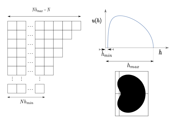
Refer to caption
Figure 15: Young tableaux distribution and density for a generic λ𝜆\lambda. This representation corresponds to a phase space distribution as shown in right bottom figure.

Minimum (hminsubscriptminh_{\text{min}}) and maximum (hmaxsubscriptmaxh_{\text{max}}) values of hh correspond to number of boxes in the last row and first row of Young diagram respectively and are given by

hmax=h+(0)=12+ln2λ+12λln[1+1eλ11eλ],hmin=h(0)=12+ln2λ12λln[1+1eλ11eλ].formulae-sequencesubscriptmaxsubscript0122𝜆12𝜆11superscript𝑒𝜆11superscript𝑒𝜆subscriptminsubscript0122𝜆12𝜆11superscript𝑒𝜆11superscript𝑒𝜆\displaystyle\displaystyle\begin{split}h_{\text{max}}&=h_{+}(0)=\frac{1}{2}+\frac{\ln 2}{\lambda}+\frac{1}{2\lambda}\ln\left[{1+\sqrt{1-e^{-\lambda}}\over 1-\sqrt{1-e^{-\lambda}}}\right],\\ h_{\text{min}}&=h_{-}(0)=\frac{1}{2}+\frac{\ln 2}{\lambda}-\frac{1}{2\lambda}\ln\left[{1+\sqrt{1-e^{-\lambda}}\over 1-\sqrt{1-e^{-\lambda}}}\right].\end{split} (6.28)

For small λ𝜆\lambda, hmaxsubscriptmaxh_{\text{max}} and hminsubscriptminh_{\text{min}} go as

hmaxln2λ+1λ,hminln2λ1λ.formulae-sequencesimilar-tosubscriptmax2𝜆1𝜆similar-tosubscriptmin2𝜆1𝜆h_{\text{max}}\sim\frac{\ln 2}{\lambda}+\frac{1}{\sqrt{\lambda}},\quad h_{\text{min}}\sim\frac{\ln 2}{\lambda}-\frac{1}{\sqrt{\lambda}}. (6.29)

In small λ𝜆\lambda limit we see that both hmaxsubscriptmaxh_{\text{max}} and hminsubscriptminh_{\text{min}} are very large and difference between them goes as 2/λ2𝜆2/\sqrt{\lambda}.

7 Discussion and outlook

In this paper we show that large N𝑁N generic phases of a generic unitary matrix model can be described in terms of geometry of two dimensional droplets in (h,θ)𝜃(h,\theta) plane, where hh is related to number of boxes in Young diagram and θ𝜃\theta is eigenvalue of unitary matrices. We also see that these droplets are similar to phase space distribution of unitary matrix quantum mechanics on a constant time slice. Hence, we argue that for a given unitary matrix model it is possible to find an underlying quantum mechanics such that different large N𝑁N phases of unitary matrix models (and hence interacting gauge theories) are captured on different time slices of the quantum system.

This observation allows us to identify momenta of fermionic system with number of boxes in a Young diagram. Distribution of boxes in Young diagram captures information about the distribution of momenta of N𝑁N fermions. We show that, Young distribution for different large N𝑁N phases can be computed from the geometry of two dimensional droplets. We explicitly work out two examples : β1subscript𝛽1\beta_{1}-β2subscript𝛽2\beta_{2} model and Chern-Simons theory on S3superscript𝑆3S^{3}.

Phase space description of gauge theories can be used to provide a dual quantum mechanical description of string degrees of freedom, since different large N𝑁N phases of gauge theory are dual to classical solutions of string theory in AdS space. Therefore, one can extend this idea for a supersymmetric QFT. One can consider ABJM theory [45], supersymmetric CS theory in 2+1212+1 dimensions. Partition function of ABJM can be calculated exactly for all values of coupling constant. There exists an interpolating function between weak and strong coupling [44, 46]. Hence, it would be interesting to write ABJM partition function in terms of a unitary matrix model and find two dimensional droplets associated with large N𝑁N phases of the theory. One can interpolate this droplet picture to strong coupling side to explore properties/geometries of dual string/M-theories in the spirit of LLM [47]. This will also serve as a precision test of AdS4/CFT3𝐴𝑑subscript𝑆4𝐶𝐹subscript𝑇3AdS_{4}/CFT_{3}. Understanding underlying matrix quantum mechanics for CS theory coupled with matter fields [48, 49, 50, 51, 52] would also be an interesting problem to look at from the point of [53].

One should note that the inviscid Burgers’ equation 4.19 is a generic equation for random matrix theories. In the continuum limit of QCD [54], first observed that spectral density of the Wilson operator follows this equation as a consequence of Makeenko-Migdal equation and proposed a order(gapped)-disorder(gapless) transition for 2D2𝐷2D YM at large N𝑁N. [55] Also came across this same quasi-linear equation while dealing with the continuum version of the loop equation for QCD2𝑄𝐶subscript𝐷2QCD_{2}. Starting with the Burgers’ equation [56, 57] supplemented the proposal of [54], and demonstrated the emergence of a spectral shock wave of Wilson loop eigenvalues at the large Ncsubscript𝑁𝑐N_{c} limit. Recently [58] extended this study numerically for d=4𝑑4d=4. As matrix integrals can be thought of as an alternate way of writing the combinatorics of maps, this kind of connections between random matrix theory and loop equations can also be extended for combinatorial problems. To further explore this combinatorial avenue to understand the identification of loop equations with Tutte’s equations (recursively deleting or contracting edges) and furthermore to grasp the current status of “random matrix” approach to 2D quantum gravity one useful resource would be [59].

On a different ground, UMM has plenty of applications in mathematics specially in number theory. Hilbert and Póyla speculated that there is a spectral origin for non-trivial zeros of Riemann zeta function. It was observed in [60] that if the non-trivial zeros are analogous to EV of some Hamiltonian, then the corresponding conjugate variables, time period of some primitive orbits, are related to prime numbers (proportional to lnp𝑝\ln p where p𝑝p is prime number). Hence, if EV distribution of a UMM captures information about non-trivial zeros, then we expect that corresponding Young distribution function captures information about prime number distribution [11]. It would be nice to understand if there is any quantum mechanical system which captures information about these two distributions.

Acknowledgement

We would like to thank Rajesh Gopakumar for many helpful discussion. We are grateful to Shiraz Minwala and Gautam Mandal for their useful comments on our work. We are grateful to Debashis Ghoshal for innovative discussion. AC would like to acknowledge the hospitality of IISER Pune where part of this work is done. SD acknowledges the Simons Associateship, ICTP. SD also thanks the hospitality of ICTP, Trieste and JNU where part of this work has been done. Work of SD is supported by DST under a project with number EMR/2016/006294. PD is partially supported by research grant number 5304-2, ”Symmetries and Dynamics: Worldsheet and Spacetime” from CEFIPRA/IFCPAR. Finally, we are grateful to people of India for their unconditional support towards researches in basic sciences.

Appendix A Calculation of boundary relation for three trace action

Exponentiating the effective action (3.40) we find,

eSeff=n0exp[an1n2N3TrUn1TrUn2TrU(n1+n2)]exp[an1n2N3TrUn1TrUn2TrU(n1+n2)]=n0[k]=0(an1n2)kn1n2N3kn1n2kn1n2!(TrUn1)kn1n2(TrUn2)kn1n2(TrU(n1+n2))kn1n2[l]=0(an1n2)ln1n2N3ln1n2ln1n2!(TrUn1)ln1n2(TrUn2)ln1n2(TrU(n1+n2))ln1n2formulae-sequencesuperscript𝑒subscript𝑆𝑒𝑓𝑓subscriptproduct𝑛0subscript𝑎subscript𝑛1subscript𝑛2superscript𝑁3Trsuperscript𝑈subscript𝑛1Trsuperscript𝑈subscript𝑛2Trsuperscript𝑈absentsubscript𝑛1subscript𝑛2subscript𝑎subscript𝑛1subscript𝑛2superscript𝑁3Trsuperscript𝑈absentsubscript𝑛1Trsuperscript𝑈absentsubscript𝑛2Trsuperscript𝑈subscript𝑛1subscript𝑛2subscriptproduct𝑛0superscriptsubscriptdelimited-[]𝑘0superscriptsubscript𝑎subscript𝑛1subscript𝑛2subscript𝑘subscript𝑛1subscript𝑛2superscript𝑁3subscript𝑘subscript𝑛1subscript𝑛2subscript𝑘subscript𝑛1subscript𝑛2superscriptTrsuperscript𝑈subscript𝑛1subscript𝑘subscript𝑛1subscript𝑛2superscriptTrsuperscript𝑈subscript𝑛2subscript𝑘subscript𝑛1subscript𝑛2superscriptTrsuperscript𝑈absentsubscript𝑛1subscript𝑛2subscript𝑘subscript𝑛1subscript𝑛2superscriptsubscriptdelimited-[]𝑙0superscriptsubscript𝑎subscript𝑛1subscript𝑛2subscript𝑙subscript𝑛1subscript𝑛2superscript𝑁3subscript𝑙subscript𝑛1subscript𝑛2subscript𝑙subscript𝑛1subscript𝑛2superscriptTrsuperscript𝑈absentsubscript𝑛1subscript𝑙subscript𝑛1subscript𝑛2superscriptTrsuperscript𝑈absentsubscript𝑛2subscript𝑙subscript𝑛1subscript𝑛2superscriptTrsuperscript𝑈subscript𝑛1subscript𝑛2subscript𝑙subscript𝑛1subscript𝑛2\displaystyle\begin{split}e^{S_{eff}}&=\prod_{\vec{n}\geq 0}\exp\left[{a_{n_{1}n_{2}}\over N^{3}}\text{Tr}{U^{n_{1}}}\text{Tr}{U^{n_{2}}}\text{Tr}{U^{\dagger(n_{1}+n_{2})}}\right]\exp\left[{a_{n_{1}n_{2}}\over N^{3}}\text{Tr}{U^{\dagger n_{1}}}\text{Tr}{U^{\dagger n_{2}}}\text{Tr}{U^{(n_{1}+n_{2})}}\right]\\ &=\prod_{\vec{n}\geq 0}\sum_{[k]=0}^{\infty}{(a_{n_{1}n_{2}})^{k_{n_{1}n_{2}}}\over N^{3k_{n_{1}n_{2}}}k_{n_{1}n_{2}!}}(\text{Tr}{U^{n_{1}}})^{k_{n_{1}n_{2}}}(\text{Tr}{U^{n_{2}}})^{k_{n_{1}n_{2}}}(\text{Tr}{U^{\dagger(n_{1}+n_{2})}})^{k_{n_{1}n_{2}}}\\ &\qquad\quad\sum_{[l]=0}^{\infty}{(a_{n_{1}n_{2}})^{l_{n_{1}n_{2}}}\over N^{3l_{n_{1}n_{2}}}l_{n_{1}n_{2}!}}(\text{Tr}{U^{\dagger n_{1}}})^{l_{n_{1}n_{2}}}(\text{Tr}{U^{\dagger n_{2}}})^{l_{n_{1}n_{2}}}(\text{Tr}{U^{(n_{1}+n_{2})}})^{l_{n_{1}n_{2}}}\end{split} (A.1)

where, n𝑛\vec{n} is a two dimensional vector with entries n1subscript𝑛1n_{1} and n2subscript𝑛2n_{2}, [k]delimited-[]𝑘[k] and [l]delimited-[]𝑙[l] are matrices with entries kn1n2subscript𝑘subscript𝑛1subscript𝑛2k_{n_{1}n_{2}} and ln1n2subscript𝑙subscript𝑛1subscript𝑛2l_{n_{1}n_{2}}. Interchanging the sum and product we write

eSeff=[k],[l]n0(an1n2)kn1n2+ln1n2kn1n2!ln1n2!n0(TrUn1)kn1n2(TrUn2)kn1n2(TrUn1+n2)kn1n2n0(TrUn1)ln1n2(TrUn2)ln1n2(TrUn1+n2)ln1n2.superscript𝑒subscript𝑆𝑒𝑓𝑓subscriptdelimited-[]𝑘delimited-[]𝑙subscriptproduct𝑛0superscriptsubscript𝑎subscript𝑛1subscript𝑛2subscript𝑘subscript𝑛1subscript𝑛2subscript𝑙subscript𝑛1subscript𝑛2subscript𝑘subscript𝑛1subscript𝑛2subscript𝑙subscript𝑛1subscript𝑛2subscriptproduct𝑛0superscriptTrsuperscript𝑈subscript𝑛1subscript𝑘subscript𝑛1subscript𝑛2superscriptTrsuperscript𝑈subscript𝑛2subscript𝑘subscript𝑛1subscript𝑛2superscriptTrsuperscript𝑈absentsubscript𝑛1subscript𝑛2subscript𝑘subscript𝑛1subscript𝑛2subscriptproduct𝑛0superscriptTrsuperscript𝑈absentsubscript𝑛1subscript𝑙subscript𝑛1subscript𝑛2superscriptTrsuperscript𝑈absentsubscript𝑛2subscript𝑙subscript𝑛1subscript𝑛2superscriptTrsuperscript𝑈subscript𝑛1subscript𝑛2subscript𝑙subscript𝑛1subscript𝑛2\displaystyle\displaystyle\begin{split}e^{S_{eff}}&=\sum_{[k],[l]}\prod_{\vec{n}\geq 0}{(a_{n_{1}n_{2}})^{k_{n_{1}n_{2}}+l_{n_{1}n_{2}}}\over k_{n_{1}n_{2}}!l_{n_{1}n_{2}}!}\\ &\qquad\prod_{\vec{n}\geq 0}\left(\text{Tr}U^{{n_{1}}}\right)^{k_{n_{1}n_{2}}}\left(\text{Tr}U^{{n_{2}}}\right)^{k_{n_{1}n_{2}}}\left(\text{Tr}U^{\dagger{n_{1}+n_{2}}}\right)^{k_{n_{1}n_{2}}}\\ &\qquad\prod_{\vec{n}\geq 0}\left(\text{Tr}U^{\dagger{n_{1}}}\right)^{l_{n_{1}n_{2}}}\left(\text{Tr}U^{\dagger{n_{2}}}\right)^{l_{n_{1}n_{2}}}\left(\text{Tr}U^{{n_{1}+n_{2}}}\right)^{l_{n_{1}n_{2}}}.\end{split} (A.2)

This expression can be further simplified to,

eSeff=[k],[l]𝒯0Np0+q0+r0+s0Υp+r(U)Υq+s(U)superscript𝑒subscript𝑆𝑒𝑓𝑓subscriptdelimited-[]𝑘delimited-[]𝑙subscript𝒯0superscript𝑁subscript𝑝0subscript𝑞0subscript𝑟0subscript𝑠0subscriptΥ𝑝𝑟𝑈subscriptΥ𝑞𝑠superscript𝑈\displaystyle\displaystyle\begin{split}e^{S_{eff}}&=\sum_{[k],[l]}\mathcal{T}_{0}\ N^{p_{0}+q_{0}+r_{0}+s_{0}}\Upsilon_{\vec{p}+\vec{r}}(U)\Upsilon_{\vec{q}+\vec{s}}(U^{\dagger{}})\end{split} (A.3)

where,

pi=j=0kij+kji,qi=m,m=0kmnδ(m+ni)i=0,1,2,si=j=0lij+lji,ri=m,n=0lmnδ(m+ni)i=0,1,2,,\displaystyle\displaystyle\begin{split}p_{i}&=\sum_{j=0}^{\infty}k_{ij}+k_{ji},\quad q_{i}=\sum_{m,m=0}^{\infty}k_{mn}\delta(m+n-i)\quad\forall\ i=0,1,2,\cdots\\ s_{i}&=\sum_{j=0}^{\infty}l_{ij}+l_{ji},\quad r_{i}=\sum_{m,n=0}l_{mn}\,\delta(m+n-i)\quad\forall\ i=0,1,2,\cdots,\end{split} (A.4)

p={p1,p2,}𝑝subscript𝑝1subscript𝑝2\vec{p}=\{p_{1},p_{2},\cdots\}, q={q1,q2,}𝑞subscript𝑞1subscript𝑞2\vec{q}=\{q_{1},q_{2},\cdots\}, r={r1,r2,}𝑟subscript𝑟1subscript𝑟2\vec{r}=\{r_{1},r_{2},\cdots\}, s={s1,s2,}𝑠subscript𝑠1subscript𝑠2\vec{s}=\{s_{1},s_{2},\cdots\} and

Υp+r(U)=n=1(TrUn)pn+rn.subscriptΥ𝑝𝑟𝑈superscriptsubscriptproduct𝑛1superscriptTrsuperscript𝑈𝑛subscript𝑝𝑛subscript𝑟𝑛\Upsilon_{\vec{p}+\vec{r}}(U)=\prod_{n=1}^{\infty}\left(\text{Tr}U^{{n}}\right)^{p_{n}+r_{n}}. (A.5)

The partition function, therefore, is given by,

𝒵𝒵\displaystyle\mathcal{Z} =\displaystyle= [DU][k][l]𝒯0Nq0+p0+r0+s0Υp+r(U)Υq+s(U).delimited-[]𝐷𝑈subscriptdelimited-[]𝑘subscriptdelimited-[]𝑙subscript𝒯0superscript𝑁subscript𝑞0subscript𝑝0subscript𝑟0subscript𝑠0subscriptΥ𝑝𝑟𝑈subscriptΥ𝑞𝑠superscript𝑈\displaystyle\int[DU]\sum_{[k]}\sum_{[l]}\,\mathcal{T}_{0}\,\,N^{q_{0}+p_{0}+r_{0}+s_{0}}\,\,\Upsilon_{\vec{p}+\vec{r}}(U)\Upsilon_{\vec{q}+\vec{s}}(U^{\dagger}). (A.6)

ΥΥ\Upsilon’s can be written, like before, in terms of the characters of the permutation group using the following identity

Υp+r(U)subscriptΥ𝑝𝑟𝑈\displaystyle\Upsilon_{\vec{p}+\vec{r}}(U) =\displaystyle= RχR(C(p+r))TrRUsubscript𝑅subscript𝜒𝑅𝐶𝑝𝑟subscriptTr𝑅𝑈\displaystyle\sum_{R}\chi_{R}(C(\vec{p}+\vec{r}))\text{Tr}_{R}U (A.7)
Υq+s(U)subscriptΥ𝑞𝑠𝑈\displaystyle\Upsilon_{\vec{q}+\vec{s}}(U) =\displaystyle= RχR(C(q+s))TrRUsubscriptsuperscript𝑅subscript𝜒superscript𝑅𝐶𝑞𝑠subscriptTrsuperscript𝑅superscript𝑈\displaystyle\sum_{R^{{}^{\prime}}}\chi_{R^{{}^{\prime}}}(C(\vec{q}+\vec{s}))\text{Tr}_{R^{{}^{\prime}}}U^{\dagger{}} (A.8)

Substituting ΥΥ\Upsilon in equation (A.6) and using orthogonality relation (3.5) we find,

𝒵=R[k][l]𝒯0χR(c(p+r))χR(c(q+s)).𝒵subscript𝑅subscriptdelimited-[]𝑘subscriptdelimited-[]𝑙subscript𝒯0subscript𝜒𝑅𝑐𝑝𝑟subscript𝜒𝑅𝑐𝑞𝑠\displaystyle\mathcal{Z}=\sum_{R}\sum_{[k]}\sum_{[l]}\,\mathcal{T}_{0}\,\,\chi_{R}(c(\vec{p}+\vec{r}))\chi_{R}(c(\vec{q}+\vec{s})). (A.9)

One can write sum of representations of U(N)𝑈𝑁U(N) as sum over different Young diagrams. Finally, partition function is given by,

𝒵={λα}[k][l]𝒯0χR(C(p+r))χR(C(q+s))δ(Σii(pi+ri)Σαλα)δ(Σii(qi+si)Σαλα).𝒵subscriptsubscript𝜆𝛼subscriptdelimited-[]𝑘delimited-[]𝑙subscript𝒯0subscript𝜒𝑅𝐶𝑝𝑟subscript𝜒𝑅𝐶𝑞𝑠𝛿subscriptΣ𝑖𝑖subscript𝑝𝑖subscript𝑟𝑖subscriptΣ𝛼subscript𝜆𝛼𝛿subscriptΣ𝑖𝑖subscript𝑞𝑖subscript𝑠𝑖subscriptΣ𝛼subscript𝜆𝛼\displaystyle\displaystyle\mathcal{Z}=\sum_{\{\lambda_{\alpha}\}}\sum_{[k][l]}\mathcal{T}_{0}\ \chi_{R}(C(\vec{p}+\vec{r}))\chi_{R}(C(\vec{q}+\vec{s}))\delta(\Sigma_{i}i(p_{i}+r_{i})-\Sigma_{\alpha}\lambda_{\alpha})\delta(\Sigma_{i}i(q_{i}+s_{i})-\Sigma_{\alpha}\lambda_{\alpha}).

A.1 Extremization of partition function

In large N𝑁N limit we define,

an1n2=N2an1n2;kn1n2=N2kn1n2;ln1n2=N2ln1n2;K=N2Kformulae-sequencesubscript𝑎subscript𝑛1subscript𝑛2superscript𝑁2superscriptsubscript𝑎subscript𝑛1subscript𝑛2formulae-sequencesubscript𝑘subscript𝑛1subscript𝑛2superscript𝑁2superscriptsubscript𝑘subscript𝑛1subscript𝑛2formulae-sequencesubscript𝑙subscript𝑛1subscript𝑛2superscript𝑁2superscriptsubscript𝑙subscript𝑛1subscript𝑛2𝐾superscript𝑁2superscript𝐾a_{n_{1}n_{2}}=N^{2}a_{n_{1}n_{2}}^{{}^{\prime}};\quad k_{n_{1}n_{2}}=N^{2}k_{n_{1}n_{2}}^{{}^{\prime}};\quad l_{n_{1}n_{2}}=N^{2}l_{n_{1}n_{2}}^{{}^{\prime}};\quad K=N^{2}K^{\prime} (A.11)

and using the expression for character given by equation (3.22), partition function (A) can be written as, (see next subsection A.2 for details)

𝒵𝒵\displaystyle\mathcal{Z} =\displaystyle= N4(2πi)2Nd[k]d[l][Dh][Dz]z(x)[Dw]w(x)𝑑t𝑑sexp[N2Seff(h,z,w)]superscript𝑁4superscript2𝜋𝑖2𝑁𝑑delimited-[]superscript𝑘𝑑delimited-[]superscript𝑙delimited-[]𝐷delimited-[]𝐷𝑧𝑧𝑥delimited-[]𝐷𝑤𝑤𝑥differential-d𝑡differential-d𝑠superscript𝑁2subscript𝑆eff𝑧𝑤\displaystyle{N^{4}\over(2\pi i)^{2N}}\int d[k^{\prime}]d[l^{\prime}]\int[Dh]{[Dz]\over z(x)}{[Dw]\over w(x)}\int dt\,ds\exp\left[-N^{2}S_{\text{eff}}({h,z,w})\right] (A.12)

where,

d[k]=n1,n2=0dkn1n2,d[l]=n1,n2=0dln1n2formulae-sequence𝑑delimited-[]superscript𝑘subscriptproductsubscript𝑛1subscript𝑛20𝑑subscriptsuperscript𝑘subscript𝑛1subscript𝑛2𝑑delimited-[]superscript𝑙subscriptproductsubscript𝑛1subscript𝑛20𝑑subscriptsuperscript𝑙subscript𝑛1subscript𝑛2\qquad d[k^{\prime}]=\prod_{n_{1},n_{2}=0}dk^{\prime}_{n_{1}n_{2}},\quad d[l^{\prime}]=\prod_{n_{1},n_{2}=0}dl^{\prime}_{n_{1}n_{2}}

and

Seff(h,z,w)subscript𝑆eff𝑧𝑤\displaystyle-S_{\text{eff}}({h,z,w}) =\displaystyle= n1,n2=0[kn1n2(1+ln(an1n2Zn1Zn2Wn1+n2kn1n2))\displaystyle\sum_{n_{1},n_{2}=0}^{\infty}\Bigg{[}k_{n_{1}n_{2}}^{\prime}\left(1+\ln\left(a_{n_{1}n_{2}}^{\prime}Z_{n_{1}}Z_{n_{2}}W_{n_{1}+n_{2}}\over k_{n_{1}n_{2}}^{\prime}\right)\right) (A.13)
+ln1n2(1+ln(an1n2Wn1Wn2Zn1+n2ln1n2))]\displaystyle+l_{n_{1}n_{2}}^{\prime}\left(1+\ln\left(a_{n_{1}n_{2}}^{\prime}W_{n_{1}}W_{n_{2}}Z_{n_{1}+n_{2}}\over l_{n_{1}n_{2}}^{\prime}\right)\right)\Bigg{]}
01𝑑xh(x)ln(z(x)w(x))+1201𝑑x01𝑑yln(|z(x)z(y)||w(x)w(y)|)superscriptsubscript01differential-d𝑥𝑥𝑧𝑥𝑤𝑥12superscriptsubscript01differential-d𝑥superscriptsubscript01differential-d𝑦𝑧𝑥𝑧𝑦𝑤𝑥𝑤𝑦\displaystyle-\int_{0}^{1}dx\,h(x)\,\ln\left(z(x)w(x)\right)+\frac{1}{2}\int_{0}^{1}dx\mathchoice{{\vbox{\hbox{$\textstyle-$ }}\kern-7.83337pt}}{{\vbox{\hbox{$\scriptstyle-$ }}\kern-5.90005pt}}{{\vbox{\hbox{$\scriptscriptstyle-$ }}\kern-4.75003pt}}{{\vbox{\hbox{$\scriptscriptstyle-$ }}\kern-4.25003pt}}\!\int_{0}^{1}dy\,\ln\left(|z(x)-z(y)||w(x)-w(y)|\right)
+i(t+s)(n1,n2=0(n1+n2)(kn1n2+ln1n2)K)𝑖𝑡𝑠superscriptsubscriptsubscript𝑛1subscript𝑛20subscript𝑛1subscript𝑛2superscriptsubscript𝑘subscript𝑛1subscript𝑛2superscriptsubscript𝑙subscript𝑛1subscript𝑛2superscript𝐾\displaystyle+i(t+s)(\sum_{n_{1},n_{2}=0}^{\infty}(n_{1}+n_{2})(k_{n_{1}n_{2}}^{\prime}+l_{n_{1}n_{2}}^{\prime})-K^{\prime})

where,

Zn=zn(x)𝑑xandWn=wn(x)𝑑x.formulae-sequencesubscript𝑍𝑛superscript𝑧𝑛𝑥differential-d𝑥andsubscript𝑊𝑛superscript𝑤𝑛𝑥differential-d𝑥Z_{n}=\int z^{n}(x)dx\quad\text{and}\quad W_{n}=\int w^{n}(x)dx. (A.14)

In the large N𝑁N limit dominant contribution to partition function comes from extremum value of this effective action. Varying this effective action with respect to h(x)𝑥h(x) we find,

z(x)w(x)=ei(t+s)=constant.𝑧𝑥𝑤𝑥superscript𝑒𝑖𝑡𝑠constant\displaystyle z(x)w(x)=e^{-i(t+s)}=\text{constant}. (A.15)

Again, varying the effective action with respect to kn1n2superscriptsubscript𝑘subscript𝑛1subscript𝑛2k_{n_{1}n_{2}}^{\prime} and ln1n2superscriptsubscript𝑙subscript𝑛1subscript𝑛2l_{n_{1}n_{2}}^{\prime} one can write

an1n2Zn1Zn2Wn1+n2kn1n2=ei(t+s)(n1+n2)=constant,an1n2Wn1Wn2Zn1+n2ln1n2=ei(t+s)(n1+n2)=constant.formulae-sequencesuperscriptsubscript𝑎subscript𝑛1subscript𝑛2subscript𝑍subscript𝑛1subscript𝑍subscript𝑛2subscript𝑊subscript𝑛1subscript𝑛2superscriptsubscript𝑘subscript𝑛1subscript𝑛2superscript𝑒𝑖𝑡𝑠subscript𝑛1subscript𝑛2constantsuperscriptsubscript𝑎subscript𝑛1subscript𝑛2subscript𝑊subscript𝑛1subscript𝑊subscript𝑛2subscript𝑍subscript𝑛1subscript𝑛2superscriptsubscript𝑙subscript𝑛1subscript𝑛2superscript𝑒𝑖𝑡𝑠subscript𝑛1subscript𝑛2constant\displaystyle\begin{split}{a_{n_{1}n_{2}}^{\prime}Z_{n_{1}}Z_{n_{2}}W_{n_{1}+n_{2}}\over k_{n_{1}n_{2}}^{\prime}}&=e^{-i(t+s)(n_{1}+n_{2})}=\text{constant},\\ {a_{n_{1}n_{2}}^{\prime}W_{n_{1}}W_{n_{2}}Z_{n_{1}+n_{2}}\over l_{n_{1}n_{2}}^{\prime}}&=e^{-i(t+s)(n_{1}+n_{2})}=\text{constant}.\end{split} (A.16)

Finally, varying Seff(h,z,w)subscript𝑆eff𝑧𝑤S_{\text{eff}}({h,z,w}) with respect to z(x)𝑧𝑥z(x) we find,

01𝑑yz(x)z(x)z(y)h(x)+n1n2=0[kn1n2(n1zn1(x)Zn1+n2zn2(x)Zn2)+ln1n2(n1+n2)zn1+n2(x)Zn1+n2]=0.superscriptsubscript01differential-d𝑦𝑧𝑥𝑧𝑥𝑧𝑦𝑥superscriptsubscriptsubscript𝑛1subscript𝑛20delimited-[]superscriptsubscript𝑘subscript𝑛1subscript𝑛2subscript𝑛1superscript𝑧subscript𝑛1𝑥subscript𝑍subscript𝑛1subscript𝑛2superscript𝑧subscript𝑛2𝑥subscript𝑍subscript𝑛2superscriptsubscript𝑙subscript𝑛1subscript𝑛2subscript𝑛1subscript𝑛2superscript𝑧subscript𝑛1subscript𝑛2𝑥subscript𝑍subscript𝑛1subscript𝑛20\displaystyle\mathchoice{{\vbox{\hbox{$\textstyle-$ }}\kern-7.83337pt}}{{\vbox{\hbox{$\scriptstyle-$ }}\kern-5.90005pt}}{{\vbox{\hbox{$\scriptscriptstyle-$ }}\kern-4.75003pt}}{{\vbox{\hbox{$\scriptscriptstyle-$ }}\kern-4.25003pt}}\!\int_{0}^{1}dy\,{z(x)\over z(x)-z(y)}-h(x)+\sum_{n_{1}n_{2}=0}^{\infty}\Bigg{[}k_{n_{1}n_{2}}^{\prime}\left({n_{1}z^{n_{1}}(x)\over Z_{n_{1}}}+{n_{2}z^{n_{2}}(x)\over Z_{n_{2}}}\right)+l_{n_{1}n_{2}}^{\prime}{(n_{1}+n_{2})z^{n_{1}+n_{2}}(x)\over Z_{n_{1}+n_{2}}}\Bigg{]}=0.

A similar equation can be obtained when we vary the effective with respective to w(x)𝑤𝑥w(x) with z(x)𝑧𝑥z(x) replaced by w(x)𝑤𝑥w(x).

Since, in equation (A.12) z(x)𝑧𝑥z(x) and w(x)𝑤𝑥w(x) vary over some contour around zero, we take these contours to be unit circle about the origin and hence one consistent set of solutions to equations (A.15) and (A.16) are given by,

z(x)=eiθ(x),w(x)=eθ(x),t=s=0.formulae-sequence𝑧𝑥superscript𝑒𝑖𝜃𝑥formulae-sequence𝑤𝑥superscript𝑒𝜃𝑥𝑡𝑠0\displaystyle\displaystyle z(x)=e^{i\theta(x)},\quad w(x)=e^{-\theta(x)},\quad t=s=0. (A.18)

Therefore,

Zn=Wn(for alln)andkn1n2=ln1n2=an1n2Zn1Zn2Zn1+n2.formulae-sequencesubscript𝑍𝑛subscript𝑊𝑛for all𝑛andsubscriptsuperscript𝑘subscript𝑛1subscript𝑛2subscriptsuperscript𝑙subscript𝑛1subscript𝑛2subscriptsuperscript𝑎subscript𝑛1subscript𝑛2subscript𝑍subscript𝑛1subscript𝑍subscript𝑛2subscript𝑍subscript𝑛1subscript𝑛2\displaystyle\displaystyle Z_{n}=W_{n}\quad(\text{for all}\ n)\quad\text{and}\quad k^{\prime}_{n_{1}n_{2}}=l^{\prime}_{n_{1}n_{2}}=a^{\prime}_{n_{1}n_{2}}Z_{n_{1}}Z_{n_{2}}Z_{n_{1}+n_{2}}. (A.19)

Using these solutions the saddle point equation for z(x)=exp(iθ(x))𝑧𝑥𝑖𝜃𝑥z(x)=\exp(i\theta(x)) is given by equation (3.2).

A.2 Details of partition function calculation

We have

𝒵𝒵\displaystyle\mathcal{Z} =\displaystyle= n1,n2=0N4(2πi)2Ndkn1n2dln1n2[Dh][Dz]z(x)[Dw]w(x)dtdsexpN2(n1,n2=0[(kn1n2+ln1n2)ln(an1n2N)\displaystyle\prod_{n_{1},n_{2}=0}{N^{4}\over(2\pi i)^{2N}}\int\begin{matrix}&dk_{n_{1}n_{2}}^{{}^{\prime}}\\ &dl_{n_{1}n_{2}}^{{}^{\prime}}\end{matrix}\int[Dh]{[Dz]\over z(x)}{[Dw]\over w(x)}\int dt\,ds\,\exp N^{2}\Bigg{(}\sum_{n_{1},n_{2}=0}\Big{[}(k_{n_{1}n_{2}}^{{}^{\prime}}+l_{n_{1}n_{2}}^{{}^{\prime}})\ln\left(a_{n_{1}n_{2}}^{{}^{\prime}}\over N\right) (A.20)
2kn1n2ln(N)kn1n2ln(kn1n2)+kn1n22ln1n2ln(N)ln1n2ln(ln1n2)+ln1n2]\displaystyle-2k_{n_{1}n_{2}}^{\prime}\ln\left(N\right)-k_{n_{1}n_{2}}^{\prime}\ln\left(k_{n_{1}n_{2}}^{\prime}\right)+k_{n_{1}n_{2}}^{\prime}-2l_{n_{1}n_{2}}^{\prime}\ln\left(N\right)-l_{n_{1}n_{2}}^{\prime}\ln\left(l_{n_{1}n_{2}}^{\prime}\right)+l_{n_{1}n_{2}}^{\prime}\Big{]}
+(k00+l00+p0+q0)ln(N)+it(jj(pj+rj)K)+is(jj(qj+sj)K)superscriptsubscript𝑘00superscriptsubscript𝑙00superscriptsubscript𝑝0superscriptsubscript𝑞0𝑁𝑖𝑡subscript𝑗𝑗superscriptsubscript𝑝𝑗superscriptsubscript𝑟𝑗superscript𝐾𝑖𝑠subscript𝑗𝑗superscriptsubscript𝑞𝑗superscriptsubscript𝑠𝑗superscript𝐾\displaystyle+(k_{00}^{\prime}+l_{00}^{\prime}+p_{0}^{\prime}+q_{0}^{\prime})\ln\left(N\right)+it(\sum_{j}j(p_{j}^{\prime}+r_{j}^{\prime})-K^{\prime})+is(\sum_{j}j(q_{j}^{\prime}+s_{j}^{\prime})-K^{\prime})
+n=1(pn+rn)ln(NZn)+n=1(qn+sn)ln(NWn)+1201𝑑x01𝑑yln(|z(x)z(y)||w(x)w(y)|)superscriptsubscript𝑛1superscriptsubscript𝑝𝑛superscriptsubscript𝑟𝑛𝑁subscript𝑍𝑛superscriptsubscript𝑛1superscriptsubscript𝑞𝑛superscriptsubscript𝑠𝑛𝑁subscript𝑊𝑛12superscriptsubscript01differential-d𝑥superscriptsubscript01differential-d𝑦𝑧𝑥𝑧𝑦𝑤𝑥𝑤𝑦\displaystyle+\sum_{n=1}^{\infty}(p_{n}^{\prime}+r_{n}^{\prime})\ln\left(NZ_{n}\right)+\sum_{n=1}^{\infty}(q_{n}^{\prime}+s_{n}^{\prime})\ln\left(NW_{n}\right)+\frac{1}{2}\int_{0}^{1}dx\mathchoice{{\vbox{\hbox{$\textstyle-$ }}\kern-7.83337pt}}{{\vbox{\hbox{$\scriptstyle-$ }}\kern-5.90005pt}}{{\vbox{\hbox{$\scriptscriptstyle-$ }}\kern-4.75003pt}}{{\vbox{\hbox{$\scriptscriptstyle-$ }}\kern-4.25003pt}}\!\int_{0}^{1}dy\,\ln\left(|z(x)-z(y)||w(x)-w(y)|\right)
01dxh(x)ln(z(x)w(x))).\displaystyle-\int_{0}^{1}dx\,h(x)\,\ln\left(z(x)w(x)\right)\Bigg{)}.

Now let us look into some relations

n=1pnln(NZn)superscriptsubscript𝑛1superscriptsubscript𝑝𝑛𝑁subscript𝑍𝑛\displaystyle\sum_{n=1}^{\infty}p_{n}^{\prime}\ln\left(NZ_{n}\right) =\displaystyle= n=0pnln(NZn)p0ln(NZn)superscriptsubscript𝑛0superscriptsubscript𝑝𝑛𝑁subscript𝑍𝑛superscriptsubscript𝑝0𝑁subscript𝑍𝑛\displaystyle\sum_{n=0}^{\infty}p_{n}^{\prime}\ln\left(NZ_{n}\right)-p_{0}^{\prime}\ln\left(NZ_{n}\right) (A.21)
=\displaystyle= n1=0n2=0(kn1n2+kn2n1)ln(NZn1)p0ln(NZ0)superscriptsubscriptsubscript𝑛10superscriptsubscriptsubscript𝑛20superscriptsubscript𝑘subscript𝑛1subscript𝑛2superscriptsubscript𝑘subscript𝑛2subscript𝑛1𝑁subscript𝑍subscript𝑛1superscriptsubscript𝑝0𝑁subscript𝑍0\displaystyle\sum_{n_{1}=0}^{\infty}\sum_{n_{2}=0}^{\infty}(k_{n_{1}n_{2}}^{\prime}+k_{n_{2}n_{1}}^{\prime})\ln\left(NZ_{n_{1}}\right)-p_{0}^{\prime}\ln\left(NZ_{0}\right)
=\displaystyle= n1,n2=0kn1n2ln(N2Zn1Zn2)p0ln(N)superscriptsubscriptsubscript𝑛1subscript𝑛20superscriptsubscript𝑘subscript𝑛1subscript𝑛2superscript𝑁2subscript𝑍subscript𝑛1subscript𝑍subscript𝑛2superscriptsubscript𝑝0𝑁\displaystyle\sum_{n_{1},n_{2}=0}^{\infty}k_{n_{1}n_{2}}^{\prime}\ln\left(N^{2}Z_{n_{1}}Z_{n_{2}}\right)-p_{0}^{\prime}\ln\left(N\right)
n1=0n2=0m=0ln2mδ(m+n2n1)superscriptsubscriptsubscript𝑛10superscriptsubscriptsubscript𝑛20superscriptsubscript𝑚0superscriptsubscript𝑙subscript𝑛2𝑚𝛿𝑚subscript𝑛2subscript𝑛1\displaystyle\sum_{n_{1}=0}^{\infty}\sum_{n_{2}=0}^{\infty}\sum_{m=0}^{\infty}l_{n_{2}m}^{\prime}\delta(m+n_{2}-n_{1}) =\displaystyle= l00+(l01+l10)+(l02+l11+l20)+superscriptsubscript𝑙00superscriptsubscript𝑙01superscriptsubscript𝑙10superscriptsubscript𝑙02superscriptsubscript𝑙11subscript𝑙20\displaystyle l_{00}^{\prime}+(l_{01}^{\prime}+l_{10}^{\prime})+(l_{02}^{\prime}+l_{11}^{\prime}+l_{20})+\cdots (A.22)
=\displaystyle= l00+(l01+l02+)+(l10+l11+l12+)+superscriptsubscript𝑙00superscriptsubscript𝑙01superscriptsubscript𝑙02superscriptsubscript𝑙10superscriptsubscript𝑙11superscriptsubscript𝑙12\displaystyle l_{00}^{\prime}+(l_{01}^{\prime}+l_{02}^{\prime}+\cdots)+(l_{10}^{\prime}+l_{11}^{\prime}+l_{12}^{\prime}+\cdots)+\cdots
=\displaystyle= n1,n2=0ln1n2superscriptsubscriptsubscript𝑛1subscript𝑛20subscript𝑙subscript𝑛1subscript𝑛2\displaystyle\sum_{n_{1},n_{2}=0}^{\infty}l_{n_{1}n_{2}}
n=1rnln(NZn)superscriptsubscript𝑛1superscriptsubscript𝑟𝑛𝑁subscript𝑍𝑛\displaystyle\sum_{n=1}^{\infty}r_{n}^{\prime}\ln\left(NZ_{n}\right) =\displaystyle= n=0rnln(NZn)r0ln(NZn)superscriptsubscript𝑛0superscriptsubscript𝑟𝑛𝑁subscript𝑍𝑛superscriptsubscript𝑟0𝑁subscript𝑍𝑛\displaystyle\sum_{n=0}^{\infty}r_{n}^{\prime}\ln\left(NZ_{n}\right)-r_{0}^{\prime}\ln\left(NZ_{n}\right) (A.23)
=\displaystyle= n1=0n2=0m=0ln2mδ(m+n2n1)ln(NZn1)r0ln(NZ0)superscriptsubscriptsubscript𝑛10superscriptsubscriptsubscript𝑛20superscriptsubscript𝑚0superscriptsubscript𝑙subscript𝑛2𝑚𝛿𝑚subscript𝑛2subscript𝑛1𝑁subscript𝑍subscript𝑛1superscriptsubscript𝑟0𝑁subscript𝑍0\displaystyle\sum_{n_{1}=0}^{\infty}\sum_{n_{2}=0}^{\infty}\sum_{m=0}^{\infty}l_{n_{2}m}^{\prime}\delta(m+n_{2}-n_{1})\ln\left(NZ_{n_{1}}\right)-r_{0}^{\prime}\ln\left(NZ_{0}\right)
=\displaystyle= n1,n2=0ln1n2ln(NZn1+n2)r0ln(N)superscriptsubscriptsubscript𝑛1subscript𝑛20superscriptsubscript𝑙subscript𝑛1subscript𝑛2𝑁subscript𝑍subscript𝑛1subscript𝑛2superscriptsubscript𝑟0𝑁\displaystyle\sum_{n_{1},n_{2}=0}^{\infty}l_{n_{1}n_{2}}^{\prime}\ln\left(NZ_{n_{1}+n_{2}}\right)-r_{0}^{\prime}\ln\left(N\right)

So finally we have the partition function as

𝒵𝒵\displaystyle\mathcal{Z} =\displaystyle= n1,n2=0N4(2πi)2Ndkn1n2dtdln1n2ds[Dh][Dz]z(x)[Dw]w(x)expN2[it(j=1j(pj+rj)K)+is(j=1j(qj+sj)K)\displaystyle\prod_{n_{1},n_{2}=0}{N^{4}\over(2\pi i)^{2N}}\int\begin{matrix}&dk_{n_{1}n_{2}}^{{}^{\prime}}\,dt\\ &dl_{n_{1}n_{2}}^{{}^{\prime}}\,ds\end{matrix}\int[Dh]\int\,{[Dz]\over z(x)}{[Dw]\over w(x)}\,\exp N^{2}\Bigg{[}\begin{matrix}&it(\sum_{j=1}^{\infty}j(p_{j}^{\prime}+r_{j}^{\prime})-K^{\prime})\\ &+is(\sum_{j=1}^{\infty}j(q_{j}^{\prime}+s_{j}^{\prime})-K^{\prime})\end{matrix} (A.24)
+n1,n2=0(kn1n2(1+ln(an1n2Zn1Zn2Wn1+n2kn1n2))+ln1n2(1+ln(an1n2Wn1Wn2Zn1+n2ln1n2)))superscriptsubscriptsubscript𝑛1subscript𝑛20superscriptsubscript𝑘subscript𝑛1subscript𝑛21superscriptsubscript𝑎subscript𝑛1subscript𝑛2subscript𝑍subscript𝑛1subscript𝑍subscript𝑛2subscript𝑊subscript𝑛1subscript𝑛2superscriptsubscript𝑘subscript𝑛1subscript𝑛2superscriptsubscript𝑙subscript𝑛1subscript𝑛21superscriptsubscript𝑎subscript𝑛1subscript𝑛2subscript𝑊subscript𝑛1subscript𝑊subscript𝑛2subscript𝑍subscript𝑛1subscript𝑛2superscriptsubscript𝑙subscript𝑛1subscript𝑛2\displaystyle+\sum_{n_{1},n_{2}=0}^{\infty}\Bigg{(}k_{n_{1}n_{2}}^{\prime}(1+\ln\left(a_{n_{1}n_{2}}^{\prime}Z_{n_{1}}Z_{n_{2}}W_{n_{1}+n_{2}}\over k_{n_{1}n_{2}}^{\prime}\right))+l_{n_{1}n_{2}}^{\prime}(1+\ln\left(a_{n_{1}n_{2}}^{\prime}W_{n_{1}}W_{n_{2}}Z_{n_{1}+n_{2}}\over l_{n_{1}n_{2}}^{\prime}\right))\Bigg{)}
01dxh(x)ln(z(x)w(x))+1201dx01dyln(|z(x)z(y)||w(x)w(y)|)]\displaystyle-\int_{0}^{1}dx\,h(x)\,\ln\left(z(x)w(x)\right)+\frac{1}{2}\int_{0}^{1}dx\mathchoice{{\vbox{\hbox{$\textstyle-$ }}\kern-7.83337pt}}{{\vbox{\hbox{$\scriptstyle-$ }}\kern-5.90005pt}}{{\vbox{\hbox{$\scriptscriptstyle-$ }}\kern-4.75003pt}}{{\vbox{\hbox{$\scriptscriptstyle-$ }}\kern-4.25003pt}}\!\int_{0}^{1}dy\,\ln\left(|z(x)-z(y)||w(x)-w(y)|\right)\Bigg{]}

Some more relations

j=1jpjsuperscriptsubscript𝑗1𝑗superscriptsubscript𝑝𝑗\displaystyle\sum_{j=1}^{\infty}jp_{j}^{\prime} =\displaystyle= j=0jpj=n1,n2=0n1(kn1n2+kn2n1)superscriptsubscript𝑗0𝑗superscriptsubscript𝑝𝑗subscriptsubscript𝑛1subscript𝑛20subscript𝑛1superscriptsubscript𝑘subscript𝑛1subscript𝑛2superscriptsubscript𝑘subscript𝑛2subscript𝑛1\displaystyle\sum_{j=0}^{\infty}jp_{j}^{\prime}=\sum_{n_{1},n_{2}=0}n_{1}(k_{n_{1}n_{2}}^{\prime}+k_{n_{2}n_{1}}^{\prime}) (A.25)
=\displaystyle= n1,n2=0(n1+n2)kn1n2,superscriptsubscriptsubscript𝑛1subscript𝑛20subscript𝑛1subscript𝑛2superscriptsubscript𝑘subscript𝑛1subscript𝑛2\displaystyle\sum_{n_{1},n_{2}=0}^{\infty}(n_{1}+n_{2})k_{n_{1}n_{2}}^{\prime},
j=1jrjsuperscriptsubscript𝑗1𝑗superscriptsubscript𝑟𝑗\displaystyle\sum_{j=1}^{\infty}jr_{j}^{\prime} =\displaystyle= j=0jrj=n1,n2,m=0n1ln2mδ(m+n2n1)superscriptsubscript𝑗0𝑗superscriptsubscript𝑟𝑗subscriptsubscript𝑛1subscript𝑛2𝑚0subscript𝑛1superscriptsubscript𝑙subscript𝑛2𝑚𝛿𝑚subscript𝑛2subscript𝑛1\displaystyle\sum_{j=0}^{\infty}jr_{j}^{\prime}=\sum_{n_{1},n_{2},m=0}n_{1}\,l_{n_{2}m}^{\prime}\delta(m+n_{2}-n_{1}) (A.26)
=\displaystyle= n1,n2=0(n1+n2)ln1n2.superscriptsubscriptsubscript𝑛1subscript𝑛20subscript𝑛1subscript𝑛2superscriptsubscript𝑙subscript𝑛1subscript𝑛2\displaystyle\sum_{n_{1},n_{2}=0}^{\infty}(n_{1}+n_{2})l_{n_{1}n_{2}}^{\prime}.

Equivalently

n1=0n1(pn1+rn1)superscriptsubscriptsubscript𝑛10subscript𝑛1superscriptsubscript𝑝subscript𝑛1superscriptsubscript𝑟subscript𝑛1\displaystyle\sum_{n_{1}=0}^{\infty}n_{1}(p_{n_{1}}^{\prime}+r_{n_{1}}^{\prime}) =\displaystyle= n1,n2=0(n1+n2)(kn1n2+ln1n2),superscriptsubscriptsubscript𝑛1subscript𝑛20subscript𝑛1subscript𝑛2superscriptsubscript𝑘subscript𝑛1subscript𝑛2superscriptsubscript𝑙subscript𝑛1subscript𝑛2\displaystyle\sum_{n_{1},n_{2}=0}^{\infty}(n_{1}+n_{2})(k_{n_{1}n_{2}}^{\prime}+l_{n_{1}n_{2}}^{\prime}), (A.27)
n1=0n1(qn1+sn1)superscriptsubscriptsubscript𝑛10subscript𝑛1superscriptsubscript𝑞subscript𝑛1superscriptsubscript𝑠subscript𝑛1\displaystyle\sum_{n_{1}=0}^{\infty}n_{1}(q_{n_{1}}^{\prime}+s_{n_{1}}^{\prime}) =\displaystyle= n1,n2=0(n1+n2)(kn1n2+ln1n2).superscriptsubscriptsubscript𝑛1subscript𝑛20subscript𝑛1subscript𝑛2superscriptsubscript𝑘subscript𝑛1subscript𝑛2superscriptsubscript𝑙subscript𝑛1subscript𝑛2\displaystyle\sum_{n_{1},n_{2}=0}^{\infty}(n_{1}+n_{2})(k_{n_{1}n_{2}}^{\prime}+l_{n_{1}n_{2}}^{\prime}). (A.28)

One can finally write the effective action as

Seffsubscript𝑆𝑒𝑓𝑓\displaystyle-S_{eff} =\displaystyle= n1,n2=0(kn1n2(1+ln(an1n2Zn1Zn2Wn1+n2kn1n2))+ln1n2(1+ln(an1n2Wn1Wn2Zn1+n2ln1n2)))superscriptsubscriptsubscript𝑛1subscript𝑛20superscriptsubscript𝑘subscript𝑛1subscript𝑛21superscriptsubscript𝑎subscript𝑛1subscript𝑛2subscript𝑍subscript𝑛1subscript𝑍subscript𝑛2subscript𝑊subscript𝑛1subscript𝑛2superscriptsubscript𝑘subscript𝑛1subscript𝑛2superscriptsubscript𝑙subscript𝑛1subscript𝑛21superscriptsubscript𝑎subscript𝑛1subscript𝑛2subscript𝑊subscript𝑛1subscript𝑊subscript𝑛2subscript𝑍subscript𝑛1subscript𝑛2superscriptsubscript𝑙subscript𝑛1subscript𝑛2\displaystyle\sum_{n_{1},n_{2}=0}^{\infty}\Bigg{(}k_{n_{1}n_{2}}^{\prime}(1+\ln\left(a_{n_{1}n_{2}}^{\prime}Z_{n_{1}}Z_{n_{2}}W_{n_{1}+n_{2}}\over k_{n_{1}n_{2}}^{\prime}\right))+l_{n_{1}n_{2}}^{\prime}(1+\ln\left(a_{n_{1}n_{2}}^{\prime}W_{n_{1}}W_{n_{2}}Z_{n_{1}+n_{2}}\over l_{n_{1}n_{2}}^{\prime}\right))\Bigg{)} (A.29)
+i(t+s)(n1,n2=0(n1+n2)(kn1n2+ln1n2)K)01𝑑xh(x)ln(z(x)w(x))𝑖𝑡𝑠superscriptsubscriptsubscript𝑛1subscript𝑛20subscript𝑛1subscript𝑛2superscriptsubscript𝑘subscript𝑛1subscript𝑛2superscriptsubscript𝑙subscript𝑛1subscript𝑛2superscript𝐾superscriptsubscript01differential-d𝑥𝑥𝑧𝑥𝑤𝑥\displaystyle+i(t+s)(\sum_{n_{1},n_{2}=0}^{\infty}(n_{1}+n_{2})(k_{n_{1}n_{2}}^{\prime}+l_{n_{1}n_{2}}^{\prime})-K^{\prime})-\int_{0}^{1}dx\,h(x)\,\ln\left(z(x)w(x)\right)
+1201𝑑x01𝑑yln(|z(x)z(y)||w(x)w(y)|)12superscriptsubscript01differential-d𝑥superscriptsubscript01differential-d𝑦𝑧𝑥𝑧𝑦𝑤𝑥𝑤𝑦\displaystyle+\frac{1}{2}\int_{0}^{1}dx\mathchoice{{\vbox{\hbox{$\textstyle-$ }}\kern-7.83337pt}}{{\vbox{\hbox{$\scriptstyle-$ }}\kern-5.90005pt}}{{\vbox{\hbox{$\scriptscriptstyle-$ }}\kern-4.75003pt}}{{\vbox{\hbox{$\scriptscriptstyle-$ }}\kern-4.25003pt}}\!\int_{0}^{1}dy\,\ln\left(|z(x)-z(y)||w(x)-w(y)|\right)

From this point onwards one can do the saddle point analysis. Varying this effective action with respect to h(x)𝑥h(x)

z(x)w(x)=ei(t+s)𝑧𝑥𝑤𝑥superscript𝑒𝑖𝑡𝑠\displaystyle z(x)w(x)=e^{-i(t+s)} (A.30)

Now varying the effective action with respect to kn1n2superscriptsubscript𝑘subscript𝑛1subscript𝑛2k_{n_{1}n_{2}}^{\prime} and ln1n2superscriptsubscript𝑙subscript𝑛1subscript𝑛2l_{n_{1}n_{2}}^{\prime} one can write

an1n2Zn1Zn2Wn1+n2kn1n2superscriptsubscript𝑎subscript𝑛1subscript𝑛2subscript𝑍subscript𝑛1subscript𝑍subscript𝑛2subscript𝑊subscript𝑛1subscript𝑛2superscriptsubscript𝑘subscript𝑛1subscript𝑛2\displaystyle{a_{n_{1}n_{2}}^{\prime}Z_{n_{1}}Z_{n_{2}}W_{n_{1}+n_{2}}\over k_{n_{1}n_{2}}^{\prime}} =\displaystyle= ei(t+s)(n1+n2)superscript𝑒𝑖𝑡𝑠subscript𝑛1subscript𝑛2\displaystyle e^{-i(t+s)(n_{1}+n_{2})} (A.31)
an1n2Wn1Wn2Zn1+n2ln1n2superscriptsubscript𝑎subscript𝑛1subscript𝑛2subscript𝑊subscript𝑛1subscript𝑊subscript𝑛2subscript𝑍subscript𝑛1subscript𝑛2superscriptsubscript𝑙subscript𝑛1subscript𝑛2\displaystyle{a_{n_{1}n_{2}}^{\prime}W_{n_{1}}W_{n_{2}}Z_{n_{1}+n_{2}}\over l_{n_{1}n_{2}}^{\prime}} =\displaystyle= ei(t+s)(n1+n2)superscript𝑒𝑖𝑡𝑠subscript𝑛1subscript𝑛2\displaystyle e^{-i(t+s)(n_{1}+n_{2})} (A.32)

If we choose t=s=0𝑡𝑠0t=s=0 then the equation of motion is

n1n2=0(n1an1n2Zn2Wn1+n2zn1(x)+n2an1n2Zn1Wn1+n2zn2(x)+(n1+n2)an1n2Wn1Wn2zn1+n2(x)h(x)+01dyz(x)z(p)z(y))=0\displaystyle\sum_{n_{1}n_{2}=0}^{\infty}\begin{pmatrix}&n_{1}a_{n_{1}n_{2}}^{\prime}Z_{n_{2}}W_{n_{1}+n_{2}}z^{n_{1}}(x)+n_{2}a_{n_{1}n_{2}}^{\prime}Z_{n_{1}}W_{n_{1}+n_{2}}z^{n_{2}}(x)\\ &+(n_{1}+n_{2})a_{n_{1}n_{2}}^{\prime}W_{n_{1}}W_{n_{2}}z^{n_{1}+n_{2}}(x)-h(x)+\mathchoice{{\vbox{\hbox{$\textstyle-$ }}\kern-7.83337pt}}{{\vbox{\hbox{$\scriptstyle-$ }}\kern-5.90005pt}}{{\vbox{\hbox{$\scriptscriptstyle-$ }}\kern-4.75003pt}}{{\vbox{\hbox{$\scriptscriptstyle-$ }}\kern-4.25003pt}}\!\int_{0}^{1}dy\,{z(x)\over z(p)-z(y)}\end{pmatrix}=0 (A.33)

—————————-

References