Cornering the revamped BMV model with neutrino oscillation data

Abstract

Using the latest global determination of neutrino oscillation parameters from deSalas:2017kay we examine the status of the simplest revamped version of the BMV (Babu-Ma-Valle) model, proposed in Morisi:2013qna . The model predicts a striking correlation between the “poorly determined” atmospheric angle $\theta_{23}$ and CP phase $\delta_{CP}$, leading to either maximal CP violation or none, depending on the preferred $\theta_{23}$ octants. We determine the allowed BMV parameter regions and compare with the general three-neutrino oscillation scenario. We show that in the BMV model the higher octant is possible only at 99% C.L., a stronger rejection than found in the general case. By performing quantitative simulations of forthcoming DUNE and T2HK experiments, using only the four “well-measured” oscillation parameters and the indication for normal mass ordering, we also map out the potential of these experiments to corner the model. The resulting global sensitivities are given in a robust form, that holds irrespective of the true values of the oscillation parameters.

1 Introduction

The observed flavor structure of quarks and leptons is unlikely to be an accident. Specially puzzling are the neutrino oscillation parameters deSalas:2017kay , featuring two large angles with no counterpart in the quark sector 1674-1137-40-10-100001 , as well as a smaller mixing parameter measured at reactors, and which lies suspiciously close in magnitude to the Cabbibo angle Boucenna:2012xb ; Roy:2014nua . While the standard model gives an incredibly good description of “vertical” or intrafamily gauge interactions, it gives no guidance concerning “horizontal” interfamily interactions. A reasonable attempt to shed light on the pattern of fermion masses and mixings is the idea of flavor symmetry Hirsch:2012ym ; Morisi:2012fg ; ishimori2012introduction . Over the last years many models have been proposed in order to account for the pattern of neutrino oscillations Morisi:2012fg ; King:2014nza and most of them make well-defined predictions for the “poorly determined” oscillation parameters $\sin^{2}\theta_{23}$ and $\delta_{CP}$ Chen:2015jta ; Pasquini:2016kwk ; CentellesChulia:2017koy ; CarcamoHernandez:2017owh .

In this paper we consider, for definiteness, on the model suggested in Morisi:2013qna , i.e. the simplest flavon generalization of the $A_{4}$-symmetry-based BMV model Babu:2002dz . This revamped model predicts a sharp correlation between the CP phase and the atmospheric angle $\theta_{23}$, which implies either maximal CP violation or none, depending on the preferred octants of the atmospheric angle $\theta_{23}$. We focus on the capability of future experiments DUNE Acciarri:2015uup and T2HK Abe:2015zbg to test the predictions of the simplest realistic $A_{4}$ model presented in Morisi:2013qna given the current measurements of the oscillation parameters. We also perform quantitative simulations of the future DUNE and T2HK experiments in order to illustrate their potential in testing the model. To this endeavor we use only the four “well-measured” oscillation parameters plus the indication in favor of normal mass ordering and lower octant. We determine their increased sensitivity in probing the BMV model compared to the general unconstrained case. We present the results as robust, global model-testing criteria that hold for any choice of the true values of the oscillation parameters.

2 Theoretical preliminaries

The model is a minimal extension of the BMV model Babu:2002dz , which assembles the $SU(2)_{L}$ doublet fermions into an $A_{4}$ triplet within a supersymmetric framework. It requires the existence of extra heavy fermions and three scalars $\chi_{i}$, $i=1,2,3$, all of them belonging to $A_{4}$ triplets representation and coupled through standard Yukawa interactions. Both standard Higgs fields $H_{i}$ and the three new scalars $\chi_{i}$ acquire vacuum expectation values (vev) $v_{i}$ and $u$ respectively, breaking the $A_{4}$ symmetry at higher energies, and resulting in the charged lepton mass matrix given as,

$$M_{eE}M_{eE}^{\dagger}=\left(\begin{array}[]{cc}(f_{e}v_{1})^{2}I&(f_{e}v_{1})M_{E}I\\ (f_{e}v_{1})M_{E}I&U_{\omega}{\rm Diag}[3(h_{i}^{e}u)^{2}]U_{\omega}^{\dagger}+M_{E}^{2}I\end{array}\right)$$ (1)

where $f_{e}$ and $h_{i}^{e}$ are the Yukawa constants coupling the standard-model fermions to the standard Higgs field and the new scalars respectively. Here $I$ is a $3\times 3$ unity matrix and $U_{\omega}$ is the magic matrix,

$$U_{\omega}=\left(\begin{array}[]{ccc}1&1&1\\ 1&\omega&\omega^{2}\\ 1&\omega^{2}&\omega\end{array}\right)$$ (2)

with $\omega=e^{2i\pi/3}$ and we assume $v_{i}\ll u\ll M_{E}$. With such hierarchy we have a “universal” see-saw scheme for generating the standard-model charged and neutral lepton masses, that translates into a zero-th order neutrino mixing matrix,

$$U_{\nu}(\theta)=\left(\begin{array}[]{ccc}\cos\theta&-\sin\theta&0\\ \sin\theta/\sqrt{2}&\cos\theta/\sqrt{2}&-1/\sqrt{2}\\ \sin\theta/\sqrt{2}&\cos\theta/\sqrt{2}&1/\sqrt{2}\end{array}\right)$$ (3)

With the discovery of nonzero $\theta_{13}$ by Daya Bay such simple form is now excluded by experimental data, as it leads zero reactor mixing angle due to a remnant symmetry of $A_{4}$.

In this letter we focus on the generalized version of the model proposed in Morisi:2013qna , by adding to it a single flavon scalar $\xi$ that breaks this remnant symmetry present in the original version of the model Babu:2002dz , and slightly changes the charged fermion mass matrix to,

$$M_{eE}M_{eE}^{\dagger}=\left(\begin{array}[]{cc}(f_{e}v_{1})^{2}I&(f_{e}v_{1})Y_{D}^{\dagger}\\ (f_{e}v_{1})Y_{D}&U_{\omega}{\rm Diag}[3(h_{i}^{e}u)^{2}]U_{\omega}^{\dagger}+Y_{D}Y_{D}^{\dagger}\end{array}\right)$$ (4)

where $Y_{D}=M_{E}(I+\beta{\rm Diag}[1,\omega,\omega^{2}])$, and $\beta$ is a small complex parameter. This equation modifies the neutrino mixing matrix to,

$$U_{\nu}(\theta)\to K(\theta,\beta)=U_{\delta}^{\dagger}(\beta)U_{\nu}(\theta)$$ (5)

where the pre-factor $U_{\delta}^{\dagger}(\beta)$ characterizes the revamping and generates a nonzero reactor mixing angle as a result of the breaking of the remnant $\mu-\tau$ symmetry in $A_{4}$. Within this revamped scenario $|\beta|$ correlates linearly with $\theta_{13}$ and the phase of $\beta$ induces CP violation in oscillations. Both arise from the breaking of $\mu-\tau$ invariance. In addition to generating these phenomenologically required parameters, the model also predicts a correlation between the two parameters in the lepton mixing matrix that are currently “poorly determined” in neutrino oscillation studies, namely $\theta_{23}$ and $\delta_{CP}$.

The predicted correlation between $\theta_{23}$ and $\delta_{CP}$ can be determined numerically by varying $|\beta|<1$, $0\leq$Arg$[\beta],\theta\leq 2\pi$, $1\leq f_{e}v_{1}\leq 100$ GeV and $10^{4}\leq M_{E}\leq 10^{5}$ GeV. The results obtained are summarized in Fig. 1, where the dark green region indicates the predicted parameter correlation at 90% C.L., while the light green region is at 99% CL. This is a very important correlation between $\delta_{\rm CP}$ and the atmospheric angle which allows the model to be directly probed by experiment. It is obtained by varying the model parameters as above and by taking only the points consistent with the current global determination of neutrino oscillation parameters at the corresponding confidence level. The regions corresponding to the general unconstrained scenario given by the latest neutrino oscillation global fit deSalas:2017kay are indicated in dark and light blue, for the same confidence level.

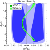
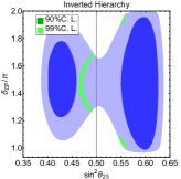
Figure 1: Regions of three-neutrino oscillation paramaters allowed at 90% and 99% of C. L. in the unconstrained global fit deSalas:2017kay (dark and light blue, respectively) and within the BMV scenario (dark and light green respectively). The left and right panels correspond to normal and inverted mass ordering, respectively.

In contrast with the general three-neutrino oscillation picture, we find that, taking into account the most recent global fit of neutrino oscillation paramaters deSalas:2017kay , the inverted mass ordering is only allowed at the 99% of C. L., an enhanced rejection than in the general unconstrained scenario. This is partly due to the fact that the preferred values of $\theta_{23}$ in the BMV case lie closer to maximality than in the general three-neutrino oscillation picture.

On the other hand, the strongly preferred normal ordering case has two solutions, one in each octant of $\theta_{23}$. Of these, one notices that there is only a small region in the higher octant, close to a CP-conserving value of the phase, $\delta_{CP}=\pi$. Although disfavored, this region is still allowed at 90% of C. L., as seen by the dark green region. In contrast, the preferred solution lies in the left octant, close to maximal CP violation. By comparing the dark green and dark blue regions one sees how the global analysis of the oscillation parameters within this model leads to an improved determination of $\theta_{23}$ and $\delta_{CP}$ when compared with the generic three-neutrino oscillation scenario. We now turn to the prospects of testing this model at future experimental setups.

3 Numerical analysis and new experiments

In order to determine the sensitivity of each experiment through numerical simulation, we use the GLoBES software as described in Huber:2004ka ; Huber:2007ji . Unless told otherwise, the true values of the oscillation parameters are assumed to be the best fit values obtained in deSalas:2017kay , see table 1. In accordance to recent global fit results, normal ordering has been assumed fixed throughout the simulation.

Parameters	deSalas:2017kay
$s^{2}_{12}$	$0.321^{+0.18}_{-0.16}$
$\theta_{12}(^{\circ})$	$34.5^{+1.1}_{-1.0}$
$s^{2}_{13}$	$0.0216^{+0.090}_{-0.075}$
$\theta_{13}(^{\circ})$	$8.44^{+0.18}_{-0.15}$
$\Delta m_{31}^{2}/10^{-3}({\rm eV}^{2})$	$2.55\pm 0.04$
$\Delta m_{21}^{2}/10^{-5}({\rm eV}^{2})$	$7.56\pm 0.19$
$s^{2}_{23}$	$0.43^{+0.20}_{-0.18}$
$\theta_{23}(^{\circ})$	$41.0\pm 1.1$
$\delta_{\rm CP}/\pi$	$1.40^{+0.31}_{-0.20}$

Table 1: General three-neutrino oscillation parameters taken from the most recent global fit deSalas:2017kay .

The sensitivity is calculated, at certain confidence levels, by using a Poissionian $\chi^{2}$ function Huber:2002mx ; Fogli:2002pt between the true dataset $x_{i}$ and the test dataset $y_{i}$,

$$\chi^{2}=\min\limits_{\{\xi_{a},\xi_{b}\}}\left[2\sum_{i=1}^{n}(y_{i}-x_{i}-x_{i}\ln\frac{y_{i}}{x_{i}})+\xi^{2}_{a}+\xi^{2}_{b}\right].$$ (6)

where $n$ is the total number of bins and $\xi_{a}$ and $\xi_{b}$ denote the pulls due to systematic errors. The test dataset is given by

$$y_{i}(\tilde{f},\xi_{a},\xi_{b})=N_{i}^{pre}(\tilde{f})\left[1+\pi^{a}\xi_{a}\right]+N_{i}^{b}(\tilde{f})\left[1+\pi^{b}\xi_{b}\right],$$ (7)

where $\tilde{f}$ is the set of oscillation parameters predicted by the model and $\pi^{a}$,$\pi^{b}$ are the systematic errors on signal and background respectively, assumed to be uncorrelated.

$N_{i}^{pre}$ and $N_{i}^{b}$ represent the number of predicted signal events and the background events in the $i$th energy bin, respectively. The true or observed data assumption from an experiment enter in Eq. 6 through

$$x_{i}(f)=N_{i}^{obs}(f)+N_{i}^{b}(f),$$ (8)

Now the total $\chi^{2}$ is calculated by combining various relevant channels,

$$\chi^{2}_{\rm total}=\underset{\nu_{\mu}\to\nu_{e}}{\chi^{2}}+\underset{\bar{\nu}_{\mu}\to\bar{\nu}_{e}}{\chi^{2}}+\underset{\nu_{\mu}\to\nu_{\mu}}{\chi^{2}}+\underset{\bar{\nu}_{\mu}\to\bar{\nu}_{\mu}}{\chi^{2}}\leavevmode\nobreak\ .$$ (9)

Finally this $\chi^{2}_{\rm total}$ is minimized over the free oscillation parameters ($\theta_{23},\theta_{13},\theta_{12}$, and $\delta_{CP}$) predicted by the model to get $\Delta\chi^{2}_{min}$. In order to map out the expectations for the octant and/or CP preference we assume only the four “well-measured” oscillation parameters (upper rows in Table 1) plus the indication in favor of normal mass ordering. Indeed, as seen above, the inverted mass ordering is only allowed at the 99% of C. L. In the next section we consider the case of a fit-independent global approach. We focus on two forthcoming experiments: the DUNE Acciarri:2015uup and T2HK experiments Abe:2015zbg , basing ourselves on their CDR report as briefly described below.

DUNE: The proposed DUNE experiment has a baseline of 1300 km and the far detector (FD) is placed at an on-axis location. In our simulation, a 40 kt liquid argon FD with 3.5 yrs. of $\nu$ run and 3.5 yrs. of $\bar{\nu}$ run was considered. The $\nu_{\mu}$ beam is generated by a 80 GeV proton beam delivered at 1.07 MW with a POT (protons on target) of $1.47\times 10^{21}$. The simulation for DUNE was done according to Acciarri:2015uup .

T2HK: The proposed T2HK experiment has a baseline of 295 km and the detector is placed at the same off-axis (0.8 degrees) location as in T2K. The idea is to upgrade the T2K experiment, with a much larger detector (560 kton fiducial mass) located in Kamioka, so that much larger statistics is ensured. We assume an integrated beam with power 7.5 MW $\times 10^{7}$ sec. which corresponds to $1.53\times 10^{22}$ POT. The ratio of the runtimes of $\nu$ and $\bar{\nu}$ mode was taken as $1:3$. The simulation for T2HK was performed according to Abe:2015zbg .

4 DUNE and T2HK sensitivities

As seen in deSalas:2017kay , the atmospheric angle $\theta_{23}$ and the CP phase $\delta_{CP}$ are the two most uncertain of the fundamental oscillation parameters. This is in agreement with other recent global fits of neutrino oscillations Forero:2014bxa ; Esteban:2016qun ; Capozzi:2017ipn . Theoretical scenarios, such as the BMV model, imply correlations between them. Thus, we now answer the very general and interesting questions: To what extent model correlations, such as the one predicted by the BMV model, can be tested by experimental data? Can one exhibit the rejection power of future experiments independently of any arbitrarily given choice for the parameters $\theta_{23}$ and $\delta_{CP}$ eventually chosen by nature?

Performing this exercise enables us to establish robust quantitative criteria capable of probing the model of interest, independently of any given input from neutrino oscillation fits. Fig. 2 answers the questions above, giving quantitative model-testing criteria valid irrespective of any assumed global neutrino oscillation fits.

Our simulation procedure has been set up as follows. In order to calculate the oscillation parameters predicted by the model and then fit them to the true data set, we have marginalized over the model parameters within their allowed range, for each true data set. Finally, we calculate the minimum $\Delta\chi^{2}$ at various confidence levels, as shown by the different colour combinations in Fig. 2. The cyan, blue, green, and orange bands correspond to the 1$\sigma$, 2$\sigma$, 3$\sigma$, and 4$\sigma$ confidence level of compatibility, at 1 degree of freedom, that is, $\Delta\chi^{2}$ = 1, 4, 9, and 16 respectively. The left panel gives the result for DUNE, while the right panel corresponds to T2HK. From this global-fit-independent sensitivity plot, one sees that DUNE can exclude, at $4\sigma$ statistical significance, the regions corresponding to $\sin^{2}\theta_{23}\gtrsim 0.59$ and $\sin^{2}\theta_{23}\lesssim 0.44$ without significant dependence on the value of $\delta_{CP}$ (TRUE). On the other hand, thanks to its higher statistics, T2HK has better sensitivity than DUNE and consequently can exclude even larger regions of parameter space. Notice that, as indicated in both panels, the best fit point obtained in deSalas:2017kay lies outside the corresponding 4$\sigma$ sensitivity regions at DUNE and T2HK, indicating how severely such parameter choice would be rejected by these experiments. We stress that these are robust model-testing criteria valid for any assumed global choice of neutrino oscillation parameters.

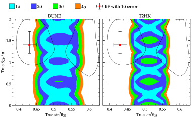
Figure 2: Expected sensitivity regions at various confidence levels at which DUNE (left) or T2HK (right) would test the revamped BMV model. The regions within the black bordered contours correspond to 90% C.L. and the red square is the current best fit value deSalas:2017kay . The full parameter scan of true values of $\sin^{2}\theta_{23}$ and $\delta_{CP}$ assumes normal neutrino mass ordering.

5 Summary and conclusion

Taking advantage of the latest global determination of neutrino oscillation parameters given in deSalas:2017kay we have investigated the status of the simplest revamped version of the BMV model for neutrino oscillation, proposed in Morisi:2013qna , as well as the chances of testing it further at future long-baseline neutrino experiments. To perform this task we have focussed on the sharp correlation between the “poorly determined” oscillation parameters $\theta_{23}$ and the phase $\delta_{CP}$ predicted in the model. We have determined the region of these oscillation parameters allowed within the BMV model, and compared it with what holds in the general three-neutrino oscillation scenario. We have found for this case a higher degree of rejection against the higher octant of $\theta_{23}$ than in the general unconstrained case. Through quantitative simulations of forthcoming experiments DUNE and T2HK, according to their technical proposals, we have also determined their potential for testing the BMV model. We have mapped out their sensitivity regions using only the values of the “well-measured” solar and atmospheric neutrino squared mass splittings, as well as the solar and reactor angle, plus the relatively strong preference for normal mass ordering that holds in the BMV scenario. We have also presented these results within a robust global approach valid for whatever the choice of $\theta_{23}$ and $\delta_{CP}$ is finally chosen by nature.

References

- (1) P. F. de Salas, D. V. Forero, C. A. Ternes, M. Tortola, and J. W. F. Valle, (2017), 1708.01186.
- (2) S. Morisi, D. Forero, J. C. Romao, and J. W. F. Valle, Phys.Rev. D88, 016003 (2013), 1305.6774.
- (3) C. Patrignani and P. D. Group, Chinese Physics C 40, 100001 (2016).
- (4) S. Boucenna, S. Morisi, M. Tortola, and J. W. F. Valle, Phys.Rev. D86, 051301 (2012), 1206.2555.
- (5) S. Roy, S. Morisi, N. N. Singh, and J. W. F. Valle, Phys. Lett. B748, 1 (2015), 1410.3658.
- (6) M. Hirsch et al., (2012), 1201.5525.
- (7) S. Morisi and J. W. F. Valle, Fortsch.Phys. 61, 466 (2013), 1206.6678.
- (8) H. Ishimori et al., An Introduction to Non-Abelian Discrete Symmetries for Particle PhysicistsLecture Notes in Physics (Springer, 2012).
- (9) S. F. King, A. Merle, S. Morisi, Y. Shimizu, and M. Tanimoto, New J.Phys. 16, 045018 (2014), 1402.4271.
- (10) P. Chen et al., JHEP 01, 007 (2016), 1509.06683.
- (11) P. Pasquini, S. C. Chuliá, and J. W. F. Valle, Phys. Rev. D95, 095030 (2017), 1610.05962.
- (12) S. Centelles Chuliá, R. Srivastava, and J. W. F. Valle, (2017), 1706.00210.
- (13) A. E. Cárcamo Hernández, S. Kovalenko, J. W. F. Valle, and C. A. Vaquera-Araujo, JHEP 07, 118 (2017), 1705.06320.
- (14) K. S. Babu, E. Ma, and J. W. F. Valle, Phys. Lett. B552, 207 (2003), hep-ph/0206292.
- (15) DUNE collaboration, R. Acciarri et al., (2015), 1512.06148.
- (16) Hyper-Kamiokande Proto-Collaboration, K. Abe et al., PTEP 2015, 053C02 (2015), 1502.05199.
- (17) P. Huber, M. Lindner, and W. Winter, Comput. Phys. Commun. 167, 195 (2005), hep-ph/0407333.
- (18) P. Huber, J. Kopp, M. Lindner, M. Rolinec, and W. Winter, Comput.Phys.Commun. 177, 432 (2007), hep-ph/0701187.
- (19) P. Huber, M. Lindner, and W. Winter, Nucl.Phys. B645, 3 (2002), hep-ph/0204352.
- (20) G. L. Fogli, E. Lisi, A. Marrone, D. Montanino, and A. Palazzo, Phys. Rev. D66, 053010 (2002), hep-ph/0206162.
- (21) D. Forero, M. Tortola, and J. W. F. Valle, Phys.Rev. D90, 093006 (2014), 1405.7540.
- (22) I. Esteban, M. C. Gonzalez-Garcia, M. Maltoni, I. Martinez-Soler, and T. Schwetz, JHEP 01, 087 (2017), 1611.01514.
- (23) F. Capozzi et al., Phys. Rev. D95, 096014 (2017), 1703.04471.