Limit cycles of discontinuous piecewise quadratic and cubic polynomial perturbations of a linear center

Abstract.

We apply the averaging theory of high order for computing the limit cycles of discontinuous piecewise quadratic and cubic polynomial perturbations of a linear center. These discontinuous piecewise differential systems are formed by two either quadratic, or cubic polynomial differential systems separated by a straight line.

We compute the maximum number of limit cycles of these discontinuous piecewise polynomial perturbations of the linear center, which can be obtained by using the averaging theory of order $n$ for $n=1,2,3,4,5$. Of course these limit cycles bifurcate from the periodic orbits of the linear center. As it was expected, using the averaging theory of the same order, the results show that the discontinuous quadratic and cubic polynomial perturbations of the linear center have more limit cycles than the ones found for continuous and discontinuous linear perturbations.

Moreover we provide sufficient and necessary conditions for the existence of a center or a focus at infinity if the discontinuous piecewise perturbations of the linear center are general quadratic polynomials or cubic quasi–homogenous polynomials.

1. Introduction and statement of the main Results

The interest on the dynamics of piecewise linear differential systems essentially started with the book of Andronov et al [1], whose Russian version appeared around the 1930’s. Due to the rich dynamics of the piecewise linear differential systems, and their applications in mechanics, electronics, economy, neuroscience, …, these systems have been studied by researchers from many different fields, see for instance the books of Bernardo et al [4] and of Simpson [26], the survey of Makarenkov and Lamb [23], and the references mentioned in all these works.

For the planar continuous piecewise linear differential systems with two zones separated by a straight line, Lum and Chua [21, 22] in 1991 conjectured that such differential systems have at most one limit cycle. In 1998 Freire, Ponce, Rodrigo and Torres [10] proved this conjecture.

While for the planar discontinuous piecewise linear differential systems with two zones separated by a straight line Han and Zhang [12] obtained differential systems having two limit cycles and conjectured that the maximum number of limit cycles of such class of differential systems is two. Huan and Yang [13] provided a numerical example of one of those differential system having three limit cycles. Inspired in this numerical example Llibre and Ponce [20] gave a proof of the existence of such three limit cycles in the class of these differential systems. Later on other authors also provide other discontinuous piecewise linear differential systems with two zones separated by a straight line also exhibiting three limit cycles, see [6, 7, 17]. More discussion about limit cycles of discontinuous piecewise differential systems can see references [28, 30].

Recently the averaging theory has been developed for studying the periodic solutions of the discontinuous piecewise differential systems. Thus Llibre, Mereu, Novaes and Teixeira [18, 19] extended the averaging theory up to order $1$ and $2$ for studying the periodic solutions of some discontinuous piecewise differential systems using techniques of regularization. Later on Itikawa, Llibre and Novaes [14] improved the averaging theory at any order for analyzing the periodic solutions of discontinuous piecewise differential systems.

We consider planar discontinuous piecewise differential systems having the line of discontinuity at $y=0$ of the form

(1) $$\begin{array}[]{l}\dot{x}=F^{\pm}(x,y,\varepsilon),\\ \dot{y}=G^{\pm}(x,y,\varepsilon),\end{array}$$

where

$$\begin{array}[]{lll}\dot{x}=F^{+}(x,y,\varepsilon)&=y+\displaystyle\sum_{j=1}^{n}~{}\varepsilon^{j}(a_{j0}+a_{j1}x+a_{j2}y+a_{j3}x^{2}+a_{j4}xy+a_{j5}y^{2}\\ &\qquad\qquad+a_{j6}x^{3}+a_{j7}x^{2}y+a_{j8}xy^{2}+a_{j9}y^{3}),\\ \dot{y}=G^{+}(x,y,\varepsilon)&=-x+\displaystyle\sum_{j=1}^{n}~{}\varepsilon^{j}(b_{j0}+b_{j1}x+b_{j2}y+b_{j3}x^{2}+b_{j4}xy+b_{j5}y^{2}\\ &\qquad\qquad+b_{j6}x^{3}+b_{j7}x^{2}y+b_{j8}xy^{2}+b_{j9}y^{3}),\end{array}$$

if $y\geq 0$, and

$$\begin{array}[]{lll}\dot{x}=F^{-}(x,y,\varepsilon)&=y+\displaystyle\sum_{j=1}^{n}~{}\varepsilon^{j}(A_{j0}+A_{j1}x+A_{j2}y+A_{j3}x^{2}+A_{j4}xy+A_{j5}y^{2}\\ &\qquad\qquad+A_{j6}x^{3}+A_{j7}x^{2}y+A_{j8}xy^{2}+A_{j9}y^{3}),\\ \dot{y}=G^{-}(x,y,\varepsilon)&=-x+\displaystyle\sum_{j=1}^{n}~{}\varepsilon^{j}(B_{j0}+B_{j1}x+B_{j2}y+B_{j3}x^{2}+B_{j4}xy+B_{j5}y^{2}\\ &\qquad\qquad+B_{j6}x^{3}+B_{j7}x^{2}y+B_{j8}xy^{2}+B_{j9}y^{3}),\end{array}$$

if $y\leq 0$, and where $n\in\mathbb{N}$, all parameters $a_{ji},b_{ji},A_{ji},B_{ji},\varepsilon\in\mathbb{R}$, and the perturbation parameter $|\varepsilon|$ is small enough. Here $\mathbb{N}$ is the set of positive integers and $\mathbb{R}$ is the set of real numbers. Notice that system (1) is a discontinuous piecewise differential system with the discontinuity straight line $y=0$. As usual the dot denotes derivative with respect to an independent real variable $t$.

In this paper we study the limit cycles of the discontinuous piecewise quadratic (i.e. when all the cubic monomials in (1) are zero) and cubic polynomial differential system (1), which bifurcate from the periodic orbits of the linear center $\dot{x}=y$, $\dot{y}=-x$. A classical problem for smooth differential systems is the weak 16th Hilbert problem, which essentially asks for the maximal number of limit cycles that bifurcate from the periodic orbits of a center when this is perturbed inside a class of polynomial differential systems with a fixed degree, see for more details [2, 3, 15, 27]. Here we are extending this problem to the non–smooth differential system (1).

We denote by $L_{2}(n)$ and $L_{3}(n)$ the maximum number of limit cycles of the discontinuous piecewise polynomial differential system (1) with degree $2$ and $3$ respectively which can be obtained using the averaging theory of order $n$ described in section 2. Then we have the following results.

Theorem 1.

For $n=1,2,3,4,5$ we have that $L_{2}(n)=2,3,5,6,8$, and $L_{3}(n)=3,5,8,11,13$, respectively.

Iliev in [16] studied the maximum number of limit cycles $L_{I}(n)$ coming from the perturbation of the linear center $\dot{x}=y,~{}\dot{y}=-x$ when this center is perturbed inside the class of all polynomial differential systems of degree $n$. Buzzi, Pessoa and Torregrosa in [7] found the maximum number of limit cycles $L_{1}(n)$, that bifurcate from the periodic orbits of the linear center $\dot{x}=y,~{}\dot{y}=-x$ when this center is perturbed inside the class of all discontinuous piecewise linear differential systems separated by a straight line. Their results for $n=1,2,3,4,5$ together with the results of Theorem 1 are given in Table 1.

Order $n$	$L_{1}(n)$	$L_{2}(n)$	$L_{3}(n)$	$L_{I}(n)$
1	1	2	3	0
2	1	3	5	1
3	2	5	8	1
4	3	6	11	2
5	3	8	13	2

Table 1. Maximum number of limit cycles bifurcating from the periodic orbits of the linear center using averaging theory of order $n$.

If there exists a neighborhood of the infinity in the Poincaré disc [9, Chapter 5] filled of periodic orbits, then we say that system (1) has a center at infinity. If there exists a neighborhood of the infinity in the Poincaré disc where all the orbits spiral going to or coming from the infinity, then we say that system (1) has a focus at infinity. We shall investigate the problem of the existence of a center or a focus at infinity under small perturbations, but before we need some definitions.

A planar polynomial differential system

(2) $$\dot{x}=P(x,y),\qquad\qquad\dot{y}=Q(x,y),$$

where $P(x,y)$ and $Q(x,y)$ are non–zero polynomials, is quasi–homogeneous if there exist $s_{1},s_{2},d\in\mathbb{N}$ such that for all positive number $\alpha$ they satisfy

$$P(\alpha^{s_{1}}x,\alpha^{s_{2}}y)=\alpha^{s_{1}+d-1}P(x,y),\ \ \ \ Q(\alpha^{s_{1}}x,\alpha^{s_{2}}y)=\alpha^{s_{2}+d-1}Q(x,y),$$

Then as usual $(s_{1},s_{2})$ are the weight exponents, $d$ is the weight degree with respect to the weight exponents, and $w=(s_{1},s_{2},d)$ is the weight vector of the quasi–homogeneous polynomial differential system (2).

By Proposition 19 of Giné, Grau and Llibre [11], an irreducible quasi-homogeneous but non-homogeneous cubic ordinary polynomial differential system can be written in one of the following forms:

$$(I) ~{}\dot{x}=y(a_{1}x+b_{1}y^{2}),~{}\dot{y}=c_{1}x+d_{1}y^{2},\mbox{\it with}~{}b_{1}c_{1}\neq 0.$$

$$(II) ~{}\dot{x}=a_{2}x^{2}+b_{2}y^{3},~{}\dot{y}=c_{2}xy,~{}\mbox{\it with}~{}a_{2}b_{2}c_{2}\neq 0.$$

$$(III) ~{}\dot{x}=a_{3}y^{3},~{}\dot{y}=b_{3}x^{2}~{}\mbox{\it with}~{}a_{3}b_{3}\neq 0.$$

$$(IV) ~{}\dot{x}=x(a_{4}x+b_{4}y^{2}),~{}\dot{y}=y(c_{4}x+d_{4}y^{2}),~{}\mbox{\it with}~{}a_{4}d_{4}\neq 0.$$

$$(V) ~{}\dot{x}=a_{5}xy^{2},~{}\dot{y}=b_{5}x^{2}+c_{5}y^{3},~{}\mbox{\it with}~{}a_{5}b_{5}c_{5}\neq 0.$$

$$(VI) ~{}\dot{x}=a_{6}xy^{2},~{}\dot{y}=b_{6}x+c_{6}y^{3},~{}\mbox{\it with }~{}a_{6}b_{6}c_{6}\neq 0.$$

$$(VII) ~{}\dot{x}=a_{7}x+b_{7}y^{3},~{}\dot{y}=c_{7}y,~{}\mbox{\it with}~{}a_{7}b_{7}c_{7}\neq 0.$$

Perturbing the linear center by discontinuous cubic quasi-homogenous but non-homogeneous polynomials, we obtain the following $7$ systems:

(3) $$\begin{array}[]{l}\dot{x}=y+~{}\varepsilon y(a_{1}x+b_{1}y^{2}),~{}~{}\dot{y}=-x+~{}\varepsilon(c_{1}x+d_{1}y^{2})~{}\mbox{\it if}~{}y\geq 0,\\ \dot{x}=y+~{}\varepsilon y(A_{1}x+B_{1}y^{2}),~{}~{}\dot{y}=-x+~{}\varepsilon(C_{1}x+D_{1}y^{2})~{}\mbox{\it if}~{}y\leq 0\end{array}$$

where $b_{1}c_{1}B_{1}C_{1}\neq 0$,

(4) $$\begin{array}[]{l}\dot{x}=y+~{}\varepsilon a_{2}x^{2}+b_{2}y^{3},~{}~{}\dot{y}=-x+~{}\varepsilon c_{2}xy~{}\mbox{\it if}~{}y\geq 0,\\ \dot{x}=y+~{}\varepsilon A_{2}x^{2}+B_{2}y^{3},~{}~{}\dot{y}=-x+~{}\varepsilon C_{2}xy~{}\mbox{\it if}~{}y\leq 0,\end{array}$$

where $a_{2}b_{2}c_{2}A_{2}B_{2}C_{2}\neq 0$,

(5) $$\begin{array}[]{l}\dot{x}=y+~{}\varepsilon a_{3}y^{3},~{}~{}\dot{y}=-x+~{}\varepsilon b_{3}x^{2}~{}\mbox{\it if}~{}y\geq 0,\\ \dot{x}=y+~{}\varepsilon A_{3}y^{3},~{}~{}\dot{y}=-x+~{}\varepsilon B_{3}x^{2}~{}\mbox{\it if}~{}y\leq 0,\end{array}$$

where $a_{3}b_{3}A_{3}B_{3}\neq 0$,

(6) $$\begin{array}[]{l}\dot{x}=y+~{}\varepsilon x(a_{4}x+b_{4}y^{2}),~{}~{}\dot{y}=-x+~{}\varepsilon y(c_{4}x+d_{4}y^{2})~{}\mbox{\it if}~{}y\geq 0,\\ \dot{x}=y+~{}\varepsilon x(A_{4}x+B_{4}y^{2}),~{}~{}\dot{y}=-x+~{}\varepsilon y(C_{4}x+D_{4}y^{2})~{}\mbox{\it if}~{}y\leq 0,\end{array}$$

where $a_{4}d_{4}A_{4}D_{4}\neq 0$,

(7) $$\begin{array}[]{l}\dot{x}=y+~{}\varepsilon a_{5}xy^{2},~{}~{}\dot{y}=-x+~{}\varepsilon b_{5}x^{2}+c_{5}y^{3}~{}\mbox{\it if}~{}y\geq 0,\\ \dot{x}=y+~{}\varepsilon A_{5}xy^{2},~{}~{}\dot{y}=-x+~{}\varepsilon B_{5}x^{2}+C_{5}y^{3}~{}\mbox{\it if}~{}y\leq 0,\end{array}$$

where $a_{5}b_{5}c_{5}A_{5}B_{5}C_{5}\neq 0$,

(8) $$\begin{array}[]{l}\dot{x}=y+~{}\varepsilon a_{6}xy^{2},~{}~{}\dot{y}=-x+~{}\varepsilon b_{6}x+c_{6}y^{3}~{}\mbox{\it if}~{}y\geq 0,\\ \dot{x}=y+~{}\varepsilon A_{6}xy^{2},~{}~{}\dot{y}=-x+~{}\varepsilon B_{6}x+C_{6}y^{3}~{}\mbox{\it if}~{}y\leq 0,\end{array}$$

and $a_{6}b_{6}c_{6}A_{6}B_{6}C_{6}\neq 0$, and

(9) $$\begin{array}[]{l}\dot{x}=y+~{}\varepsilon(a_{7}x+b_{7}y^{3}),~{}~{}\dot{y}=-x+~{}\varepsilon c_{7}y~{}\mbox{\it if}~{}y\geq 0,\\ \dot{x}=y+~{}\varepsilon(A_{7}x+B_{7}y^{3}),~{}~{}\dot{y}=-x+~{}\varepsilon C_{7},~{}\mbox{\it if}~{}y\leq 0,\end{array}$$

where $a_{7}b_{7}c_{7}A_{7}B_{7}C_{7}\neq 0$.

A center is called a global center when the periodic orbits surrounding the center filled the whole plain except the center itself.

Theorem 2.

Assume $n=1$ in system (1).

• System (1) has neither centers nor foci at infinity if the discontinuous polynomial perturbations are of degree $2$ (i.e. if $a_{ji}=b_{ji}=A_{ji}=B_{ji}=0$ for $i=6,...,9$).

• The unique systems from (3) to (9) which can have a center or a focus at infinity are the systems (3) or (9).

• The infinity of system (9) is a focus. System (3) has a focus or a center at infinity if $-b_{1}\varepsilon<0$ and $-B_{1}\varepsilon<0$, and it has a center at infinity if $-b_{1}\varepsilon<0$, $-B_{1}\varepsilon<0$, $a_{1}=-2d_{1}$ and $A_{1}=0=D_{1}$, which is a global center.

2. Averaging theory and the Descartes Theorem

Using the polar coordinates $(r,\theta)$ such that $x=r\cos\theta$ and $y=r\sin\theta$, the differential system (1) in these coordinates becomes

(10) $$\dfrac{dr}{d\theta}=\left\{\begin{array}[]{l}P^{+}(\theta,r,\varepsilon)\quad\textrm{if}\quad 0\leq\theta\leq\pi,\vspace{0.2cm}\\ P^{-}(\theta,r,\varepsilon)\quad\textrm{if}\quad-\pi\leq\theta\leq 0,\end{array}\right.$$

where $P^{\pm}(\theta,r,\varepsilon)=\sum_{j=1}^{k}\varepsilon^{j}P_{j}^{\pm}(\theta,r)+\varepsilon^{k+1}Q^{\pm}(\theta,r,\varepsilon)$ with $k\in\mathbb{N}$, $\theta\in\mathbb{S}^{1}$ and $r\in\mathbb{R}_{+}$, the functions $P_{j}^{\pm}:\mathbb{S}^{1}\times\mathbb{R}_{+}\rightarrow\mathbb{R}$ for $j=1,2,\ldots,k,$ and $Q^{\pm}:\mathbb{S}^{1}\times\mathbb{R}_{+}\times(-\varepsilon_{0},\varepsilon_{0})\rightarrow\mathbb{R}$ are analytic. Here $\varepsilon_{0}>0$ and $\mathbb{R}_{+}=[0,\infty)$.

The averaged function $f_{j}:\mathbb{R}_{+}\rightarrow\mathbb{R}$ of order $j$ for the differential equation (10) is defined as

(11) $$f_{j}(r)=\dfrac{y^{+}_{j}(\pi,r)-y^{-}_{j}(-\pi,r)}{j!},\quad j=1,2,\ldots,k,$$

where $y_{j}^{\pm}$ for $j=1,2,3,4,5$ are

$$y^{\pm}_{1}(\theta,r)= \displaystyle\int_{0}^{\theta}P^{\pm}_{1}(\phi,r)d\phi,\vspace{0.1cm}$$

$$y^{\pm}_{2}(\theta,r)= \displaystyle\int_{0}^{\theta}\Big{(}2P^{\pm}_{2}(\phi,r)+2\partial P^{\pm}_{1}(\phi,r)y^{\pm}_{1}(\phi,r)\Big{)}d\phi,\vspace{0.1cm}$$

$$y^{\pm}_{3}(\theta,r)= \displaystyle\int_{0}^{\theta}\Big{(}6P^{\pm}_{3}(\phi,r)+6\partial P^{\pm}_{2}(\phi,r)y^{\pm}_{1}(\phi,r)$$

$$+3\partial^{2}P^{\pm}_{1}(\phi,r)y^{\pm}_{1}(\phi,r)^{2}+3\partial P^{\pm}_{1}(\phi,r)\,y^{\pm}_{2}(\phi,r)\Big{)}d\phi,\vspace{0.1cm}$$

(12) $$y^{\pm}_{4}(\theta,r)= \displaystyle\int_{0}^{\theta}\Big{(}24P^{\pm}_{4}(\phi,r)+24\partial P^{\pm}_{3}(\phi,r)y^{\pm}_{1}(\phi,r)$$

$$+12\partial^{2}P^{\pm}_{2}(\phi,r)y^{\pm}_{1}(\phi,r)^{2}+12\partial P^{\pm}_{2}(\phi,r)y^{\pm}_{2}(\phi,r)$$

$$+12\partial^{2}P^{\pm}_{1}(\phi,r)y^{\pm}_{1}(\phi,r)y^{\pm}_{2}(\phi,r)$$

$$+4\partial^{3}P^{\pm}_{1}(\phi,r)y^{\pm}_{1}(\phi,r)^{3}+4\partial P^{\pm}_{1}(\phi,r)y^{\pm}_{3}(\phi,r)\Big{)}d\phi,\vspace{0.1cm}$$

$$y^{\pm}_{5}(\theta,r)= \displaystyle\int_{0}^{\theta}\Big{(}120P^{\pm}_{5}(\phi,r)+120\partial P^{\pm}_{4}(\phi,r)y^{\pm}_{1}(\phi,r)$$

$$+60\partial^{2}P^{\pm}_{3}(\phi,r)y^{\pm}_{1}(\phi,r)^{2}+60\partial P^{\pm}_{3}(\phi,r)y^{\pm}_{2}(\phi,r)$$

$$+60\partial^{2}P^{\pm}_{2}(\phi,r)y^{\pm}_{1}(\phi,r)y^{\pm}_{2}(\phi,r)+20\partial^{3}P^{\pm}_{2}(\phi,r)y^{\pm}_{1}(\phi,r)^{3}$$

$$+20\partial P^{\pm}_{2}(\phi,r)y^{\pm}_{3}(\phi,r)+20\partial^{2}P^{\pm}_{1}(\phi,r)y^{\pm}_{1}(\phi,r)y^{\pm}_{3}(\phi,r)$$

$$+15\partial^{2}P^{\pm}_{1}(\phi,r)y^{\pm}_{2}(\phi,r)^{2}+30\partial^{3}P^{\pm}_{1}(\phi,r)y^{\pm}_{1}(\phi,r)^{2}y^{\pm}_{2}(\phi,r)$$

$$+5\partial^{4}P^{\pm}_{1}(\phi,r)y^{\pm}_{1}(\phi,r)^{4}+5\partial P^{\pm}_{1}(\phi,r)y^{\pm}_{4}(\phi,r)\Big{)}d\phi.$$

From [14] we have the following result.

Theorem 3.

Suppose that $j$ is the first integer such that the averaged function $f_{i}=0$ for $i=1,2,\ldots,j-1$ and $f_{j}\neq 0$. If there is $r^{*}\in\mathbb{R}_{+}$ such that $f_{j}(r^{*})=0$ and $f^{\prime}_{j}(r^{*})\neq 0,$ then for $|\varepsilon|\neq 0$ small enough there is a $2\pi$–periodic solution $r(\theta,\varepsilon)$ of (10) such that $r(0,\varepsilon)\to r^{*}$ when $\varepsilon\to 0$.

Note that the simple positive zeros of the averaged function $f_{j}$ provides limit cycles of the differential equation (10).

We shall use the following version of the Descartes Theorem as it is proved in [5].

Theorem 4 (Descartes theorem).

Consider the real polynomial $p(x)=a_{i_{1}}x^{i_{1}}+a_{i_{2}}x^{i_{2}}+\ldots+a_{i_{r}}x^{i_{r}}$ with $0=i_{1}<i_{2}<\ldots<i_{r}$. If $a_{i_{j}}a_{i_{j+1}}<0,$ we say that we have a variation of sign. If the number of variations of signs is $m,$ then the polynomial $p(x)$ has at most $m$ positive real roots. Furthermore, always we can choose the coefficients of the polynomial $p(x)$ in such a way that $p(x)$ has exactly $r-1$ positive real roots.

3. Proof of Theorem 1

We write the discontinuous piecewise cubic polynomial differential system (1) in polar coordinates, obtaining a differential system $(\dot{r},\dot{\theta})$. After taking $\theta$ as the new independent variable we get a differential equation $dr/d\theta$, and doing Taylor series expansion of $dr/d\theta$ with respect to the variable $\varepsilon$ at $\varepsilon=0$ we obtain the differential equation (10) associated to system (1).

Since system (1) is a polynomial differential system, the functions $P_{j}^{\pm}(\theta,r)$ and $Q_{j}^{\pm}(\theta,r,\varepsilon)$ are analytic. Moreover the differential equation $dr/d\theta$ in the form (10) is $2\pi-$periodic because the variable $\theta$ appears through the sinus and cosinus functions. In order to apply Theorem 3 to our differential equation $dr/d\theta$ it suffices to take an open interval $\mathcal{D}=\{r:0<r<r_{0}\}\subset\mathbb{R}_{+}$, where the unperturbed system can have periodic orbits $r(\theta)$ such that $r(0)=r$ with $0<r<r_{0}.$ Here we only give the explicit expressions of

$$P_{1}^{+}(a_{ij},b_{ij},\theta,r)= \frac{1}{8}\bigg{(}r^{3}\Big{(}4b_{19}\cos(2\theta)-2b_{18}\sin(2\theta)+a_{19}\sin(4\theta)-a_{17}\sin(4\theta)$$

$$~{}-4a_{16}\cos(2\theta)-2a_{17}\sin(2\theta)+b_{18}\sin(4\theta)+a_{18}\cos(4\theta)$$

$$~{}-2a_{19}\sin(2\theta)+b_{17}\cos(4\theta)-a_{16}\cos(4\theta)-2b_{16}\sin(2\theta)$$

$$~{}-b_{16}\sin(4\theta)-b_{19}\cos(4\theta)-a_{18}-3a_{16}-3b_{19}-b_{17}\Big{)}$$

$$~{}+r^{2}\Big{(}2b_{15}\sin(3\theta)-2a_{14}\sin(3\theta)-2b_{14}\cos\theta-2a_{14}\sin\theta$$

$$~{}-2b_{13}\sin(3\theta)-6a_{13}\cos\theta+2b_{14}\cos(3\theta)-2a_{13}\cos(3\theta)$$

$$~{}+2a_{15}\cos(3\theta)-2b_{13}\sin\theta-2a_{15}\cos\theta-6b_{15}\sin\theta\Big{)}$$

$$~{}+r\Big{(}-4a_{12}\sin(2\theta)-4a_{11}\cos(2\theta)-4a_{11}+4b_{12}\cos(2\theta)$$

$$~{}-4b_{11}\sin(2\theta)-4b_{12}\Big{)}-b_{10}\sin\theta-a_{10}\cos\theta\bigg{)},$$

$$P_{2}^{+}(a_{ij},b_{ij},\theta,r)= -a_{20}\cos\theta-b_{20}\sin\theta-\Big{(}b_{22}-(b_{22}-a_{21})\cos^{2}\theta+(a_{22}+b_{21})\sin\theta\cos\theta\Big{)}r$$

$$~{}+\Big{(}-b_{25}\sin\theta-(b_{24}+a_{25})\cos\theta-(a_{24}+b_{23}-b_{25})\sin\theta\cos^{2}\theta$$

$$~{}+(a_{25}-a_{23}+b_{24})\cos^{3}\theta\Big{)}r^{2}+\Big{(}-b_{29}-(a_{29}+b_{28})\sin\theta\cos\theta$$

$$~{}+(2b_{29}-a_{28}-b_{27})\cos^{2}\theta+(b_{28}+a_{29}-a_{27}-b_{26})\sin\theta\cos^{3}\theta$$

$$~{}+(b_{27}-b_{29}-a_{26}+a_{28})\cos^{4}\theta\Big{)}r^{3}~{}-\Big{(}b_{10}\sin\theta+a_{10}\cos\theta$$

$$~{}+(b_{12}+(b_{11}+a_{12})\sin\theta\cos\theta+(a_{11}-b_{12})\cos^{2}\theta)r+((a_{15}+b_{14})\cos\theta$$

$$~{}+b_{15}\sin\theta+(b_{13}+a_{14}-b_{15})\sin\theta\cos^{2}\theta+(a_{13}-b_{14}-a_{15})\cos^{3}\theta)r^{2}$$

$$~{}+(b_{19}+(b_{18}+a_{19})\sin\theta\cos\theta+(a_{18}-2b_{19}+b_{17})\cos^{2}\theta$$

$$~{}+(b_{19}-a_{18}-b_{17}+a_{16})\cos^{4}\theta+(a_{17}+b_{16}-a_{19}-b_{18})\sin\theta\cos^{3}\theta)r^{3}\Big{)}$$

$$~{}\Big{(}b_{10}\cos\theta-a_{10}\sin\theta+(-a_{12}+(b_{12}-a_{11})\sin\theta\cos\theta+(a_{12}+b_{11})\cos^{2}\theta)r$$

$$~{}+(-a_{15}\sin\theta+(b_{15}-a_{14})\cos\theta+(a_{15}+b_{14}-a_{13})\sin\theta\cos^{2}\theta$$

$$~{}+(b_{13}-b_{15}+a_{14})\cos^{3}\theta)r^{2}~{}+(-a_{19}+(b_{18}+2a_{19}-a_{17})\cos^{2}\theta$$

$$~{}+(b_{19}-a_{18})\sin\theta\cos\theta+(b_{17}-a_{16}-b_{19}+a_{18})\sin\theta\cos^{3}\theta$$

$$~{}+(b_{16}-b_{18}+a_{17}-a_{19})\cos^{4}\theta)r^{3}\Big{)}/r.$$

We omit the explicit expressions of $P_{k}^{+}(a_{ij},b_{ij},\theta,r)$ for $k=3,4,5$ because they are quite large. Moreover, we have

$$P_{k}^{-}(A_{ij},B_{ij},\theta,r)= P_{k}^{+}(a_{ij},b_{ij},\theta,r),$$

for $k=1,2,3,4,5$.

From (12) we compute the functions $y_{j}^{+}(\theta,r)$ and $y_{j}^{-}(\theta,r)$ for $j=1,\dots,5$. After we compute the averaged functions $f_{j}(r)$ for $j=1,\dots,5$ by using formulas (11). Thus the averaged function of first order is

$$f_{1}(r)=\eta_{13}r^{3}+\eta_{12}r^{2}+\eta_{11}r+\eta_{10},$$

where

$$\eta_{13}= \frac{\pi}{8}\big{(}-A_{18}-B_{17}-3A_{16}-3B_{19}-b_{17}-a_{18}-3b_{19}-3a_{16}\big{)},$$

$$\eta_{12}= \frac{2}{3}\big{(}-b_{13}+A_{14}+2B_{15}-2b_{15}-a_{14}+B_{13}\big{)},$$

$$\eta_{11}= \frac{\pi}{2}\big{(}-B_{12}-a_{11}-b_{12}-A_{11}\big{)},$$

$$\eta_{10}= -2b_{10}+2B_{10}.$$

The rank of the Jacobian matrix of the function $M_{1}=(\eta_{13},\eta_{12},\eta_{11},\eta_{10})$ with respect to the parameters $a_{1i},b_{1i},A_{1i},B_{1i}$, $i=0,1,..,9$ is maximal, i.e. it is $4$. Then the coefficients $\eta_{13},\eta_{12}$, $\eta_{11}$ and $\eta_{10}$ are linearly independent in their variables. Clearly $f_{1}(r)=0$ has at most three solutions in $\mathcal{D}$. Thus, by Theorems 3 and 4 it follows that at most $3$ limit cycles can bifurcate from the periodic orbits of the linear system using the averaging theory of first order, and from the last part of Theorem 4 there are systems (1) with three limit cycles.

Solving $\eta_{13}$ for $A_{16}$, $\eta_{12}$ for $B_{15}$, $\eta_{11}$ for $B_{12}$ and $\eta_{10}$ for $B_{10}$, we obtain that $f_{1}(r)\equiv 0$. Applying the averaging theory of order two, we get the second averaged function

$$f_{2}(r)=\eta_{25}r^{5}+\eta_{24}r^{4}+\eta_{23}r^{3}+\eta_{22}r^{2}+\eta_{21}r+\eta_{20},$$

where

$$\eta_{25}= \frac{\pi}{128}\big{(}18\pi a_{16}a_{18}-2A_{16}B_{18}-30A_{16}B_{16}-6B_{17}B_{18}-10B_{17}B_{16}-3A_{18}^{2}\pi$$

$$~{}-18B_{17}B_{19}\pi-18A_{16}A_{18}\pi-54A_{16}B_{19}\pi-6A_{18}B_{17}\pi-18A_{18}B_{19}\pi$$

$$~{}+18\pi a_{18}b_{19}+6\pi a_{18}b_{17}-3B_{17}^{2}\pi-27B_{19}^{2}\pi-27A_{16}^{2}\pi+3\pi a_{18}^{2}+27\pi a_{16}^{2}$$

$$~{}-6b_{19}b_{16}+27\pi b_{19}^{2}+3\pi b_{17}^{2}-2B_{17}A_{17}+2B_{17}A_{19}+6a_{18}a_{17}-2a_{18}b_{16}$$

$$~{}+6a_{16}a_{19}+2b_{17}a_{19}-2b_{17}a_{17}-10b_{17}b_{16}-6b_{17}b_{18}+2b_{19}a_{17}+2a_{18}b_{18}$$

$$~{}+54\pi a_{16}b_{19}+18\pi a_{16}b_{17}-10b_{19}b_{18}+10a_{18}a_{19}+30b_{19}a_{19}-30a_{16}b_{16}$$

$$~{}-2a_{16}b_{18}+10a_{16}a_{17}+18\pi b_{17}b_{19}-18A_{16}B_{17}\pi-2A_{18}B_{16}+6A_{18}A_{17}$$

$$~{}+10A_{18}A_{19}-6B_{19}B_{16}+2B_{19}A_{17}+2A_{18}B_{18}+10A_{16}A_{17}+6A_{16}A_{19}$$

$$~{}+30B_{19}A_{19}-10B_{19}B_{18}\big{)},$$

$$\eta_{24}= \frac{1}{2}\big{(}16B_{14}B_{17}/45-8a_{17}b_{15}/15+8a_{18}b_{14}/45+16a_{19}b_{15}/15-4b_{13}b_{16}/3$$

$$~{}-8A_{15}A_{16}/15+8B_{13}B_{18}/15-16b_{15}b_{16}/15-16b_{14}b_{17}/45-8b_{13}b_{18}/15$$

$$~{}+4B_{13}B_{16}/3-8A_{15}B_{17}/45+8A_{17}B_{15}/15+8A_{17}B_{13}/15+8a_{14}a_{19}/15$$

$$~{}-4A_{13}B_{17}/45-28A_{13}A_{16}/15-8A_{13}A_{18}/9-8a_{14}b_{16}/15+4a_{13}b_{17}/45$$

$$~{}+4A_{16}B_{14}/15-32A_{15}B_{19}/15-16A_{19}B_{15}/15+16B_{15}B_{16}/15$$

$$~{}+8a_{15}a_{16}/15+8a_{13}b_{19}/5+4a_{14}a_{17}/15-8A_{13}B_{19}/5+8A_{14}B_{16}/15$$

$$~{}-8A_{18}B_{14}/45-8A_{14}A_{19}/15+16B_{15}B_{18}/15-32A_{15}A_{18}/45$$

$$~{}+32a_{15}a_{18}/45+28a_{13}a_{16}/15+8a_{13}a_{18}/9+8a_{15}b_{17}/45+32a_{15}b_{19}/15$$

$$~{}-4a_{16}b_{14}/15-16b_{15}b_{18}/15-8a_{17}b_{13}/15+5\pi a_{18}b_{13}/12-4A_{14}A_{17}/15$$

$$~{}+5\pi b_{15}b_{19}/2+5\pi b_{13}b_{17}/12+5\pi a_{14}a_{16}/4+5\pi a_{18}b_{15}/6$$

$$~{}+5\pi b_{13}b_{19}/4+5\pi b_{15}b_{17}/6+5\pi a_{14}a_{18}/12+5A_{16}B_{13}\pi/4$$

$$~{}+5A_{18}B_{15}\pi/6+5A_{14}B_{17}\pi/12+5A_{14}A_{18}\pi/12+5A_{16}B_{15}\pi/2$$

$$~{}+5A_{14}B_{19}\pi/4+5A_{14}A_{16}\pi/4+5B_{15}B_{19}\pi/2+5A_{18}B_{13}\pi/12$$

$$~{}+5B_{15}B_{17}\pi/6+5B_{13}B_{19}\pi/4+5B_{13}B_{17}\pi/12+5\pi a_{14}b_{17}/12$$

$$~{}+5\pi a_{14}b_{19}/4+5\pi a_{16}b_{13}/4+5\pi a_{16}b_{15}/2\big{)},$$

$$\eta_{23}= \frac{1}{2}\big{(}32a_{14}b_{15}/9-32B_{15}^{2}/9-8A_{14}^{2}/9-8B_{13}^{2}/9+16a_{14}b_{13}/9-B_{27}\pi/4$$

$$~{}-32B_{13}B_{15}/9+32b_{13}b_{15}/9-16A_{14}B_{13}/9-32A_{14}B_{15}/9-A_{28}\pi/4$$

$$~{}-3B_{29}\pi/4-3A_{26}\pi/4-b_{27}\pi/4-a_{28}\pi/4-3a_{26}\pi/4+3\pi^{2}a_{16}b_{12}/4$$

$$~{}-3b_{29}\pi/4+32b_{15}^{2}/9-\pi a_{11}b_{18}/16+3\pi^{2}a_{11}b_{19}/4-11A_{11}B_{16}\pi/16$$

$$~{}+\pi^{2}a_{18}b_{12}/4-A_{11}B_{17}\pi^{2}/4-3A_{11}B_{19}\pi^{2}/4-3A_{16}B_{12}\pi^{2}/4$$

$$~{}-3A_{11}A_{16}\pi^{2}/4-3B_{12}B_{19}\pi^{2}/4-B_{12}B_{17}\pi^{2}/4-A_{18}B_{12}\pi^{2}/4$$

$$~{}-A_{11}A_{18}\pi^{2}/4+A_{12}B_{17}\pi/8+A_{18}B_{11}\pi/8-B_{14}B_{13}\pi/4+8a_{14}^{2}/9$$

$$~{}-A_{11}B_{18}\pi/16-7A_{17}B_{12}\pi/16+3A_{18}A_{12}\pi/8+3A_{11}A_{19}\pi/16$$

$$~{}+\pi^{2}a_{11}a_{18}/4+\pi^{2}a_{11}b_{17}/4+3a_{16}a_{12}\pi/8-b_{17}b_{11}\pi/8+8b_{13}^{2}/9$$

$$~{}+\pi^{2}b_{12}b_{17}/4+3\pi^{2}b_{12}b_{19}/4+\pi a_{12}b_{17}/8+\pi a_{18}b_{11}/8+A_{14}A_{13}\pi/4$$

$$~{}-7\pi a_{17}b_{12}/16-11b_{12}b_{16}\pi/16+3A_{16}A_{12}\pi/8+A_{11}A_{17}\pi/16$$

$$~{}+A_{14}A_{15}\pi/4-A_{13}B_{13}\pi/2+9b_{19}a_{12}\pi/8-b_{14}b_{15}\pi/4+3b_{12}a_{19}\pi/16$$

$$~{}-11B_{12}B_{16}\pi/16+3B_{12}A_{19}\pi/16-B_{17}B_{11}\pi/8+3B_{19}B_{11}\pi/8$$

$$~{}-9B_{12}B_{18}\pi/16+9B_{19}A_{12}\pi/8+3a_{18}a_{12}\pi/8-11a_{11}b_{16}\pi/16$$

$$~{}+a_{11}a_{17}\pi/16-3a_{16}b_{11}\pi/8+3b_{19}b_{11}\pi/8+a_{15}a_{14}\pi/4-B_{14}B_{15}\pi/4$$

$$~{}+a_{15}b_{15}\pi/2-b_{14}b_{13}\pi/4-b_{13}a_{13}\pi/2+a_{14}a_{13}\pi/4-9b_{12}b_{18}\pi/16$$

$$~{}-3A_{16}B_{11}\pi/8+B_{15}A_{15}\pi/2+3\pi^{2}a_{11}a_{16}/4+3a_{11}a_{19}\pi/16\big{)},$$

$$\eta_{22}= \frac{1}{2}\big{(}4B_{23}/3-4a_{24}/3-4b_{23}/3-8b_{25}/3+4A_{24}/3+8B_{25}/3-4b_{11}b_{13}/3$$

$$~{}-4A_{12}A_{14}/3-16b_{12}b_{14}/9+8a_{12}b_{15}/3-20a_{13}b_{12}/9-8A_{12}B_{15}/3$$

$$~{}+8a_{11}a_{15}/9-4a_{11}b_{14}/9-8A_{15}B_{12}/9-8a_{17}b_{10}/3+4a_{11}a_{13}/9$$

$$~{}-8b_{10}b_{18}/3-4b_{10}b_{16}+8a_{10}b_{19}+4a_{12}a_{14}/3+8a_{10}a_{18}/3+4a_{10}b_{17}/3$$

$$~{}+8A_{17}B_{10}/3+16B_{12}B_{14}/9-4A_{10}B_{17}/3-8A_{10}B_{19}+4B_{11}B_{13}/3$$

$$~{}-8A_{10}A_{18}/3+8B_{10}B_{18}/3+4B_{10}B_{16}+4A_{11}B_{14}/9+20A_{13}B_{12}/9$$

$$~{}-8A_{11}A_{15}/9-4A_{11}A_{13}/9-4A_{10}A_{16}+8a_{15}b_{12}/9+4a_{10}a_{16}+\pi a_{11}a_{14}$$

$$~{}+\pi a_{11}b_{13}+\pi a_{14}b_{12}+\pi b_{12}b_{13}+3a_{18}b_{10}\pi/4+9a_{16}b_{10}\pi/4+3b_{10}b_{17}\pi/4$$

$$~{}+2\pi b_{12}b_{15}+9b_{10}b_{19}\pi/4+2\pi a_{11}b_{15}+B_{12}B_{13}\pi+A_{14}B_{12}\pi+A_{11}B_{13}\pi$$

$$~{}+A_{11}A_{14}\pi+3B_{10}B_{17}\pi/4+3A_{18}B_{10}\pi/4+9A_{16}B_{10}\pi/4+9B_{10}B_{19}\pi/4$$

$$~{}+2B_{12}B_{15}\pi+2A_{11}B_{15}\pi\big{)},$$

$$\eta_{21}= \frac{1}{2}\big{(}16b_{10}b_{15}/3-16B_{10}B_{15}/3+8b_{10}b_{13}/3+8a_{14}b_{10}/3-B_{10}B_{13}8/3$$

$$~{}-8A_{14}B_{10}/3-B_{22}\pi-A_{11}^{2}\pi^{2}/4-B_{12}^{2}\pi^{2}/4+\pi^{2}b_{12}^{2}/4+\pi^{2}a_{11}^{2}/4$$

$$~{}-A_{21}\pi-a_{21}\pi-b_{22}\pi+2B_{15}A_{10}\pi+a_{10}a_{14}\pi+2a_{10}b_{15}\pi-b_{14}b_{10}\pi$$

$$~{}-2b_{10}a_{13}\pi-b_{12}b_{11}\pi/2+a_{11}a_{12}\pi/2+b_{12}a_{12}\pi/2+\pi^{2}a_{11}b_{12}/2$$

$$~{}-a_{11}b_{11}\pi/2+A_{11}A_{12}\pi/2-B_{14}B_{10}\pi-2A_{13}B_{10}\pi+B_{12}A_{12}\pi/2$$

$$~{}-B_{12}B_{11}\pi/2+A_{14}A_{10}\pi-A_{11}B_{12}\pi^{2}/2-A_{11}B_{11}\pi/2\big{)},$$

$$\eta_{20}= -2b_{20}+2B_{20}-2A_{10}A_{11}+b_{10}b_{12}\pi/2+a_{11}b_{10}\pi/2+A_{11}B_{10}\pi/2$$

$$~{}-2A_{10}B_{12}+2a_{10}a_{11}+B_{10}B_{12}\pi/2+2a_{10}b_{12}+2B_{10}B_{11}-2b_{10}b_{11}.$$

Because the rank of the Jacobian matrix of the function $M_{2}=(\eta_{25},\eta_{24},\eta_{23},\eta_{22},\eta_{21}$, $\eta_{20})$ with respect to its variables $a_{li},b_{li},A_{li},B_{li}$, $l=1,2,i=0,1,..,9$ is maximal, i.e. it is $6$, the functions $\eta_{25},\eta_{24},\eta_{23},\eta_{22},\eta_{21}$ and $\eta_{20}$ are linearly independent in their variables. Hence by Theorem 4, the equation $f_{2}(r)=0$ has at most $5$ roots in $\mathcal{D}$ and therefore at most $5$ limit cycles of system (1) can bifurcate from the periodic orbits of the linear system using the averaging theory of order two, and there are systems (1) having $5$ limit cycles.

Solving $\eta_{25},\eta_{24},\eta_{23},\eta_{22},\eta_{21},\eta_{20}$ for $A_{21},A_{24},B_{20},B_{27},A_{17},a_{17}$, we get $f_{2}(r)\equiv 0$, and we can use the averaging theory of order three. Then the third averaged function is

$$rf_{3}(r)=\eta_{38}r^{8}+\eta_{37}r^{7}+\eta_{36}r^{6}+\eta_{35}r^{5}+\eta_{34}r^{4}+\eta_{33}r^{3}+\eta_{32}r^{2}+\eta_{31}r+\eta_{30}.$$

The functions $\eta_{3j}$ for $j=0,\dots,8$ are linearly independent in their variables, because the rank of the Jacobian matrix $M_{3}=(\eta_{30},\dots,\eta_{38})$ with respect to its variables is maximal, i.e. it is $9$. We do not provide their explicit expressions, because they are very long. Therefore the equation $f_{3}(r)=0$ has at most $8$ zeros in $\mathcal{D}$ and at most $8$ limit cycles of system (1) can bifurcate from the periodic orbits of the linear system using the averaging theory of order three, and again there systems (1) with $8$ limit cycles.

By choosing conveniently some variables to cancel the coefficients $\eta_{3j}$ for $j=0,\dots,8$ we do the third order averaged function identically zero. So we can compute the fourth averaged function $f_{4}(r)$. And by doing this $f_{4}(r)$ identically zero we also can compute the fifth averaged function $f_{5}(r)$. These two averaged functions have the form

$$r^{2}f_{4}(r) = \eta_{411}r^{11}+\eta_{410}r^{10}+\eta_{49}r^{9}+\eta_{48}r^{8}+\eta_{47}r^{7}+\eta_{46}r^{6}$$

$$~{}+\eta_{45}r^{5}+\eta_{44}r^{4}+\eta_{43}r^{3}+\eta_{42}r^{2}+\eta_{41}r+\eta_{40},$$

$$r^{2}f_{5}(r) = \eta_{513}r^{13}+\eta_{512}r^{12}+\eta_{511}r^{11}+\eta_{510}r^{10}+\eta_{59}r^{9}+\eta_{58}r^{8}+\eta_{57}r^{7}$$

$$~{}+\eta_{56}r^{6}+\eta_{55}r^{5}+\eta_{54}r^{4}+\eta_{53}r^{3}+\eta_{52}r^{2}+\eta_{51}r+\eta_{50}.$$

We can prove that the coefficients $\eta_{ij}$ are linearly independent in their variables. Their expressions are very long so we do not give them here. As a result of these calculations it follows that $f_{4}(r)=0$ (resp. $f_{5}(r)=0$) has at most $11$ (resp. $13$) solutions in $\mathcal{D}$, and therefore at most $11$ (resp. $13$) limit cycles of system (1) can bifurcate from the periodic orbits of the linear center, and there are systems (1) having $11$ (resp. $13$) limit cycles.

Now we consider the discontinuous piecewise quadratic polynomial perturbations in system (1). Doing in the previous averaged functions $f_{k}(r)$ for $k=1,2,3,4,5$ the coefficients $a_{ji}=b_{ji}=A_{ji}=B_{ji}=0$ for $i=6,...,9$, we obtain the averaged functions for the quadratic polynomial perturbations in system (1). From these averaged functions we obtain the numbers $L_{2}(n)$ for $n=1,2,3,4,5$ in Theorem 1. This completes the proof of Theorem 1.

4. Proof of Theorem 2

Consider system (1) having the linear center $\dot{x}=y,~{}\dot{y}=-x$ and being perturbed inside the class of discontinuous piecewise quadratic polynomial differential systems

(13) $$\begin{array}[]{l}\dot{x}=y+~{}\varepsilon F_{1}^{\pm}(x,y),\vspace{0.2cm}\\ \dot{y}=-x+~{}\varepsilon G_{1}^{\pm}(x,y),\end{array}$$

where

$$F_{1}^{\pm}(x,y) =a_{0}^{\pm}+a_{1}^{\pm}x+a_{2}^{\pm}y+a_{3}^{\pm}x^{2}+a_{4}^{\pm}xy+a_{5}^{\pm}y^{2},$$

$$G_{1}^{\pm}(x,y) =b_{0}^{\pm}+b_{1}^{\pm}x+b_{2}^{\pm}y+b_{3}^{\pm}x^{2}+b_{4}^{\pm}xy+b_{5}^{\pm}y^{2},$$

are defined in the regions $\{y\geq 0\}$ and $\{y\leq 0\}$, and all parameters $a_{j}^{\pm},b_{j}^{\pm}\in\mathbb{R}$ for $j=0,1,..,5$. It is not difficult to find that systems (13) have not a center at infinity because first the equation

$$x(b_{3}^{\pm}x^{2}+b_{4}^{\pm}xy+b_{5}^{\pm}y^{2})-y(a_{3}^{\pm}x^{2}+a_{4}^{\pm}xy+a_{5}^{\pm}y^{2})=0$$

has at least a real solution because it is a cubic homogeneous polynomial, and therefore system (13) has singularities at infinity. Moreover, by the analysis of the local phase portraits of the infinite singularities of quadratic systems in [8] or [25], it follows that the infinity of system (13) cannot be a center or a focus, because always some orbits have their $\alpha$– or $\omega$–limits at some infinite singularity. Hence statement (i) of Theorem 2 is proved.

Perturbing the linear center by discontinuous cubic quasi-homogenous but non-homogeneous polynomials, we obtain

(14) $$\begin{array}[]{l}\dot{x}=y+~{}\varepsilon F_{2}^{\pm}(x,y),\\ \dot{y}=-x+~{}\varepsilon G_{2}^{\pm}(x,y),\end{array}$$

where $F_{2}^{\pm}(x,y)$ and $G_{2}^{\pm}(x,y)$ belonging to one of systems $(I)-(VII)$ in the Section 1, are defined in the regions $\{y\geq 0\}$ and $\{y\leq 0\}$. Notice that system (14) has not a center or a focus at infinity if $F_{2}^{\pm}(x,y)$ and $G_{2}^{\pm}(x,y)$ have the forms $(III)-(VI)$ because one of singularities at infinity of these systems is a saddle, node, saddle-node or a nilpotent equilibrium by Poincaré transformations

(15) $$x=1/z,\,y=u/z,~{}\mbox{ and}~{}x=v/z,\,y=1/z$$

together with the time variables $d\tau=dt/z^{2}$. For simplicity, we only give the compactification systems for (14) when $F_{2}^{\pm}(x,y)$ and $G_{2}^{\pm}(x,y)$ belonging to system $(IV)$. System

(16) $$\begin{array}[]{l}\dot{x}=y+~{}\varepsilon x(a_{4}x+b_{4}y^{2}),\\ \dot{y}=-x+~{}\varepsilon y(c_{4}x+d_{4}y^{2}),\end{array}$$

around the equator of the Poincaré sphere can be written respectively in

$$\begin{array}[]{l}\dot{u}=-\varepsilon(a_{4}-c_{4})uz-z^{2}-\varepsilon(b_{4}-d_{4})u^{3}-u^{2}z^{2},\\ \dot{z}=-z(\varepsilon a_{4}z+\varepsilon b_{4}u^{2}+uz^{2}),\end{array}$$

and

(17) $$\begin{array}[]{l}\dot{u}=\varepsilon(b_{4}-d_{4})v+z^{2}+\varepsilon(a_{4}-c_{4})v^{2}z+v^{2}z^{2},\\ \dot{z}=z(-\varepsilon d_{4}-\varepsilon c_{4}vz+vz^{2}),\end{array}$$

after changes (15), where $a_{4}d_{4}\neq 0$. Notice that the origin of (17), which is located at the end of the $y$–axis and is a singularity at infinity of system (16) of hyperbolic type if $b_{4}-d_{4}\neq 0$ or of semi-hyperbolic type if $b_{4}-d_{4}=0$. Then by Theorems 2.15 and 2.19 of [9] this singularity can only be a saddle, node or saddle-node. Hence there exist no centers or foci at infinity of systems (16).

When $F_{2}^{\pm}(x,y)$ and $G_{2}^{\pm}(x,y)$ have the forms $(I),(II)$, or $(VII)$, systems (14) becomes

(18) $$\dot{x}=y+~{}\varepsilon y(a_{1}x+b_{1}y^{2}),~{}~{}\dot{y}=-x+~{}\varepsilon(c_{1}x+d_{1}y^{2}),$$

(19) $$\dot{x}=y+~{}\varepsilon(a_{2}x^{2}+b_{2}y^{3}),~{}~{}\dot{y}=-x+~{}\varepsilon c_{2}xy,$$

(20) $$\dot{x}=y+~{}\varepsilon(a_{7}x+b_{7}y^{3}),~{}~{}\dot{y}=-x+~{}\varepsilon c_{7}y,$$

respectively, which have no singularities at infinity at the endpoints of the $y$-axis from simple calculations. By the first change of (15), systems (18)-(20) can be transformed into

(21) $$\begin{array}[]{l}\dot{u}=(c_{1}\varepsilon-1)z^{2}-u^{2}z^{2}-\varepsilon(a_{1}-d_{1})u^{2}z-b_{1}\varepsilon u^{4},\\ \dot{z}=-uz(a_{1}\varepsilon z+\varepsilon b_{1}u^{2}+z^{2}),\end{array}$$

(22) $$\begin{array}[]{l}\dot{u}=-\varepsilon(a_{2}-c_{2})uz-z^{2}-u^{2}z^{2}-b_{2}\varepsilon u^{4},\\ \dot{z}=-z(\varepsilon a_{2}z+\varepsilon b_{2}u^{3}+uz^{2}),\end{array}$$

and

(23) $$\begin{array}[]{l}\dot{u}=-z^{2}-\varepsilon(a_{7}-c_{7})uz^{2}-\varepsilon b_{7}u^{4}-u^{2}z^{2},\\ \dot{z}=-z(\varepsilon a_{7}z^{2}+\varepsilon b_{7}u^{3}+uz^{2}),\end{array}$$

respectively. Note that all systems (21)-(23) have a unique singularity at the end points of the $x$-axis, which corresponds to the origin denoted by $C_{j}=(0,0)$ for $j=I,II,VII$. We will analyze the local phase portrait of the singularity $C_{j}$.

First we consider the properties of $C_{I}$ for system (21). Notice that the vector field of (21) is invariant under the change of variables $(u,z,t)\to(-u,z,-t)$. Therefore, system (21) is symmetric with respect to the $z$-axis. Thus, we only need to consider the right half-plane $u\geq 0$ for studying the local phase portrait of $C_{I}$. Using the change $u_{1}=u^{2},z_{1}=z$, system (21) becomes

(24) $$\begin{array}[]{l}\dot{u}_{1}=-2\varepsilon b_{1}u_{1}^{2}-2\varepsilon(a_{1}-d_{1})u_{1}z+2(c_{1}\varepsilon-1)z^{2}-u_{1}z^{2},\\ \dot{z}=-z(\varepsilon b_{1}u_{1}+\varepsilon a_{1}z+z^{2}).\end{array}$$

We need to use the following notions. Consider the analytic differential system

(27) $$\left.\begin{array}[]{ll}\dot{x}=X_{m}(x,y)+\Phi_{m}(x,y):=X(x,y),\\[4.30554pt] \dot{y}=Y_{m}(x,y)+\Psi_{m}(x,y):=Y(x,y),\end{array}\right.$$

where $X_{m}(x,y)$ and $Y_{m}(x,y)$ are homogeneous polynomials of degree $m\geq 1$ such that simultaneously do not vanish, and $\Phi_{m}(x,y),\,\,\Psi_{m}(x,y)=o(r^{m})$ when $r=\sqrt{x^{2}+y^{2}}\to 0$. Let the origin $O$ be an isolated singularity of (27). In order to see when there exist orbits connecting with $O$, by Lemmas 1 and 3 in [24, Chapter 2] we only need to discuss the orbits along exceptional directions of system (27) at $O$.

Applying the polar coordinate changes $x=r\cos\theta$ and $y=r\sin\theta$, system (27) can be written in

(28) $$\frac{1}{r}\frac{dr}{d\theta}=\frac{H_{m}(\theta)+o(1)}{G_{m}(\theta)+o(1)},\quad{\rm as}\;\;r\to 0,$$

where

$$\begin{array}[]{ll}G_{m}(\theta)=\cos\theta Y_{m}(\cos\theta,\sin\theta)-\sin\theta X_{m}(\cos\theta,\sin\theta).\\ H_{m}(\theta)=\sin\theta Y_{m}(\cos\theta,\sin\theta)+\cos\theta X_{m}(\cos\theta,\sin\theta).\end{array}$$

Hence a necessary condition for $\theta=\theta_{0}$ to be an exceptional direction is $G_{m}(\theta_{0})=0$.

For our system (24) we calculate

$$G_{2}(\theta)=\sin\theta\Big{(}b_{1}\varepsilon\cos^{2}\theta+(-a_{1}\varepsilon+2\varepsilon(a_{1}-d_{1}))\sin\theta\cos\theta+(-2c_{1}\varepsilon+2)\sin^{2}\theta\Big{)}.$$

When $-b_{1}\varepsilon<0$, the equation $G_{2}(\theta)=0$ has only two zeros $0$ and $\pi$ if $\theta\in[0,2\pi)$. When $\theta\to 0$ equation (28) has the form

$$\frac{1}{r}\frac{dr}{d\theta}=\frac{H_{2}(\theta)+o(1)}{G_{2}(\theta)+o(1)}=-\frac{2}{\theta}+O(1).$$

Then $r=r_{1}e^{\int_{\theta_{0}}^{\theta}~{}-\frac{2}{\theta}+O(1)}d\theta\to+\infty$ as $\theta\to 0$. Thus, by a similar proof of Theorem 10.1 and Theorem 10.5 in [29], we obtain that the $u$-axis is the only orbit connecting with the origin of system (24) if $-b_{1}\varepsilon<0$. Therefore the discontinuous piecewise cubic polynomial differential system (3) has a center or a focus at infinity when $-b_{1}\varepsilon<0$ and $-B_{1}\varepsilon<0$, where $b_{1}c_{1}B_{1}C_{1}\neq 0$.

Second we consider the local phase portrait of $C_{II}=(0,0)$ for system (22). By the blow-up $u=u_{2}z$ along the $u$-axis together with a time scaling $dt=dt_{1}/z$, system (22) becomes

(30) $$\begin{array}[]{l}\dot{u}=-1+c_{2}\varepsilon u,\\ \dot{z}=-z(a_{2}\varepsilon+uz^{2}+b_{2}\varepsilon u^{3}z^{2}),\end{array}$$

where we still write $u_{2}$ as $u$ for simplicity. The $u$-axis system (30) has only one singularity $(1/(c_{2}\varepsilon),0)$, which is a saddle or node if $a_{2}c_{2}\varepsilon\neq 0$. Therefore there exist neither centers nor foci at infinity of systems (4).

Finally we consider the local phase portrait of $C_{VII}=(0,0)$ for system (23). By the blow-up $u=u_{7}z$ along the $u$-axis together with a time scaling $dt=dt_{7}/z$, system (23) becomes

(31) $$\begin{array}[]{l}\dot{u}=-1+c_{7}\varepsilon uz,\\ \dot{z}=-z^{2}(a_{7}\varepsilon+uz+b_{7}\varepsilon u^{3}z),\end{array}$$

where we still write $u_{7}$ as $u$ for simplicity. The $u$-axis system (31) has no singularities. Notice that the $u$-axis is an orbit of system (31) and no other orbits can connect with the $u$-axis. Furthermore for system (23) we calculate $\tilde{G}_{2}(\theta)=\sin^{3}\theta$ in (28), implying that all possible orbits connecting with $C_{VII}$ must be along the direction of $u$-axis. Therefore we obtain that no orbits can go to or come from the singularities at infinity of system (20), consequently no orbits can go to or come from the singularities at infinity of system (9)

This completes the proof of statement (ii) in Theorem 2.

Now we shall study the existence or not of a center or a focus at infinity for the discontinuous piecewise cubic polynomial differential systems (3) and (9), for this we shall use the averaging theory for proving statement (iii) in Theorem 2.

We claim that the infinity is a focus for system (9). In fact, from the formula (11), we can compute the averaged functions of order $\leq 4$ for system (9). The averaged function of first order is

$$\tilde{f}_{1}(r)=-r\pi(a_{7}+c_{7}+A_{7}+C_{7})/2.$$

Then we solve $a_{7}=-c_{7}-A_{7}-C_{7}$ from $\tilde{f}_{1}(r)\equiv 0$. Applying the averaging theory of order two, we get the second averaged function

$$\tilde{f}_{2}(r)=3\pi r^{3}(B_{7}-b_{7})(A_{7}+C_{7})/32.$$

Solving $\tilde{f}_{2}(r)\equiv 0$, we obtain $b_{7}=B_{7}$ or $A_{7}=-C_{7}$. We use the averaging theory of order three and get the third averaged function

$$\tilde{f}_{3}(r)=\pi(A_{7}+C_{7})r\Big{(}-\frac{35}{512}(B_{7}^{2}-b_{7}^{2})r^{4}+\frac{3}{32}\pi(B_{7}-b_{7})(A_{7}+C_{7})r^{2}+\frac{1}{4}(C_{7}+c_{7})(A_{7}+c_{7})\Big{)}.$$

When $A_{7}=-C_{7}$ we have $\tilde{f}_{3}(r)\equiv 0$, and when $b_{7}=B_{7}$ we have $\tilde{f}_{3}=\pi(C_{7}+c_{7})(A_{7}+c_{7})(A_{7}+C_{7})r/4$. Hence we get $(C_{7}+c_{7})(A_{7}+c_{7})(A_{7}+C_{7})=0$ from $\tilde{f}_{3}(r)\equiv 0$. We compute the averaged function of order $4$ for system (9) and we get

$$\tilde{f}_{41}(r)=B_{7}\pi r^{3}\Big{(}-\frac{3}{128}(2A_{7}+3C_{7})(-C_{7}+A_{7})^{2}-\frac{33}{1024}B_{7}^{2}(2A_{7}+5C_{7})r^{4}\Big{)}$$

if $b_{7}=B_{7}$ and $A_{7}+c_{7}=0$, or

$$\tilde{f}_{42}(r)=\frac{3}{1024}B_{7}\pi r^{3}\Big{(}-(16A_{7}^{3}-8A_{7}^{2}C_{7}-32A_{7}C_{7}^{2}+24C_{7}^{3})-(22A_{7}B_{7}^{2}+55B_{7}^{2}C_{7})r^{4}\Big{)}$$

if $b_{7}=B_{7}$ and $C_{7}+c_{7}=0$, or

$$\tilde{f}_{43}(r)=B_{7}C_{7}\pi r^{3}\Big{(}-\frac{99}{1024}B_{7}^{2}r^{4}-\frac{3}{32}C_{7}^{2}\Big{)}$$

if $A_{7}=-C_{7}$. Therefore, the functions $\tilde{f}_{41}(r)$, $\tilde{f}_{42}(r)$ and $\tilde{f}_{43}(r)$ cannot be identically zero, otherwise we have a contradiction with the fact that $B_{7}C_{7}\neq 0$. So there are no periodic orbits, and we can obtain some isolated spiral orbit as close as we want to infinity. Therefore the infinity is a focus for system (9) and the claim is proved.

For system (3) we can compute the averaged functions of order $\leq 5$. Here we omit the tedious calculations and only show the results. Doing all the averaged functions of order less than $5$ identically zero, we obtain $a_{1}=-2d_{1}$ and $A_{1}=0=D_{1}$. Then system (3) becomes

(32) $$\begin{array}[]{lll}&\dot{x}=y+~{}\varepsilon y(-2d_{1}x+b_{1}y^{2}),{}{}&\dot{y}=-x+~{}\varepsilon(c_{1}x+d_{1}y^{2}),~{}\mbox{\it if}~{}y\geq 0,\\ &\dot{x}=y+~{}\varepsilon B_{1}y^{3},{}{}&\dot{y}=-x+~{}\varepsilon C_{1}x,~{}\mbox{\it if}~{}y\leq 0,\end{array}$$

where $-b_{1}\varepsilon<0$, $-B_{1}\varepsilon<0$ and $b_{1}c_{1}B_{1}C_{1}\neq 0$. System (32) has the polynomial first integral

$$H_{1}(x,y)=\frac{y^{2}}{2}+\frac{\varepsilon b_{1}}{4}y^{4}+\frac{(1-\varepsilon c_{1})x^{2}}{2}-\varepsilon d_{1}xy^{2}$$

if $y\geq 0$, and the first integral

$$H_{2}(x,y)=\frac{y^{2}}{2}+\frac{\varepsilon B_{1}}{4}y^{4}+\frac{(1-\varepsilon C_{1})x^{2}}{2}$$

if $y\leq 0$. Let arbitrary $|\gamma|>0$ and $R_{0}>0$ such that $H_{1}(\gamma,0)=R_{0}$. From this last equality we get $\gamma_{\pm}=\pm\sqrt{2R_{0}/(1-\varepsilon c_{1})}$. Substituting $x=\gamma_{\pm},y=0$ into $H_{2}(x,y)$, we have that $H_{2}(\gamma_{+},0)=H_{2}(\gamma_{-},0)$, as shown in Figure 1. Notice that the origin $O$ is the unique singularity of system (32) if $|\varepsilon|$ is small enough. Therefore we have a global center at the origin and consequently the infinity is a center if $-b_{1}\varepsilon<0$, $-B_{1}\varepsilon<0$ and $b_{1}c_{1}B_{1}C_{1}\neq 0$.

Statement (iii) is proved and the proof of Theorem 2 is completed.

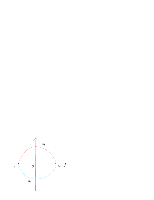
Figure 1. Existence of closed orbits for system (32).

We can illustrate the existence of a global center at the origin in Theorem 2 by taking $\varepsilon=0.1,b_{1}=2$, $c_{1}=0.6$, $d_{1}=-1$, $B_{1}=1$ and $C_{1}=-0.6$, as it is shown in Figure 2.

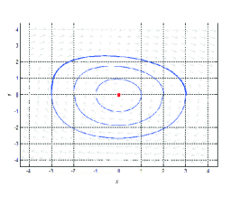
Figure 2. Existence of global center for system (32).

From the proof of statement (iii) in Theorem 2 and the averaging theory, we have the following results because $\tilde{f}_{41}(r)$ or $\tilde{f}_{42}(r)$ has at most two positive zeros.

Proposition 5.

At most $2$ limit cycles of system (9) can bifurcate from the periodic orbits of the linear system using the averaging theory of order four, and there are systems (9) with $2$ limit cycles.

References

[1]A. Andronov, A. Vitt and S. Khaikin,
Theory of Oscillations, Pergamon Press, Oxford, 1966.
[2]V.I. Arnold,
Loss of stability of self–oscillations close to resonance and
versal deformations of equivariant vector fields, Funct. Anal.
Appl. 11 (1977), 85–92.
[3]V.I. Arnold,
Ten problems, Adv. Soviet Math. 1 (1990), 1–8.
[4]M. di Bernardo, C.J. Budd, A.R. Champneys and P. Kowalczyk,
Piecewise-Smooth Dynamical Systems. Theory and Applications,
Appl. Math. Sci. Series, 163, Springer-Verlag London, Ltd., London,
2008.
[5]I.S. Berezin and N.P. Zhidkov,
Computing Methods, Volume II, Pergamon Press, Oxford, 1964.
[6]D.C. Braga and L.F. Mello,
Limit cycles in a family of discontinuous piecewise linear
differential systems with two zones in the plane, Nonlinear Dynam.
73 (2013), 1283–1288.
[7]C. Buzzi, C. Pessoa and J. Torregrosa,
Piecewise linear perturbations of a linear center, Discrete
and Continuous Dynamical Systems 33 (2013), 3915–3936.
[8]B. Coll,
Qualitative study of some vector fields in the plane (Thesis
in Catalan), Universitat Aut noma de Barcelona, 1987.
[9]F. Dumortier, J. Llibre and J. C. Artés,
Qualitative Theory of Planar Differential Systems,
Springer–Verlag, Berlin, 2006.
[10]E. Freire, E. Ponce, F. Rodrigo and F. Torres,
Bifurcation sets of continuous piecewise linear systems with
two zones, Internat. J. Bifur. Chaos Appl. Sci. Engrg. 8
(1998), 2073–2097.
[11]B. García, J. Llibre and J. S. Pérez del Río,
Planar quasihomogeneous polynomial differential systems and
their integrability, J. Differential Equation 255 (2013),
3185–3204.
[12]M. Han and W. Zhang,
On Hopf bifurcation in non-smooth planar systems, J.
Differential Equation 248 (2010), 2399–2416.
[13]S. Huan and X. Yang,
The number of limit cycles in general planar piecewise linear
systems, Discrete and Continuous Dynamical Systems 32
(2012), 2147–2164.
[14]J. Itikawa, J. Llibre and D.D. Novaes,
A new result on averaging theory for a class of discontinuous
planar differential systems with applications, to appear in Revista
Matemática Iberoamericana.
[15]A.G. Khovansky,
Real analytic manifolds with finiteness properties and complex
Abelian integrals, Funct. Anal. Appl. 18 (1984), 119–128.
[16]I.D. Iliev,
The number of limit cycles due to polynomial perturbations of
the harmonic oscillator, Math. Proc. Cambridge Philos. Soc. 127 (1999), 317–322.
[17]L. Li,
Three crossing limit cycles in planar piecewise linear systems
with saddle-focus type, Electron. J. Qual. Theory Differ. Equ.
2014, no. 70, pp. 14.
[18]J. Llibre, A.C. Mereu and D.D. Novaes,
Averaging theory for discontinuous piecewise differential
systems, J. Differential Equation 258 (2015), 4007–4032.
[19]J. Llibre, D.D. Novaes and M.A. Teixeira,
On the birth of limit cycles for non-smooth dynamical
systems, Bull. Sci. Math. 139 (2015) 229–244.
[20]J. Llibre and E. Ponce,
Three nested limit cycles in discontinuous piecewise linear
differential systems with two zones, Dynam. Contin. Discrete
Impuls. Systems. Ser. B Appl. Algorithms 19 (2011), 325–335.
[21]R. Lum and L.O. Chua,
Global properties of continuous piecewise-linear vector fields.
Part I: Simplest case in , Internat. J. Circuit Theory Appl.
19 (1991), 251–307.
[22]R. Lum and L.O. Chua,
Global properties of continuous piecewise–linear vector
fields. Part II: simplest symmetric in , Internat. J.
Circuit Theory Appl. 20 (1992), 9–46.
[23]O. Makarenkov and J.S.W. Lamb,
Dynamics and bifurcations of nonsmooth systems: A survey,
Physica D 241 (2012), 1826–1844.
[24]G. Sansone and R. Conti,
Non-Linear Differential Equations, 2nd edition,
Pergamon Press, New York, 1964.
[25]D. Schlomiuk and N. Vulpe,
Geometry of quadratic differential systems in the neighborhood
of infinity, J. Differential Equations 215 (2005), 357–400.
[26]D.J.W. Simpson,
Bifurcations in Piecewise–Smooth Continuous Systems, World
Scientific Series on Nonlinear Science A, vol 69, World
Scientific, Singapore, 2010.
[27]A.N. Varchenko,
An estimate of the number of zeros of an Abelian integral
depending on a parameter and limiting cycles, Funct. Anal. Appl.
18 (1984), 98–108.
[28]L. Wei and X. Zhang,
Limit cycle bifurcations near generalized homoclinic loop in
piecewise smooth differential systems, Discrete and Continuous
Dynamical Systems 36 (2016), 2803–2825.
[29]Y.Q. Ye,
Theory of Limit Cycles, Trans. Math. Monographs 66,
Amer. Math. Soc., Providence, RI, 1986.
[30]Y. Zou, T. Kupper and W.J. Beyn,
Generalized Hopf bifurcation for planar Filippov systems
continuous at the origin, J. Nonlinear Science 16 (2006), 159–177.