Thermophysical characteristics of the large main-belt asteroid (349) Dembowska

Abstract

(349) Dembowska, a large, bright main-belt asteroid, has a fast rotation and oblique spin axis. It may have experienced partial melting and differentiation. We constrain Dembowska’s thermophysical properties, e.g., thermal inertia, roughness fraction, geometric albedo and effective diameter within 3$\sigma$ uncertainty of $\Gamma=20^{+12}_{-7}\rm~{}Jm^{-2}s^{-0.5}K^{-1}$, $f_{\rm r}=0.25^{+0.60}_{-0.25}$, $p_{\rm v}=0.309^{+0.026}_{-0.038}$, and $D_{\rm eff}=155.8^{+7.5}_{-6.2}\rm~{}km$, by utilizing the Advanced Thermophysical Model (ATPM) to analyse four sets of thermal infrared data obtained by IRAS, AKARI, WISE and Subaru/COMICS at different epochs. In addition, by modeling the thermal lightcurve observed by WISE, we obtain the rotational phases of each dataset. These rotationally resolved data do not reveal significant variations of thermal inertia and roughness across the surface, indicating the surface of Dembowska should be covered by a dusty regolith layer with few rocks or boulders. Besides, the low thermal inertia of Dembowska show no significant difference with other asteroids larger than 100 km, indicating the dynamical lives of these large asteroids are long enough to make the surface to have sufficiently low thermal inertia. Furthermore, based on the derived surface thermophysical properties, as well as the known orbital and rotational parameters, we can simulate Dembowska’s surface and subsurface temperature throughout its orbital period. The surface temperature varies from $\sim 40$ K to $\sim 220$ K, showing significant seasonal variation, whereas the subsurface temperature achieves equilibrium temperature about $120\sim 160$ K below $30\sim 50$ cm depth.

1 Introduction

Asteroid (349) Dembowska was discovered on December 9, 1892. The asteroid locates in the main belt, orbiting around the Sun with a semi-major axis of 2.92 AU. The orbit of Dembowska is nearly circular, and show a prominent 7:3 resonance with Jupiter.

Dembowska was observed to be a bright asteroid with an absolute magnitude $H_{\rm v}\approx 5.93$, a phase slope parameter $G\approx 0.37$ (JPL, ; MPC, ). Thus Dembowska is believed to be a relatively large asteroid in the main belt. The effective diameter of Dembowska was derived to be $\sim$ $140~{}\rm km$ from the STM (Standard thermal model) fitting to IRAS data (Tedesco, 1989), indicating an unusually high geometric albedo about $0.38$.

Dembowska is classified to be the unique R-type asteroid, because its near infrared reflectance spectrum exhibits two strong absorption features at 1 and 2 $\mu m$, indicating an olivine-pyroxene mixture with little or no metal, where the pyroxene may be dominantly a calcium-poor and low iron ($\sim F_{s10-30}$) orthopyroxene like those in ordinary chondrites (Gaffey et al., 1993). Moreover, the Dembowska’s spectrum, reminiscent of (4) Vesta, suggests that the asteroid may have undergone partial melting or differentiation, making it a good target to study thermal melting and differentiation history of minor planets, where the accurate size, density, porosity and thermal state of Dembowska are required to serve as basic constraints on thermal differentiation models.

However, new observations of AKARI and WISE indicate the size of Dembowska could be much larger, and its albedo may not be so high as the previous reported value. Hanuš et al. (2013) showed the effective diameter of Dembowska derived from data detected by three space telescopes — IRAS, AKARI, and WISE, giving $D_{\rm IRAS}=139.8\pm 4.3~{}\rm km$, $D_{\rm AKARI}=164.7\pm 1.8~{}\rm km$ and $D_{\rm WISE}=216.7\pm 7.4~{}\rm km$, respectively. The derived sizes from different dataset significantly differ from each other, raising the question what the accurate size and albedo of Dembowska should be.

We note that the initial result of $D_{\rm IRAS}=139.8\pm 4.3~{}\rm km$ was obtained by the STM, whereas the update results of $D_{\rm AKARI}=164.7\pm 1.8~{}\rm km$ and $D_{\rm WISE}=216.7\pm 7.4~{}\rm km$ were derived by the NEATM (Harris, 1998). The various utilized models may lead to the difference in outcomes, while the difference between $D_{\rm AKARI}$ and $D_{\rm WISE}$ may mainly come from their different observation geometries, because WISE observed Dembowska nearly in an equatorial view, which has a larger cross-sectional area than the south region as observed by AKARI, according to Dembowska’s 3D shape model constructed by Torppa et al. (2003) with the light-curve inversion method developed by Kaasalainen & Torppa (2001). Therefore, to derive a more reliable and accurate size of the asteroid, we should adopt a more advanced thermophysical model to combine all available data together rather than use them separately.

On the other hand, Torppa et al. (2003) derived the rotation period of Dembowska to be about $4.701\rm~{}h$, indicating a faster rotation than many large main belt asteroids, and gave the orientation of rotation axis to be about $\lambda=150^{\circ}$, $\beta=+23^{\circ}$. Furthermore, Hanuš et al. (2013) updated the shape model of Dembowska, which looks like an asymmetrically elongated ellipsoid, and gave the best-fit spin axis orientation to be $\lambda=322^{\circ}$, $\beta=+18^{\circ}$. The spin axis nearly lies on the orbital plane, which could cause significant seasonal variation of surface temperature on high local latitudes, and thus play a role in the thermophysical properties of the surface materials. In the present work, we implement the radiometric method, where the Advanced thermophysical modelling (ATPM) algorithm (Rozitis & Green, 2011; Yu, Ji & Wang, 2014; Yu & Ji, 2015; Yu, Ji & Ip, 2017) is used to analyse four independent mid-infrared datasets (IRAS, WISE, AKARI and Subaru) of (349) Dembowska, where the details of the data source are provided in section 2.1. With the radiometric method, the size of Dembowska, as well as the surface thermal inertia, roughness fraction and geometric albedo are well determined in section 3. In addition, in section 4, based on the derived surface properties, we investigate the surface and subsurface thermal state of Dembowska, which show significant seasonal variations.

2 Radiometric Procedure

2.1 Thermal infrared Observations

In this work, we use the thermal infrared data provided by the IRAS, AKARI satellite, and the WISE space telescope as well as a new dataset observed by the Subaru telescope atop Mauna Kea.

The Subaru observations were carried out on UT January 18, 2014, using the Cooled MIR Camera and Spectrometer (COMICS; Kataza et al., 2000) on the 8.2 m Subaru Telescope. We adopted the N7.8, N8.7, N9.8, N10.3, N11.6, N12.5 continuum filters in the N-band and the Q18.8 and Q24.5 filters in the Q-band. Immediately before and/or after the observations of the target, we observed a nearby flux standard star selected from Cohen et al. (1999). Data reduction followed the procedures described in the Subaru Data Reduction CookBook: COMICS, prepared by Y. Okamoto and the COMICS team.

The IRAS data were obtained from the IMPS Sightings Data Base of VizieR. The AKARI data were provided by F. Usui (private comm.). The WISE data are obtained from the WISE archive. We convert the magnitude data to flux with color corrections (W3:1.0006; W4:0.9833). The derived monochromatic flux densities for the W3 and W4 band observations have an associated uncertainty of $\pm 10$ percent (Wright et al., 2010).

All these data are utilized in this work to be compared with the theoretical flux simulated from the Advanced thermophysical Model (ATPM) so as to derive the possible scale of surface thermophysical properties. We tabulate all the utilized data in Table 1.

Table 1: Mid-infrared observations of 349 Dembowska.

UT	Flux (Jy)				$r_{\rm helio}$	$\Delta_{\rm obs}$	$\alpha$	Observatory
	12.0 ($\mu m$)	25.0 ($\mu m$)	65.0 ($\mu m$)	100.0 ($\mu m$)	(AU)	(AU)	(∘)	Instrument
1983-02-17 07:03	6.47$\pm$0.64	19.13$\pm$2.77	8.91$\pm$1.94	2.87$\pm$0.58	2.809	2.480	-20.32	IRAS
1983-02-17 08:46	7.47$\pm$0.81	20.87$\pm$2.75	10.03$\pm$2.19	3.10$\pm$0.67	2.809	2.481	-20.33	IRAS
1983-02-17 10:29	6.81$\pm$0.68	19.16$\pm$2.46	11.71$\pm$2.81	2.61$\pm$0.52	2.809	2.482	-20.33	IRAS
1983-03-02 06:01	5.69$\pm$0.65	16.88$\pm$2.24	9.08$\pm$2.21	2.75$\pm$0.55	2.820	2.666	-20.56	IRAS
1983-03-02 07:44	5.92$\pm$0.59	16.06$\pm$2.62	8.85$\pm$2.14	3.61$\pm$0.79	2.820	2.667	-20.56	IRAS
1983-03-02 09:27	7.46$\pm$0.74	19.96$\pm$2.68	11.56$\pm$2.58	3.67$\pm$0.75	2.820	2.668	-20.56	IRAS
UT	Wavelength		Flux		$r_{\rm helio}$	$\Delta_{\rm obs}$	$\alpha$	Observatory
	($\mu m$)		(Jy)		(AU)	(AU)	(∘)	Instrument
2006-05-11 01:52	18.0		19.08$\pm$1.27		2.858	2.684	20.68	AKARI
2006-05-11 03:31	18.0		19.05$\pm$1.27		2.858	2.684	20.68	AKARI
2006-05-11 11:46	9.0		3.54$\pm$0.21		2.858	2.679	20.69	AKARI
2006-05-11 13:25	9.0		3.58$\pm$0.22		2.858	2.678	20.69	AKARI
2006-05-11 15:05	9.0		3.40$\pm$0.22		2.858	2.677	20.69	AKARI
2006-11-11 20:57	18.0		20.93$\pm$1.40		2.719	2.541	-21.34	AKARI
2006-11-11 22:37	18.0		21.43$\pm$1.43		2.719	2.541	-21.34	AKARI
2006-11-12 00:16	18.0		21.17$\pm$1.41		2.719	2.543	-21.34	AKARI
UT	Flux (Jy)				$r_{\rm helio}$	$\Delta_{\rm obs}$	$\alpha$	Observatory
	11.0 ($\mu m$)		22.0 ($\mu m$)		(AU)	(AU)	(∘)	Instrument
2010-02-14 12:45	2.39$\pm$0.24		7.78$\pm$0.78		3.170	3.010	18.15	WISE
2010-02-14 12:46	2.39$\pm$0.24		7.78$\pm$0.78		3.170	3.010	18.15	WISE
2010-02-14 22:17	2.54$\pm$0.25		8.47$\pm$0.85		3.170	3.004	18.15	WISE
2010-02-14 23:52	2.60$\pm$0.26		8.29$\pm$0.82		3.169	3.003	18.15	WISE
2010-02-15 01:28	3.65$\pm$0.36		11.07$\pm$1.11		3.169	3.002	18.15	WISE
2010-02-15 03:03	2.65$\pm$0.26		8.48$\pm$0.84		3.169	3.001	18.15	WISE
2010-02-15 12:35	3.09$\pm$0.31		9.81$\pm$0.98		3.169	2.996	18.15	WISE
2010-02-15 15:45	3.44$\pm$0.34		9.95$\pm$0.99		3.169	2.994	18.15	WISE
2010-08-04 02:37	3.37$\pm$0.33		10.82$\pm$1.08		3.090	2.822	-19.07	WISE
2010-08-04 05:47	3.04$\pm$0.30		9.94$\pm$0.99		3.090	2.823	-19.07	WISE
2010-08-04 08:58	4.65$\pm$0.46		12.64$\pm$1.26		3.090	2.825	-19.08	WISE
2010-08-04 12:08	3.11$\pm$0.31		9.78$\pm$0.98		3.090	2.827	-19.08	WISE
2010-08-04 13:43	4.45$\pm$0.44		12.95$\pm$1.29		3.090	2.828	-19.08	WISE
2010-08-04 15:19	2.82$\pm$0.28		9.46$\pm$0.94		3.089	2.829	-19.08	WISE
2010-08-04 16:54	3.49$\pm$0.34		10.16$\pm$1.01		3.089	2.830	-19.08	WISE
2010-08-04 23:15	4.07$\pm$0.41		11.90$\pm$1.19		3.089	2.833	-19.09	WISE
2010-08-05 02:25	2.97$\pm$0.30		9.40$\pm$0.94		3.089	2.835	-19.09	WISE
2010-08-05 05:36	2.88$\pm$0.29		9.69$\pm$0.97		3.089	2.836	-19.10	WISE
UT	Wavelength		Flux		$r_{\rm helio}$	$\Delta_{\rm obs}$	$\alpha$	Observatory
	($\mu m$)		(Jy)		(AU)	(AU)	(∘)
2014-01-18 12:39	7.8		2.85$\pm$0.45		3.086	2.337	13.63	Subaru
2014-01-18 12:43	8.7		3.84$\pm$0.47		3.086	2.337	13.63	Subaru
2014-01-18 12:47	9.8		6.02$\pm$0.72		3.086	2.337	13.63	Subaru
2014-01-18 12:51	10.3		8.10$\pm$0.94		3.086	2.337	13.63	Subaru
2014-01-18 12:54	11.6		11.11$\pm$1.26		3.086	2.337	13.63	Subaru
2014-01-18 12:58	12.5		12.44$\pm$1.42		3.086	2.337	13.63	Subaru
2014-01-18 13:04	18.7		21.74$\pm$2.71		3.086	2.337	13.63	Subaru
2014-01-18 13:10	24.5		25.82$\pm$5.57		3.086	2.337	13.63	Subaru

2.2 Advanced thermophysical model

The Advanced thermophysical model reproduces the thermal state and thermal emission of an asteroid by solving 1D thermal conduction in consideration of roughness, where the asteroid is described by a polyhedron composed of $N$ triangle facets, and the roughness is modelled by a fractional coverage of hemispherical macroscopic craters, symbolized by $f_{\rm r}$ ($0\leq f_{\rm r}\leq 1$), while the remaining fraction, $1-f_{\rm r}$, represents smooth flat surface ($f_{\rm r}=0$ means the whole surface is smooth flat).

For such rough surface facets, the conservation of energy leads to an instant heat balance between sunlight, multiple-scattered sunlight, thermal emission, thermal-radiated fluxes from other facets and heat conduction. If the asteroid keeps a periodical rotation, the temperature $T_{i}$ and thermal emission $B_{i}$ of facet $i$ will change periodically as well. Therefore, we can build numerical codes to simulate $T_{i}$ and $B_{i}$ at any rotation phase for the asteroid. For a given observation epoch, ATPM can reproduce a theoretical profile to each observation flux as:

$$F_{\rm model}(\lambda)=\sum^{N}_{i=1}\epsilon(\lambda)\pi B(\lambda,T_{i})S(i)f(i)~{},$$ (1)

where $\epsilon(\lambda)$ is the monochromatic emissivity at wavelength $\lambda$, $S(i)$ is the area of facet $i$, $f(i)$ is the view factor of facet $i$ to the telescope

$$f(i)=v_{i}\frac{\vec{n}_{i}\cdot\vec{n}_{\rm obs}}{\pi\Delta^{2}},~{}$$ (2)

$v_{\rm i}$ indicates visible fraction of facet $i$, and $B(\lambda,T_{i})$ is the Planck intensity function:

$$B(\lambda,T_{i})=\frac{2hc^{2}}{\lambda^{5}}\frac{1}{\exp\big{(}\frac{hc}{\lambda kT_{i}}\big{)}-1}~{}.$$ (3)

Thus the calculated $F_{\rm model}$ can be compared with the thermal infrared fluxes summarized in Table 1 in the fitting process.

2.3 Fitting Procedure

In order to reproduce thermal state and thermal emission of an asteroid via the ATPM procedure, several input physical parameters are needed, including the 3D shape model, effective diameter $D_{\rm eff}$, bond albedo, and the so-called thermal parameter

$$\Phi=\frac{\Gamma\sqrt{\omega}}{\varepsilon\sigma T^{3}_{\rm eff}}~{},$$ (4)

where $\omega$ is the rotation frequency, $\Gamma$ is the thermal inertia, $\varepsilon$ is the averaged thermal emissivity over the entire emission spectrum, and

$$T_{\rm eff}=\left[\frac{(1-A_{\rm B})F_{\odot}}{\varepsilon\sigma d_{\rm\odot}^{2}}\right]^{1/4}~{},$$

is the effective temperature. The rotation frequency $\omega$ can be determined from light curves, while thermal inertia $\Gamma$ is the parameter of interest which would be treated as free parameter in the fitting procedure.

Figure 1 shows the 3D shape model of 349 Dembowska published in the Database of Asteroid Models from Inversion Techniques (DAMIT). This shape model is updated by Hanuš et al. (2013) according to the light-curve inversion method developed by Kaasalainen & Torppa (2001). We utilize this shape model in our thermophysical modelling procedure.

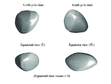
Figure 1: The shape model of 349 Dembowska downloaded from DAMIT (Database of Asteroid Models from Inversion Techniques).

According to Fowler & Chillemi (1992), an asteroid’s effective diameter $D_{\rm eff}$, defined by the diameter of a sphere with a identical volume to that of the shape model, can be related to its geometric albedo $p_{v}$ and absolute visual magnitude $H_{v}$ via:

$$D_{\rm eff}=\frac{1329\times 10^{-H_{v}/5}}{\sqrt{p_{v}}}~{}(\rm km)~{}.$$ (5)

In addition, the geometric albedo $p_{v}$ is related to the effective Bond albedo $A_{\rm eff,B}$ by

$$A_{\rm eff,B}=p_{v}q_{\rm ph}~{},$$ (6)

where $q_{\rm ph}$ is the phase integral that can be approximated by

$$q_{\rm ph}=0.290+0.684G~{},$$ (7)

in which $G$ is the slope parameter in the $H,G$ magnitude system of Bowell et al. (1989). We obtain $H_{\rm v}=5.93,G=0.37$ from the JPL Website ($https://ssd.jpl.nasa.gov/sbdb.cgi\#top$).

On the other hand, the asteroid’s effective Bond albedo is the averaged result of both the albedo of smooth and rough surface, which can be expressed as the following relationship:

$$A_{\rm eff,B}=(1-f_{\rm r})A_{B}+f_{\rm r}\frac{A_{B}}{2-A_{B}}~{},$$ (8)

where $A_{B}$ is the Bond albedo of smooth lambertian surface. Thus an input roughness fraction $f_{\rm r}$ and geometric albedo $p_{\rm v}$ can lead to an unique Bond albedo $A_{B}$ and effective diameter $D_{\rm eff}$ to be used to fit the observations.

Then we actually have three free parameters — thermal inertia, roughness fraction, and geometric albedo (or effective diameter) that would be extensively investigated in the fitting process. We use the so-called reduced $\chi^{2}_{\rm r}$ defined as

$$\chi^{2}_{\rm r}=\frac{1}{n-3}\sum^{n}_{i=1}\Big{[}\frac{F_{\rm model}(\lambda_{i},\Gamma,f_{\rm r},p_{\rm v})-F_{\rm obs}(\lambda_{i})}{\sigma_{\lambda_{i}}}\Big{]}^{2}~{},$$ (9)

to assess the fitting degree of our model with respect to the observations. Other parameters are listed in Table 2.

Table 2: Assumed physical parameters used in ATPM.

Property	Value	References
Number of vertices	1022	(Hanuš et al., 2013)
Number of facets	2040	(Hanuš et al., 2013)
Shape (a:b:c)	1.4165:1.2569:1	(Hanuš et al., 2013)
Spin axis	($322.0^{\circ}$,$18.0^{\circ}$)	(Hanuš et al., 2013)
Spin period	4.701 h	(Torppa et al., 2003)
Absolute magnitude	5.93	(JPL, ; MPC, )
Slope parameter	0.37	(JPL, ; MPC, )
Emissivity $\varepsilon$	0.9	Assumed
Emissivity $\epsilon(\lambda)$	0.9	Assumed

3 Analysis and Results

3.1 Fitting with rotationally averaged flux

Due to the uncertainties of rotation phases at different observation epochs, we choose rotationally averaged model flux $F_{\rm model}$ to fit the observations. Thus the investigated thermophysical parameters would be averaged profiles across the whole surface. Table 3 lists the reduced $\chi^{2}_{\rm r}$ derived from each input parameters, where we scan the thermal inertia in the range of $0\sim 50\rm~{}Jm^{-2}s^{-0.5}K^{-1}$ and roughness fraction $0\sim 1.0$, while for each pair of thermal inertia and roughness fraction, the geometric albedo giving the minimum reduced $\chi^{2}_{\rm r}$ is found.

Table 3: ATPM fitting results to the observations.

Roughness	Thermal inertia $\Gamma$ ($\rm~{}Jm^{-2}s^{-0.5}K^{-1}$)
fraction	5		10		15		20		25		30		35		40		45
$f_{\rm R}$	$p_{\rm v}$	$\chi^{2}_{\rm r}$	$p_{\rm v}$	$\chi^{2}_{\rm r}$	$p_{\rm v}$	$\chi^{2}_{\rm r}$	$p_{\rm v}$	$\chi^{2}_{\rm r}$	$p_{\rm v}$	$\chi^{2}_{\rm r}$	$p_{\rm v}$	$\chi^{2}_{\rm r}$	$p_{\rm v}$	$\chi^{2}_{\rm r}$	$p_{\rm v}$	$\chi^{2}_{\rm r}$	$p_{\rm v}$	$\chi^{2}_{\rm r}$
0.00	0.325	2.572	0.310	2.199	0.297	1.989	0.287	1.908	0.278	1.931	0.271	2.035	0.264	2.201	0.258	2.415	0.254	2.664
0.05	0.328	2.604	0.315	2.201	0.304	1.974	0.295	1.885	0.287	1.906	0.280	2.012	0.274	2.183	0.269	2.404	0.264	2.661
0.10	0.333	2.642	0.319	2.209	0.308	1.966	0.298	1.868	0.290	1.887	0.283	1.995	0.277	2.171	0.272	2.399	0.267	2.664
0.15	0.338	2.685	0.324	2.224	0.312	1.963	0.302	1.857	0.294	1.874	0.286	1.984	0.280	2.165	0.275	2.399	0.270	2.672
0.20	0.343	2.732	0.328	2.243	0.316	1.966	0.306	1.852	0.297	1.865	0.290	1.978	0.283	2.163	0.278	2.404	0.273	2.685
0.25	0.347	2.783	0.332	2.267	0.320	1.974	0.309	1.851	0.300	1.862	0.293	1.976	0.286	2.166	0.280	2.413	0.275	2.701
0.30	0.352	2.837	0.336	2.294	0.323	1.985	0.312	1.854	0.303	1.863	0.295	1.978	0.289	2.173	0.283	2.426	0.278	2.721
0.35	0.356	2.893	0.340	2.324	0.327	2.000	0.315	1.861	0.306	1.867	0.298	1.984	0.291	2.183	0.285	2.442	0.280	2.745
0.40	0.360	2.951	0.343	2.357	0.330	2.017	0.318	1.871	0.309	1.875	0.301	1.994	0.294	2.197	0.288	2.462	0.282	2.771
0.45	0.364	3.011	0.347	2.393	0.333	2.038	0.321	1.884	0.311	1.886	0.303	2.006	0.296	2.213	0.290	2.484	0.284	2.801
0.50	0.367	3.072	0.350	2.430	0.336	2.061	0.324	1.900	0.314	1.899	0.305	2.021	0.298	2.232	0.292	2.509	0.286	2.832
0.55	0.370	3.135	0.353	2.469	0.338	2.086	0.326	1.918	0.316	1.915	0.307	2.039	0.300	2.254	0.294	2.536	0.288	2.866
0.60	0.373	3.197	0.355	2.509	0.341	2.113	0.328	1.938	0.318	1.933	0.309	2.058	0.302	2.277	0.295	2.565	0.290	2.901
0.65	0.376	3.260	0.358	2.551	0.343	2.141	0.330	1.960	0.320	1.953	0.311	2.079	0.304	2.303	0.297	2.596	0.291	2.939
0.70	0.379	3.324	0.360	2.593	0.345	2.171	0.332	1.983	0.322	1.975	0.313	2.103	0.305	2.330	0.298	2.628	0.293	2.977
0.75	0.381	3.387	0.362	2.637	0.347	2.202	0.334	2.008	0.323	1.998	0.314	2.127	0.306	2.358	0.300	2.662	0.294	3.017
0.80	0.383	3.451	0.364	2.681	0.348	2.234	0.335	2.034	0.324	2.022	0.315	2.153	0.307	2.388	0.301	2.697	0.295	3.059
0.85	0.385	3.514	0.365	2.725	0.350	2.268	0.336	2.061	0.326	2.048	0.316	2.181	0.308	2.419	0.302	2.733	0.296	3.101
0.90	0.386	3.577	0.366	2.770	0.351	2.301	0.337	2.089	0.326	2.075	0.317	2.209	0.309	2.451	0.302	2.771	0.297	3.145
0.95	0.387	3.640	0.367	2.815	0.352	2.335	0.338	2.118	0.327	2.102	0.318	2.238	0.310	2.484	0.303	2.809	0.297	3.188
1.00	0.424	3.702	0.393	2.860	0.369	2.370	0.350	2.147	0.334	2.130	0.321	2.269	0.310	2.518	0.301	2.848	0.293	3.233

According to Table 3, we can see that a low thermal inertia between $20\sim 30\rm~{}Jm^{-2}s^{-0.5}K^{-1}$ tends to fit better to the observations; the minimum reduced $\chi^{2}_{\rm r}$ arises around the case of $p_{\rm v}=0.309$, $f_{\rm r}=0.25$, and $\Gamma=20$$\rm~{}Jm^{-2}s^{-0.5}K^{-1}$, which can be adopted as the best solution for the geometric albedo, thermal inertia and roughness fraction of Dembowska.

Figure 2 shows the contour of $\chi^{2}_{\rm r}(\Gamma,f_{\rm r})$ based on the results listed in Table 3, where the values of $\chi^{2}_{\rm r}$ are represented by colour and the variation of ColorBar from blue to red means the increase of $\chi^{2}_{\rm r}$. The black ’+’ shows the location of minimum $\chi^{2}_{\rm r}$ in the ($\Gamma$, $f_{\rm r}$) parameter space. The blue curve labeled by 1$\sigma$ corresponding to $\Delta\chi^{2}_{\rm r}=3.52/(76-3)=0.0482$ from the minimum $\chi^{2}_{\rm r}$, which constrains the range of free parameters $\Gamma=20^{+6}_{-3}\rm~{}Jm^{-2}s^{-0.5}K^{-1}$, $f_{\rm r}=0\sim 0.5$, with probability of $68.3\%$, while the cyan curve labeled by 3$\sigma$ refers to $\Delta\chi^{2}_{\rm r}=14.2/(76-3)=0.1945$, giving the range of free parameters $\Gamma=20^{+12}_{-7}\rm~{}Jm^{-2}s^{-0.5}K^{-1}$, $f_{\rm r}=0\sim 0.85$ with probability of $99.73\%$ (Press et al., 2007).

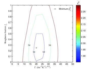
Figure 2: $\chi^{2}_{\rm r}$ ($f_{\rm r}$, $\Gamma$) contour according to Table 3. The color (from blue to red) means the increase of profile of $\chi^{2}_{\rm r}$. The 1$\sigma$ boundary corresponds to $\Delta\chi^{2}_{\rm r}=3.52/(76-3)=0.0482$, while the 3$\sigma$ boundary corresponds to $\Delta\chi^{2}_{\rm r}=14.2/(76-3)=0.1945$ (Press et al., 2007).

In consideration of the above derived 1$\sigma$ and 3$\sigma$ range of thermal inertia $\Gamma$ and roughness fraction $f_{\rm r}$, the corresponding geometric albedo $p_{\rm v}$ and $\chi^{2}_{\rm r}$ are selected out, yielding the $p_{\rm v}\sim\chi^{2}_{\rm r}$ relation showed in Figure 3. Then the 1$\sigma$ scale of geometric albedo can be constrained to be $p_{\rm v}=0.309^{+0.012}_{-0.019}$, while the 3$\sigma$ scale is $p_{\rm v}=0.309^{+0.026}_{-0.038}$.

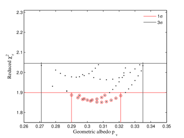
Figure 3: $p_{\rm v}\sim\chi^{2}_{\rm reduced}$ profiles fit to the observations in consideration of all $f_{\rm r}$ and $\Gamma$ in the derived 1$\sigma$ and 3$\sigma$ range.

To verify the the reliability of the above fitting procedure and derived outcomes, we employ the ratio of ’observation/model’ to examine how these theoretical model results match the observations at various observation wavelengths and observation geometries (see Figure 4 and 5), because these factors are the basic variables of the observations.

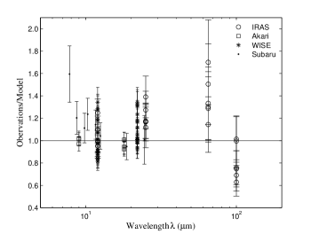
Figure 4: The observation/model ratios as a function of wavelength for $\Gamma=20\rm~{}Jm^{-2}s^{-0.5}K^{-1}$, $f_{\rm r}=0.25$, $p_{\rm v}=0.309$ and $D_{\rm eff}=155.8\rm~{}km$.

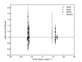
Figure 5: The observation/model ratios as a function of solar phase angle for $\Gamma=20\rm~{}Jm^{-2}s^{-0.5}K^{-1}$, $f_{\rm r}=0.25$, $p_{\rm v}=0.309$ and $D_{\rm eff}=155.8\rm~{}km$.

In Figure 4, the observation/Model ratios are shown at each observational wavelength for $\Gamma=20\rm~{}Jm^{-2}s^{-0.5}K^{-1}$, $f_{\rm r}=0.25$, $p_{\rm v}=0.309$ and $D_{\rm eff}=155.8\rm~{}km$. The ratios are evenly distributed around 1.0 without significant wavelength dependent features, despite the ratio at $7.8\rm~{}\mu m$ moves relatively farther from unity. In Figure 5, we show how the model results match observations at each observational solar phase angle, where the ratios are all nearly symmetrical distributed around 1.0 and no phase-angle dependent features exit as well. Thus the relatively large deviation for the $7.8\rm~{}\mu m$ data observed by Subaru may be caused by large observation uncertainty. We note that ground-based observations are vulnerable to telluric absorptions. The atmosphere at $7.8\rm~{}\mu m$ is only about $60-80\%$ transparent, therefore it is expected that the uncertainty of the flux measurement at this band is relatively higher than other wavelengths. The telluric contamination explains the relatively large deviation of the $7.8\rm~{}\mu m$ data from the model. Nevertheless, the fitting procedure is reliable, but more accurate data especially that observed at low phase angle and at wavelength around Wien peak are needed to examine our results. We summarize all the derived results from the above thermophysical modelling process in Table 4.

Table 4: Derived Results from rotationally averaged fitting.

Properties	$1\sigma$ value	$3\sigma$ value
Thermal inertia $\Gamma$($\rm~{}Jm^{-2}s^{-0.5}K^{-1}$)	$20^{+6}_{-3}$	$20^{+12}_{-7}$
Roughness fraction $f_{\rm r}$	$0\sim 0.5$	$0\sim 0.85$
Geometric albedo $p_{\rm v}$	$0.309^{+0.012}_{-0.019}$	$0.309^{+0.026}_{-0.038}$
Effective diameter $D_{\rm eff}$ (km)	$155.8^{+5.0}_{-3.0}$	$155.8^{+7.5}_{-6.2}$

3.2 Fitting with thermal light curve

Since the IRAS and WISE data do not cover an entire rotation period and were observed at various solar phase angles, they cannot be used to generate thermal light curves directly. However, Dembowska is a large and well-observed asteroid with known orbital and rotational parameters, thus in principle, we could derive the rotational phase of each observation data with respect to a defined local body-fixed coordinate system if we know the observed rotational phase at a particular epoch, then these data can be used to create thermal light curves.

We use the published 3D shape model of Dembowska showed in Figure 1 to define the local body-fixed coordinate system, where the z-axis is chosen to be the rotation axis, and ”zero” rotational phase is chosen to be the ”Equatorial view ($0^{\circ}$)” in Figure 1. Moreover, if we define the view angle of one observation with respect to the body-fixed coordinate system to be $(\varphi,\theta)$, where $\varphi$ stands for local longitude, and $\theta$ means local latitude, then the rotational phase $ph$ of this observation can be related to the local longitude $\varphi$ via

$$ph=1-\varphi/(2\pi).$$ (10)

If assuming the rotational phase at epoch 2010-02-14 12:45 to be $zph$, then all the rotational phases of other data could be derived in consideration of the observation time and geometry. However, the observation time of the IRAS data deviate so long away from the reference epoch 2010-02-14 12:45 that even tiny uncertainty of rotation period can accumulate significant estimation errors of the rotational phases. Thus we only fit the rotationally resolved flux data of WISE so as to find out which $zph$ can fit the data best. Of course, other parameters mentioned above are necessary. Since the surface thermal inertia, albedo and size are well constrained within 3$\sigma$ by the above rotationally averaged fitting, we could use the derived best-fit profiles as definite parameters. But for the roughness fraction, the uncertainty is relatively larger. Therefore we use $f_{\rm r}$ and $zph$ together as free parameters to fit the WISE data, and the results are showed in Figure 6.

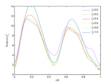
Figure 6: Horizontal axis: $zph$ represents the observed rotational phase of Dembowska at epoch 2010-02-14 12:45. Vertical axis: obtained reduced $\chi^{2}_{\rm r}$ with different input $zph$ and roughness fraction $f_{\rm r}$. The curves in different color stand for different $f_{\rm r}$ ranging from $0.0\sim 1.0$.

Figure 6 shows how different $zph$ and roughness fraction $f_{\rm r}$ match the observations, where $zph=0.98$ and $f_{\rm r}\sim 0.4$ (shown by the black ’+’ in Figure 6) seem to achieve best degree of fitting. Thus we adopt $zph=0.98$ as the rotational phase of Dembowska at epoch 2010-02-14 12:45, and use it to derive the rotational phases of other data. With the derived rotational phases, we are able to convert the WISE data into one rotation period, and make comparisons with the modeled thermal light curve, as showed in Figure 7, where the colorized curves are the modeled thermal light curves with the above best-fit results of $\Gamma=20\rm~{}Jm^{-2}s^{-0.5}K^{-1}$, $p_{\rm v}=0.309$, $D_{\rm eff}=155.8\rm~{}km$, and two different roughness fraction cases $f_{\rm r}=0.0,0.4$. The difference between the blue and red curves are caused by different heliocentric and observation distance at each epoch. Figure 7 shows that the modeled curves with higher roughness fraction $f_{\rm r}\approx 0.4$ tends to better match the observations.

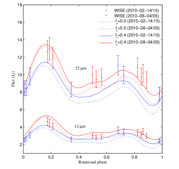
Figure 7: Thermal light curve of Dembowska. The blue data corresponds to epoch 2010-02-14 12:45, the red data corresponds to epoch 2010-08-04 02:37; the colorized curves are modeled with $\Gamma=20\rm~{}Jm^{-2}s^{-0.5}K^{-1}$, $p_{\rm v}=0.309$, $D_{\rm eff}=155.8\rm~{}km$, while the dashed curves refer to modeled curves with input roughness fraction $f_{\rm r}=0.0$, and the solid curves refer to $f_{\rm r}=0.4$.

It should be noticed here that the observations differ from each other not only in rotational phase, but also in view angle. With the above determined rotational phases, we can derive the exact view angle of each observation with respect to the defined local body-fixed coordinate system, and show them in Figure 8, which exhibits that IRAS and WISE observed Dembowska nearly in equatorial region, whereas AKARI observed south region and Subaru observed north region.

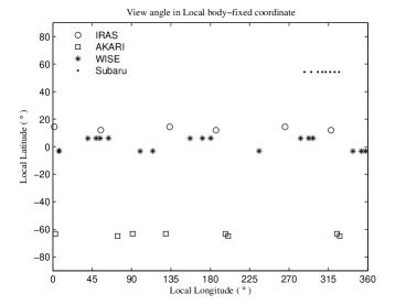
Figure 8: View angles of each observation with respect to the defined local body-fixed coordinate system.

We could investigate whether heterogeneous feature of surface thermophysical properties appear along local longitude by checking how the observation/Model ratios of WISE data vary with rotational phase in Figure 9, where the modeled fluxes are obtained by ATPM with the above determined best-fit parameters $f_{\rm r}=0.4$, $\Gamma=20\rm~{}Jm^{-2}s^{-0.5}K^{-1}$, $p_{\rm v}=0.309$ and $D_{\rm eff}=155.8\rm~{}km$. The ratios are distributed nearly around 1.0 without significant rotational phase dependent features, despite a slight increasing tendency from rotational phase $0.2$ to $0.8$, which may indicate heterogeneous surface properties between the West and East part of Dembowska. But this kind of heterogeneous signal is rather weak to further infer variation of surface properties along local longitude in consideration of observation uncertainties. On the other hand, Figure 10 shows the observation/Model ratios corresponding to different view latitudes, where the ratios tend to be $<1.0$ for south region but $>1.0$ for north region, indicating a slight heterogeneous feature between the south and north region of Dembowska. However, the heterogeneous signal is also very week due to the relatively large observational uncertainties. Thus we may surmise that no significant large variation of surface thermophysical characteristics appear over the surface of Dembowska.

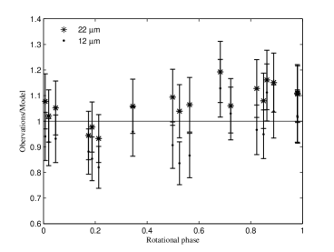
Figure 9: The observation/model ratios as a function of rotational phase in equatorial view for $f_{\rm r}=0.4$, $\Gamma=20\rm~{}Jm^{-2}s^{-0.5}K^{-1}$, $p_{\rm v}=0.309$ and $D_{\rm eff}=155.8\rm~{}km$.

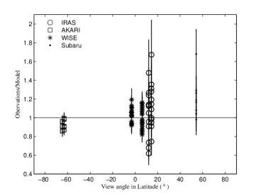
Figure 10: The observation/model ratios as a function of view angle in local latitude for $f_{\rm r}=0.4$, $\Gamma=20\rm~{}Jm^{-2}s^{-0.5}K^{-1}$, $p_{\rm v}=0.309$ and $D_{\rm eff}=155.8\rm~{}km$.

4 Surface Thermal State

In this section, we use the above derived surface thermophysical properties to further investigate the surface and subsurface thermal environment of Dembowska based on its present rotational and orbital motion state. In consideration of the large axial tilt between the rotational axis and orbital axis, it can be imagined that interesting seasonal variation of temperature would appear on the surface of Dembowska, which may have potential influence both on the thermophysical and spectral properties of the surface materials.

Temperature variation can be caused by both orbital motion and rotation. Thus, to figure out the seasonal variation of temperature, we have to remove the diurnal effect caused by rotation, where a ’diurnal averaged temperature’ is needed. The so-called diurnal averaged temperature can be obtained by solving the 1D thermal conduction equation with a rotationally averaged energy conservation condition as

$$(1-A_{\rm eff})\tilde{F}_{\rm s}=\varepsilon\sigma\tilde{T}^{4}-\kappa\frac{\delta\tilde{T}}{\delta h}~{},$$ (11)

where $h$ means depth, $A_{\rm eff}$ is effective bond albedo derived from geometric albedo, $\kappa$ is the thermal conductivity estimated from the above derived thermal inertia, $\tilde{T}$ is the diurnal averaged temperature of interest, and $\tilde{F}_{\rm s}$ refers to the diurnal averaged incident solar flux given by

$$\tilde{F}_{\rm s}=\frac{F_{\odot}}{r_{\odot}^{2}}\frac{1}{2\pi}\int^{2\pi}_{0}\max(0,\vec{n}_{\odot}\cdot\vec{n}_{i}(\theta,\varphi)){\rm d}\varphi,$$ (12)

in which $r_{\odot}$ is the heliocentric distance, $F_{\odot}$ is the solar constant $1361.5\rm~{}Wm^{-2}$, $\vec{n}_{\odot}$ means the direction pointing to the Sun, $\vec{n}_{i}(\theta,\varphi)$ is the normal vector of facet $i$ at the local latitude $\theta$ and longitude $\varphi$.

In Figure 11, the upper panel shows the diurnal averaged incident solar flux $\tilde{F}_{\rm s}$ on each latitude of Dembowska at different orbital position, while the under panel shows the corresponding diurnal averaged temperature. We can see that within an orbital period, the temperature changes smoothly at equator, but shows large variations at high latitudes, where even appear polar night and polar day at around mean anomaly$=-60^{\circ}$ and $=120^{\circ}$. Besides, at each orbital position, the temperature of Dembowska’s south and north region shows large difference, which changes periodically following the orbital period. Thus it is reasonable to infer that the thermophysical and spectral properties of the south and north region may be different at different orbital position.

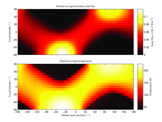
Figure 11: Upper panel: the diurnal averaged incident solar flux $\tilde{F}_{\rm s}$; Under panel: the diurnal averaged temperature; horizontal axis stands for mean anomaly, where $0$ means the perihelion; vertical axis stands for local latitude on Dembowska, where $0$ means the equator and positive means north, negative means south. The surface temperature at each latitude shows significant seasonal variation, which may affect the surface properties of Dembowska.

Figure 12 further shows how temperature varies in an orbital period at equator, north and south region of Dembowska respectively. We can see that the diurnal averaged temperature at equator can fluctuate within $140\sim 180$ K, while the temperatures at north and south vary from minimum temperature $\sim 40$ K to maximum temperature $\sim 220$ K. And, particular near anomaly$=-60^{\circ}$ and $=120^{\circ}$, the temperature difference between the south pole and north pole can be as large as $\sim 180$ K, which could cause different thermophysical or spectral characteristics.

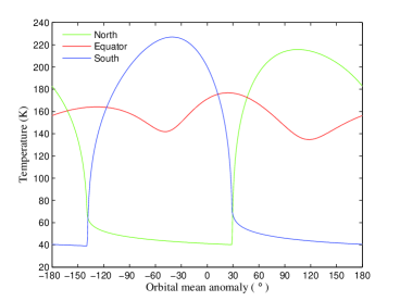
Figure 12: Seasonal variation of the diurnal averaged temperature at equator, north and south region of Dembowska respectively.

Figure 13 shows the temperature distribution within the subsurface of Dembowska’s equator, north, and south region. The curves labeled by red, green, and blue stands for equator, north and south respectively. The different curves plotted in the same color represents the temperature distribution at different orbital position in a whole orbit period. The subsurface temperature on the equator could achieve equilibrium $\sim 160$ K at about $30$ cm below the surface, while on the north and south region, the equilibrium subsurface temperature appear to be $\sim 120$ K at about $50$ cm depth. Therefore, it is possible for us to further investigate the subsurface properties by detecting the microwave emission of Dembowska at wavelength around $3\sim 5$ cm.

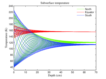
Figure 13: Seasonal variation of the diurnal averaged temperature within the subsurface of Dembowska’s equator, north and south region.

5 Discussion and Conclusion

The radiometric method has been proved to be a powerful tool to determine thermophysical properties of asteroids. In this work, we derive the thermophysical characteristics of the large main-belt asteroid (349) Dembowska by using the Advanced thermophysical model (ATPM) to reproduce the thermal infrared data of Dembowska observed by IRAS, AKARI, WISE and Subaru, respectively. The surface thermal inertia, roughness fraction, geometric albedo and effective diameter of Dembowksa are well obtained in a possible 3$\sigma$ scale of $\Gamma=20^{+12}_{-7}\rm~{}Jm^{-2}s^{-0.5}K^{-1}$, $f_{\rm r}=0.25^{+0.60}_{-0.25}$, $p_{\rm v}=0.309^{+0.026}_{-0.038}$, and $D_{\rm eff}=155.8^{+7.5}_{-6.2}\rm~{}km$.

If we compare the thermal inertia and size of Dembowska derived in this work with those of other asteroids that possess known thermal inertia and size given in Figure 14 (Delbo et al., 2007; Delbo & Tanga, 2009), we can find that the thermal inertia and effective diameter of the asteroids $<100\rm~{}km$, e.g., NEAs or MBAs, will well follow the empirical relationship given by Delbo & Tanga (2009):

$$\Gamma=300D^{-0.32},$$ (13)

which was originally used for NEAs. However, for asteroids with diameters $>100\rm~{}km$, the thermal inertia does not show significant dependence on their sizes, but seem to be all as low as about $15\rm~{}Jm^{-2}s^{-0.5}K^{-1}$. Such interesting phenomenon indicates that larger asteroids (D $>100\rm~{}km$) might have experienced long-lasting space weathering process and formed surface mantles without disruption, which significantly reduced their surface thermal inertia. On the other hand, the smaller asteroids (D $<100\rm~{}km$) might be the first or second generation impact fragments and their surfaces have been repeatedly reshaped. Bottke et al. (2005) showed that the asteroids with D $>100\rm~{}km$ are long-lived and only $\sim 4$ out of $220$ disrupt per Gyr, whereas most intermediate or smaller bodies (D $<$100 km) are fragments (or fragments of fragments) created via a limited number of breakups of large asteroids with D $>$ 100 km. Thus the dynamical lives of asteroids with D $>100\rm~{}km$ should be long enough to produce a regolith layer with a sufficiently low thermal inertia.

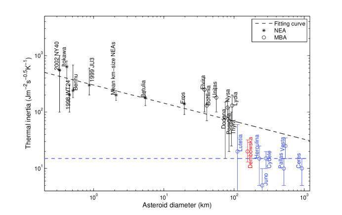
Figure 14: Thermal inertia versus the size of asteroids (Delbo et al., 2007; Delbo & Tanga, 2009).

The rotationally resolved data adopted in present work, uncovers a weak heterogeneous feature between different local longitudes and latitudes of Dembowska. However due to the absence of sufficiently precise observation data, the heterogeneous signal appears to be rather weak to further infer how the surface characteristics differ on various region. Abell & Gaffey (2000) showed that Dembowska may be a heterogeneous body and suggested that this asteroid may bear a large young impact crater. Nevertheless, such impact, if happened, was on a relatively small-scale and would not alter the averaged thermal properties of the global surface. Therefore, we may infer that the entire surface of Dembowska should be covered by a dusty regolith layer with few rocks or boulders on the surface.

On the other hand, we report that the surface temperatures on high latitudes of Dembowska show large seasonal variations, as a result of the large axial tilt between the rotational axis and orbital axis. This kind of seasonal variation can cause significant temperature difference between the south and north region of Dembowska. Thus we argue that the potential heterogeneous features between Dembowska’s south and north region might be induced by the seasonal effects or by large young impact crater. Further investigations should be done to reveal this issue in future.

References

- Abell & Gaffey (2000) Abell P. A., Gaffey M. J., 2000, LPI, 31, 1291A
- Bottke et al. (2005) Bottke, W.F., et al., 2005, Icarus, 179, 63-94
- Bowell et al. (1989) Bowell, E., Hapke, B., Domingue, D., et al., 1989, Application of photometric models to asteroids. In Asteroids II, pp. 524-556
- Cohen et al. (1999) Cohen, M., Walker, R. G., Carter, B., et al., 1999, Aj, 117, 1864
- (5) Database of Asteroid Models from Inversion Techniques. (http://astro.troja.mff.cuni.cz/projects/asteroids3D/web.php)
- Delbo et al. (2007) Delbo, M., et al., 2007, Icarus, 190, 236-249
- Delbo & Tanga (2009) Delbo, M., &, Tanga, P., 2009, PSS, 57, 259-265
- Fowler & Chillemi (1992) Fowler, J.W., & Chillemi, J.R., 1992, IRAS asteroids data processing. In The IRAS Minor Planet Survey, pp. 17-43
- Gaffey et al. (1993) Gaffey, M.J., Burbine, T.H., and Binzel, R.P., 1993, Meteoritics, 28, 161
- Hanuš et al. (2013) Hanuš, J., Marchis, F., Ďurech, J., 2013, Icarus, 226, 1045-1057
- Harris (1998) Harris, A.W., 1998. A Thermal Model for Near-Earth Asteroids, Icarus, 131, 291-301
- (12) JPL Small-Body Database Browser. (http://ssd.jpl.nasa.gov/sbdb.cgi)
- Kaasalainen & Torppa (2001) Kaasalainen, M., & Torppa J., 2001, Icarus, 153, 24
- Kataza et al. (2000) Kataza, H., Okamoto, Y., Takubo, S., et al., 2000, Procspie, 4008, 1144
- (15) Minor Planet Center. (http://www.minorplanetcenter.net/)
- Press et al. (2007) Press W.H., et al., Numerical Recipes, 3th Edition, 2007, Cambridge University Press, NewYork, p. 815
- Rozitis & Green (2011) Rozitis, B., & Green, S.F., 2011, MNRAS, 415, 2042
- Schorghofer (2008) Schorghofer, N., 2008, ApJ, 682, 697-705
- Tedesco (1989) Tedesco, E.F., 1989. Asteroid Magnitude, UBV Colors, and IRAS Albedo and Diameters, in Asteroid II, Univ. Arizona Press, Tucson, pp. 1090-1138
- Torppa et al. (2003) Torppa, J., Kaasalainen, M., Michalowski, T., et al., 2003, Icarus, 164, 346.
- Wright et al. (2010) Wright, E.L., et al., 2010, ApJ, 140, 1868
- Yu, Ji & Wang (2014) Yu, L.L., Ji, J.H., & Wang, S., 2014, MNRAS, 439, 3357-3370
- Yu & Ji (2015) Yu, L.L., & Ji, J.H., 2015, MNRAS, 452, 368-375
- Yu, Ji & Ip (2017) Yu, L.L., Ji, J.H., & Ip, W.H., 2017, Research in Astronomy and Astrophysics, 17, 70