Nonadiabatic Josephson current pumping by microwave irradiation

Abstract

Irradiating a Josephson junction with microwaves can operate not only on the amplitude but also on the phase of the Josephson current. This requires breaking time inversion symmetry, which is achieved by introducing a phase lapse between the microwave components acting on the two† sides of the junction. General symmetry arguments and the solution of a specific single level quantum dot model show that this induces chirality in the Cooper pair dynamics, due to the topology of the Andreev bound state wavefunction. Another essential condition is to break electron-hole symmetry within the junction. A shift of the current-phase relation is obtained, which is controllable in sign and amplitude with the microwave phase and an electrostatic gate, thus producing a “chiral” Josephson transistor. The dot model is solved in the infinite gap limit by Floquet theory and in the general case with Keldysh nonequilibrium Green’s functions. The chiral current is nonadiabatic: it is extremal and changes sign close to resonant chiral transitions between the Andreev bound states.

I Introduction

Microwave irradiation has always been a privileged tool to analyze Josephson junctionsBarone . Photon-assisted Cooper pair transport has been observed in biased junctions Dayem ; Tien-Gordon . Shapiro steps reveal synchronization of the Josephson ac oscillations to the microwave excitationShapiro . In transparent junctions such as quantum point contacts and in junctions made of a quantum dot with a few levels, the Josephson properties are governed by a discrete set of Andreev bound states (ABSs)ABS . In absence of constant bias, nonadiabatic behavior is present even at low irradiation when the microwave frequency (or its harmonics) matches the ABS spacingBergeret1 ; Bergeret2 , causing a sharp decrease of the current amplitude. Resonant microwave can be used as a spectroscopic probe of the ABS dispersion with the phase difference applied on the junctionBretheau .

Josephson currents can be induced either by a magnetic flux of by driving a DC current through a junction. Here we propose a third way of inducing a Josephson current. The main result of this work is that microwave radiation can pump a Josephson current in absence of applied superconducting phase difference and at zero average bias voltage. The required breaking of time inversion symmetry originates from the phase of the microwave radiation, applied as an oscillating voltage $v_{j}(t)$ on each side $j=1,\,2$ of the junction. A nontrivial phase difference $\chi=\chi_{1}-\chi_{2}$ is included in microwave voltage amplitudes $v_{j}(t)=-v_{j}\sin(\Omega t+\chi_{j})$, which introduces chirality in the system. This can be achieved for instance by using a common microwave line bifurcating into two branches, one containing a delay line. A nonzero current appears for $\chi\neq 0,\,\pi$, made of Cooper pairs pumped through the junction. Another and less obvious condition is to break charge conjugation symmetry, e.g. electron-hole symmetry in the junction. As shown below, this can be related to general symmetry considerations. An especially interesting situation is met if the junction is made with a gated quantum dot. The resulting description, adopted in this paper, considers a single noninteracting level, leading to a pair of Andreev bound states (ABS). A simplified “toy-model” description is obtained in the infinite-gap model (IGM), yielding a periodically driven two-level system that can be solved with Floquet formalism. This model captures the essential physics. The general case, involving coupling to the quasiparticle continuum states, is analyzed using nonequilibrium Keldysh Green’s functions.

This effect pertains to the wide class of quantum pumping phenomenaThouless ; Niu . Yet, it is remarkable that it disappears in the adiabatic limit, e.g. when the quantum state of the junction is adiabatically modulated by the microwave radiation. Comparing the microwave frequency to the energy splitting between the phase-dependent ABS, three regimes are obtained : i) a low-frequency regime, which can be described within the IGM by Thouless’ argumentThouless , to lowest order in nonadiabaticity; ii) a high-frequency regime, easily solvable analytically within the IGM; iii) a resonant regime, which generalizes the current anomalies found by Bergeret et al.Bergeret1 ; Bergeret2 , and amenable to a rotating-wave-approximation (RWA) solution in the IGM. Special attention is paid to the cases of superconducting phase differences $\varphi=0,\pi$ where the Josephson current is exclusively due to quantum pumping. For simplicity, this current will be hereafter called “chiral current”, not to be confused with the oriented Josephson current created by a magnetic flux piercing a ring.

One must emphasize that the present pumping mechanism differs from other ones studied in Josephson junctions, such as involving Coulomb blockadePothier , biased junctionsKopnin , or a biased SQUID pumping a normal currentGiazotto ; Russo . Our results also offer a new way to create a highly tunable $\varphi_{0}$-junction with shifted current-phase relation (CPR)Bulaevskii ; Krive ; Egger ; Reynoso ; Buzdin ; Liu ; Sickinger ; Yokohama ; Szombati .

The plan of this work is as follows. After the Introduction (Section 1), Section 2 presents the model and a general analysis of the underlying symmetries. Section 3 contains the Floquet solution of the infinite-gap model : low and high frequency, and close to a resonance (RWA). Section 4 provides the Keldysh solution of the full model and compares it to that of the IGM. Section 5 demonstrates a mapping of the IGM onto a tight-binding lattice chain model, emphasizing the relation between the problem considered in this work and some driven lattice models. Section 6 concludes the paper.

II The model and its symmetries

The time-dependent phases deriving from the applied microwave voltages $v_{1}(t)=-v_{1}\sin(\Omega t+\frac{\chi}{2})$, $v_{1}(t)=-v_{2}\sin(\Omega t-\frac{\chi}{2})$ are defined as:

$$\varphi_{1}=\frac{\varphi}{2}+b_{1}\cos(\Omega t+\frac{\chi}{2}),\;\varphi_{2}=-\frac{\varphi}{2}+b_{2}\cos(\Omega t-\frac{\chi}{2})$$ (1)

with $b_{j}=\frac{2ev_{j}}{\hbar\Omega}>0$. To take a simple example, let us first consider a tunnel junction and work in the adiabatic approximation, e.g. plugging the phase dependences into the equilibrium current-phase relation $I(\varphi_{1},\varphi_{2})=I_{c}\sin(\varphi_{1}-\varphi_{2})$. Using Bessel function expansion, one finds that the microwave radiation only modifies the amplitude of the critical current according to :

$$\langle I\rangle_{dc}=I_{0}[J_{0}(b_{1})J_{0}(b_{2})+2\sum_{n>0}J_{n}(b_{1})J_{n}(b_{2})\cos(n\chi)]\,\sin\varphi.$$ (2)

We show below that going beyond the adiabatic regime in a quantum dot junction makes the microwave affect not only the amplitude but also the phase of the Josephson current.

A specific model of gate-tunable quantum dot Josephson junction is considered now, which bears a single relevant level in front of the energy gap of the superconductors $j=1,2$. Neglecting Coulomb interactions, the Hamiltonian is the following:

$$H = \sum_{kj\sigma}\xi_{kj}c^{\dagger}_{kj\sigma}c_{kj\sigma}\,+\,\Delta\sum_{kj}(c^{\dagger}_{kj\uparrow}c^{\dagger}_{-kj\downarrow}+H.c.)$$

$$+ \varepsilon_{0}\sum_{\sigma}d^{\dagger}_{\sigma}d_{\sigma}\,+\,\sum_{kj,\sigma}t_{j}\big{[}c^{\dagger}_{kj\sigma}d_{\sigma}\,e^{i\varphi_{j}(t)/2}+H.c.\big{]}\;,$$

with $\xi_{k\sigma}=\varepsilon_{k\sigma}-\mu$. The potentials $ev_{j}(t)$ and the phases in the pairing terms have been gauged away to appear in the tunneling terms towards or from the dot.

Unlike the case $v_{j}=0$, the physical properties do not depend in general solely on the phase difference $\varphi(t)=\varphi_{1}(t)-\varphi_{2}(t)$, as seen by performing the gauge transformation $U=\exp\big(-i\nu\varphi_{2}(t)\big{missing})$ (defining $\nu=\frac{1}{2}\sum_{\sigma}d^{\dagger}_{\sigma}d_{\sigma}$). In the presence of time-dependent phases, this transformation correctly eliminates the phase $\varphi_{2}(t)$ but it also yields a time-dependent gate voltage on the dot. Actually, the Hamiltonian (II) does depend on two independent time-dependent fields, e.g. it can lead to quantum pumping if the phase lapse $\chi$ is different from $0$ or $\pi$.

We now investigate the symmetries of the full Hamiltonian (II), first in absence of microwave radiation. Eq. (II) is then parameterized by the phase $\varphi$ and the dot energy $\varepsilon_{0}$. Time inversion $\mathcal{T}$ and charge conjugation $\mathcal{C}$ act on the fermion operators as $\mathcal{T}c_{k\sigma}\mathcal{T}^{-1}=-\sigma c_{-k,-\sigma}$ ($\sigma=\pm$) and $\mathcal{C}c_{k\sigma}\mathcal{C}^{-1}=c^{\dagger}_{k\sigma}$. Using antilinearity of $\mathcal{T}$ leads to $\mathcal{T}H(\varphi,\varepsilon_{0})\mathcal{T}^{-1}=H(-\varphi,\varepsilon_{0})$. The current operator $\hat{J}(\varphi)=\frac{2e}{\hbar}\frac{\partial H}{\partial\varphi}$ transforms according to $-\hat{J}(-\varphi)$, yielding the usual symmetry:

$$\langle\hat{J}(-\varphi,\varepsilon_{0})\rangle=-\langle\hat{J}(\varphi,\varepsilon_{0})\rangle.$$ (4)

On the other hand, charge conjugation applied to Eq. (II) turns $\xi_{ki\sigma},\,t_{i},\,\varepsilon_{0}$ and $\varphi_{i}$ into $-\xi_{ki\sigma},\,-t_{i},\,-\varepsilon_{0}$ and $-\varphi_{i}$. Owing to symmetries of the current with $\xi$ and $t_{i}$, applying $\mathcal{CT}$ leads to:

$$\langle\hat{J}(\varphi,-\varepsilon_{0})\rangle=\langle\hat{J}(\varphi,\varepsilon_{0})\rangle,$$ (5)

a well-known symmetry of the so-called Josephson transistorJTransistor .

Let us now show that this last symmetry is broken by the chiral phase $\chi$. The symmetry operators $\mathcal{T}$ and $\mathcal{C}$ are applied to the time-dependent Hamiltonian $H(\varphi_{j}(t))$. Then $\mathcal{T}H(\varphi_{j}(t),\varepsilon_{0})\mathcal{T}^{-1}=H(-\varphi_{j}(-t),\varepsilon_{0})$ and $-\varphi_{j}(-t)=-\varphi_{j}+b_{j}\cos(\Omega t^{\prime}-\chi_{j})$ with $\varphi_{j}=\pm\frac{\varphi}{2},\chi_{j}=\pm\frac{\chi}{2}$, $t^{\prime}=t+\frac{\pi}{\Omega}$. The latter time translation leaves the time-averaged quantities unchanged, therefore, following the same reasoning as above, one obtains for the DC component of the current:

$$\langle\hat{J}(-\varphi,-\chi,\varepsilon_{0})\rangle_{dc}=-\langle\hat{J}(\varphi,\chi,\varepsilon_{0})\rangle_{dc}.$$ (6)

Similarly, applying $\mathcal{C}$ leaves $\chi$ unchanged, leading to

$$\langle\hat{J}(-\varphi,\chi,-\varepsilon_{0})\rangle_{dc}=-\langle\hat{J}(\varphi,\chi,\varepsilon_{0})\rangle_{dc}.$$ (7)

Eq. (6) shows that time inversion operates both on $\chi$ and $\varphi$, allowing in principle to generate a nonzero “chiral” current with $\varphi=0,\,\pi$ but $\chi\neq 0,\,\pi$. Let us define these currents by $J_{chir,0/\pi}(\chi,\varepsilon_{0})=\langle\hat{J}(0/\pi,\chi,\varepsilon_{0})\rangle_{dc}$. Equations (6,7) lead to:

$$J_{chir,0/\pi}(-\chi,\varepsilon_{0}) = -J_{chir,0/\pi}(\chi,\varepsilon_{0})$$ (8)

$$J_{chir,0/\pi}(\chi,-\varepsilon_{0}) = -J_{chir,0/\pi}(\chi,\varepsilon_{0})$$ (9)

Therefore the chiral current not only changes sign with $\chi$ - Equation (8) is similar to Equation (4) - but Equation (9) show that it also changes sign with $\varepsilon_{0}$, contrarily to the current generated by $\varphi$ only (Equation (5)). This nontrivial connection between time inversion and electron-hole symmetries is a fingerprint of this chiral Josephson current. Notice that a normal current pumped through a gated quantum dot is also found to change sign with the gate voltageKouwenhoven .

III The infinite-gap limit: Floquet analysis

III.1 The Hamiltonian

Let us first consider the infinite-gap model (IGM) limit Jonckheere . The subspaces of even and odd number states on the dot become decoupled and only the even states may mediate a Josephson coupling. Within the even number space, a pseudospin mapping of the empty and doubly occupied states is defined as: $\hat{\tau}_{+}=d^{\dagger}_{\uparrow}d^{\dagger}_{\downarrow}$ and $\hat{\tau}_{z}=2d^{\dagger}_{\uparrow}d^{\dagger}_{\downarrow}d_{\downarrow}d_{\uparrow}-1$, yielding a driven two-level system:

$$H_{\infty}(t)=\sum_{j=1,2}\gamma_{j}\Big{[}e^{-i\varphi_{j}(t)}\hat{\tau}_{+}+e^{i\varphi_{j}(t)}\hat{\tau}_{-}\Big{]}+\varepsilon_{0}\hat{\tau}_{z}\;,$$ (10)

where $\gamma_{j}=\pi\nu(0)t_{j}^{2}$ is the pair hopping amplitude [$\nu(0)$ is the metallic density of states].

This model can be solved with Floquet theoryGrifoni . The wavefunction $\Psi(t)$ evolves according to $i\dot{\Psi}(t)=H_{\infty}(t)\Psi(t)$ (taking $\hbar=1$). For the $T$-periodic Hamiltonian $H_{\infty}(t)$ ($T=2\pi/\Omega$), there exists a set of Floquet pseudo-energies ($\epsilon_{\alpha}$) and a periodic basis of wave-functions $(\phi_{\alpha})$ with period $T$. A basis solution $\Psi_{\alpha}(t)$ can be written as $\Psi_{\alpha}(t)=e^{-i\epsilon_{\alpha}t}\phi_{\alpha}(t)$.

Fourier expansion of $H_{\infty}(t)$ and $\phi_{\alpha}(t)$ gives:

$$H_{\infty}(t)=\sum_{n=-\infty}^{+\infty}\tilde{H}_{\infty n}e^{in\Omega t}\quad\textrm{,}\quad\phi_{\alpha}(t)=\sum_{n=-\infty}^{+\infty}\tilde{\phi}_{\alpha n}e^{in\Omega t},$$ (11)

where, defining $\gamma_{i,n}=\gamma_{i}J_{n}(b_{i})(i=1,2)$

$$\tilde{H}_{\infty,0} = \big{(}\gamma_{1,0}e^{-i\frac{\varphi}{2}}+\gamma_{2,0}e^{i\frac{\varphi}{2}}\big{)}\,\tau_{+}$$ (12)

$$+ \big{(}\gamma_{1,0}e^{i\frac{\varphi}{2}}+\gamma_{2,0}e^{-i\frac{\varphi}{2}}\big{)}\,\tau_{-}+\varepsilon_{0}\tau_{z},$$

and for all integers $n\neq 0$:

$$\tilde{H}_{\infty,n} = [(-i)^{n}\big{(}\gamma_{1,n}{e}^{-{i}\frac{\varphi}{2}}{e}^{{i}n\frac{\chi}{2}}+\gamma_{2,n}{e}^{{i}\frac{\varphi}{2}}{e}^{-{i}n\frac{\chi}{2}}]\,\tau_{+}$$ (13)

$$+ [(i^{n}\big{(}\gamma_{1,n}{e}^{i\frac{\varphi}{2}}{e}^{{i}n\frac{\chi}{2}}+\gamma_{2,n}{e}^{-{i}\frac{\varphi}{2}}{e}^{-{i}n\frac{\chi}{2}}]\,\tau_{-}.$$

The Fourier series defined in Eq. (11) leads to

$$\sum_{m=-\infty}^{\infty}\tilde{H}^{FL}_{\infty nm}\phi_{\alpha m}=\epsilon_{\alpha}\phi_{\alpha n},$$ (14)

where

$$\tilde{H}^{FL}_{\infty nm}=\tilde{H}_{\infty,n-m}+n\Omega\delta_{nm}.$$ (15)

Noting $\tilde{\phi}_{\alpha}=\begin{pmatrix}\ldots,\tilde{\phi}_{\alpha-1},\tilde{\phi}_{\alpha 0},\tilde{\phi}_{\alpha 1},\ldots\end{pmatrix},$ Eq. (14) can be cast in matrix form:

$$\tilde{H}^{FL}_{\infty}\tilde{\phi}_{\alpha}=\epsilon_{\alpha}\tilde{\phi}_{\alpha}.$$ (16)

The DC-current $I_{\alpha}$ associated to state $\ket{\Psi_{\alpha}(t)}$ is defined as $I_{\alpha}=2e\overline{\bra{\Psi_{\alpha}(t)}\frac{\partial H_{\infty}(t)}{\partial\varphi}\ket{\Psi_{\alpha}(t)}}$ where $\overline{f(t)}=\frac{1}{T}\int_{0}^{T}f(t){dt}$. Eq. (11) leads to

$$\overline{\bra{\Psi_{\alpha}(t)}\frac{\partial H_{\infty}(t)}{\partial\varphi}\ket{\Psi_{\alpha}(t)}}=\bra{\tilde{\phi}_{\alpha}}\frac{\partial\tilde{H}^{FL}_{\infty}}{\partial\varphi}\ket{\tilde{\phi}_{\alpha}}.$$ (17)

According to Hellman-Feynman theorem, $\bra{\tilde{\phi}_{\alpha}}\frac{\partial\tilde{H}^{FL}}{\partial\varphi}\ket{\tilde{\phi}_{\alpha}}=\frac{\partial\epsilon_{\alpha}}{\partial\varphi}$. Therefore, the DC-current $I_{\alpha}$ in Floquet eigenstate becomes

$$I_{\alpha}(\varphi,\chi,\epsilon_{0})=2e\frac{\partial\epsilon_{\alpha}}{\partial\varphi}(\varphi,\chi,\epsilon_{0}),$$ (18)

generalizing the Josephson equation to a Floquet state. The DC-current $I_{\alpha}$ can be calculated from Eq. (18) once the pseudo-energy $\epsilon_{\alpha}$ are known from Eq. (16).

III.2 Low-frequency limit

In this section, the microwave frequency $\Omega$ is supposed to be small compared to the other relevant energies. The quasiadiabatic approximation can then be used.

Let us call $(\ket{\Psi_{+}(t)},\ket{\Psi_{-}(t)})$, the instantaneous basis of the system, such that $H_{\infty}(t)\ket{\Psi_{\pm}(t)}=E_{\pm}(t)\ket{\Psi_{\pm}(t)}$, where

$$E_{\pm}(t)=\pm\sqrt{\epsilon_{0}^{2}+\gamma_{1}^{2}+\gamma_{2}^{2}+2\gamma_{1}\gamma_{2}\cos(\varphi_{1}(t)-\varphi_{2}(t))}.$$ (19)

with $\varphi_{1,2}(t)$ given by Equation (1). Each wavefunction $\ket{\Psi(t)}$ can be decomposed on this basis : $\ket{\Psi(t)}=c_{+}(t)\ket{\Psi_{+}(t)}+c_{-}(t)\ket{\Psi_{-}(t)}$. Following Thouless Thouless (see also Xiao Xiao )and choosing $\ket{\Psi(0)}=\ket{\Psi_{+}(0)}$, we have

$$\ket{\Psi(t)}=\ket{\Psi_{+}(t)}-i\ket{\Psi_{-}(t)}\frac{\langle\Psi_{-}(t)|\frac{\partial}{\partial t}\Psi_{+}(t)\rangle}{E_{+}(t)-E_{-}(t)}.$$ (20)

The DC-current of the state $\ket{\Psi(t)}$ is $I=2e\overline{\bra{\Psi(t)}\frac{\partial H(t)}{\partial\varphi}\ket{\Psi(t)}}$ and one finds

$$I=2e(\overline{\frac{\partial E_{+}}{\partial\varphi}}-\overline{C^{+}_{\varphi,t}}),$$ (21)

where

$$C^{+}_{\varphi,t}=i\left(\langle{\frac{\partial\Psi_{+}}{\partial\varphi}|\frac{\partial\Psi_{+}}{\partial t}}\rangle-\langle{\frac{\partial\Psi_{+}}{\partial t}|\frac{\partial\Psi_{+}}{\partial\varphi}}\rangle\right)$$ (22)

is the Berry curvature in the $(\Omega t,\varphi)$ variables. The first term in Eq. (21) is the adiabatic contribution and the second one is the first nonadiabatic correction. It is straightforward to check that if $\varphi=0,\pi$ the adiabatic current $2e\frac{\partial E_{+}}{\partial\varphi}=\frac{-\gamma_{1}\gamma_{2}\sin(\varphi_{1}(t)-\varphi_{2}(t))}{|E_{-}(t)|}$ has a zero time average, whatever the relative phase $\chi$ of the microwave fields. Actually, the adiabatic current is a function of $\varphi(t)=\varphi_{1}(t)-\varphi_{2}(t)=\varphi+b_{1}\cos(\Omega t+\frac{\chi}{2})-b_{2}\cos(\Omega t-\frac{\chi}{2})$, which verifies $\varphi(t+\frac{T}{2})=-\varphi(t)$ and thus has a zero integral on the interval $[0,T]$footnote . Therefore the chiral current at $\varphi=0,\,\pi$ is intrinsically nonadiabatic, and

$$I_{chir,0/\pi}=-2e\,\overline{C^{+}_{\varphi,t}}\lvert_{\varphi=0/\pi}.$$ (23)

This justifies the word “chiral” used throughout the paper : chirality is related to the properties of the ABS wavefunctions. The Berry curvature is expressed by rewriting the Hamiltonian as $H_{\infty}(t)=\vec{h}(t).\vec{\sigma}$ with:

$$\left\{\begin{array}[]{ll}\vec{h}(t)=\Big{(}\frac{\Gamma(t)+\Gamma^{*}(t)}{2},i\frac{\Gamma(t)-\Gamma^{*}(t)}{2},\epsilon_{0}\Big{)}^{t}\\ \Gamma(t)=\sum_{j=1,2}\gamma_{j}e^{-i\varphi_{j}(t)}\\ \vec{\sigma}=(\sigma_{x},\sigma_{y},\sigma_{z})\end{array},\right.$$ (27)

where $|\vec{h}(t)|=|E_{\pm}(t)|$. Expressing each of the three terms separately leads to

$$\frac{1}{|\vec{h}|^{3}}\vec{h}.(\partial_{\varphi}\vec{h}\times\partial_{t}\vec{h})=-2C^{+}_{\varphi,t}.$$ (28)

Eqs. (23) and (28) then yieldHasanKane :

$$I_{\varphi=0}=\frac{e\Omega}{h}\frac{1}{|\vec{h}|^{3}}\int_{0}^{2\pi}\vec{h}.(\partial_{\varphi}\vec{h}\times\partial_{(\Omega t)}\vec{h}){d(\Omega t)}$$ (29)

Interestingly, this results in:

$$I_{\varphi=0}=-\frac{e\Omega}{2\pi}\frac{\partial}{\partial\chi}\left(\int_{0}^{2\pi}\frac{\epsilon_{0}}{|E_{\pm}(\Omega t)|}{d(\Omega t)}\right).$$ (30)

This equation shows an intriguing formal similarity between the pumped Josephson current, as a function of the microwave phase $\chi$, and the equilibrium Josephson current, expressed as the derivative of the ABS energy with respect to the superconducting phase. Yet in Eq. (30), the ABS energy is replaced by its inverse.

III.3 High-frequency limit

Perturbation theory can be used in the case of large microwave frequency $\Omega$ and small amplitudes $b_{1}$, $b_{2}$ of the microwaveAoki . The Floquet Hamiltonian is split as a diagonal and nondiagonal part: $H_{\infty}^{FL}=H^{FL}_{diag}+\rho\,h$ where $H^{FL}_{diag}$ is diagonal, and $\rho\,h$ is non diagonal ($\rho<<1$). The resulting effective Hamiltonian takes the form

$$H^{FL}_{\infty,eff}={e}^{-i\rho S}H_{\infty}^{FL}{e}^{i\rho S}.$$ (31)

The matrix $S$ is chosen according to

$$\bra{\alpha}S\ket{\beta}=-\frac{\bra{\alpha}h\ket{\beta}}{\epsilon_{\alpha}-\epsilon_{\beta}},$$ (32)

where $\ket{\alpha}=\ket{\pm,p}$, $\ket{\beta}=\ket{\pm,q}$ (with $p\neq q$ integers) are eigenstates of $H^{FL}_{diag}$ with eigenvalues $\epsilon_{r}=\pm\sqrt{\varepsilon_{0}^{2}+\left|\tilde{z}\right|^{2}}+r\Omega$ and $\tilde{z}=\gamma_{1}e^{-i\varphi/2}+\gamma_{2}e^{i\varphi/2}$ ($r=p,q$).

Expanding the effective Hamiltonian in powers of $b$ leads to $H^{FL}_{\infty,eff}\simeq H^{FL}_{\infty,diag}+\frac{\rho^{2}}{2}[h,S]$. The effective Hamiltonian becomesAoki :

$$H^{FL}_{\infty,eff}=H^{FL}_{\infty,diag}+\frac{1}{\Omega}[\tilde{H}_{\infty,1},\tilde{H}_{\infty,-1}]1_{N\times N}$$ (33)

where $\tilde{H}_{\infty,1}$ (respectively $\tilde{H}_{\infty,-1}$) is the $1$st harmonics (respectively the $-1$th) of the periodic Hamiltonian $H_{\infty(t)}$, which leads to:

$$\frac{1}{\Omega}[\tilde{H}_{\infty 1},\tilde{H}_{\infty-1}]=\frac{1}{\Omega}\gamma_{1}\gamma_{2}b_{1}b_{2}\sin\varphi\sin\chi\,\sigma_{z}.$$ (34)

The effective Hamiltonian $H^{FL}_{\infty,eff}$ is block diagonal and only the zeroth harmonic is considered by periodicity of the energy spectrum. Denoting $H_{\infty,eff}=H^{FL}_{\infty,eff,0}$ leads to

$$H_{\infty,eff}=\big{(}\gamma_{1}e^{-i\frac{\varphi}{2}}+\gamma_{2}e^{i\frac{\varphi}{2}}\big{)}\,\tau_{+}+\big{(}\gamma_{1}e^{i\frac{\varphi}{2}}+\gamma_{2}e^{-i\frac{\varphi}{2}}\big{)}\,\tau_{-}+\tilde{\varepsilon}_{0}\tau_{z},$$ (35)

with the dot level renormalized by the microwave:

$$\tilde{\epsilon}_{0}=\epsilon_{0}+\frac{1}{\Omega}\gamma_{1}\gamma_{2}b_{1}b_{2}\sin\varphi\sin\chi.$$ (36)

The eigenvalues $H_{\infty,eff}$ are:

$$\tilde{E}_{0,\pm}=\pm\sqrt{\tilde{\epsilon}_{0}^{2}(\varphi)+\gamma_{1}^{2}+\gamma_{2}^{2}+2\gamma_{1}\gamma_{2}\cos\varphi}.$$ (37)

Using the fact that $I=2e\partialderivative{\tilde{E}_{0,\pm}}{\varphi}$, the chiral current at $\varphi=0$ $(\zeta=1)$ or $\varphi=\pi$ $(\zeta=-1)$ is given by:

$$I_{chir,0/\pi}=2e\frac{\epsilon_{0}\gamma_{1}\gamma_{2}b_{1}b_{2}\sin\chi}{\Omega\sqrt{\epsilon_{0}^{2}+(\gamma_{1}+\zeta\gamma_{2})^{2}}}.$$ (38)

Eq. (38) provides evidence for a Josephson current induced solely by the chiral phase $\chi$. This current is quadratic in the microwave amplitude and it changes sign with the dot level energy $\varepsilon_{0}$, in agreement with the general symmetry relations discussed above. If $\varphi=\pi$ and for a symmetric junction, it shows a jump at $\varepsilon_{0}=0$.

III.4 Solution close to resonance

We use the same method as Bergeret et al. Bergeret2 to find the analytical current close to resonance e.g. when the microwave frequency matches the ABS spacing. Let us consider the infinite-gap Hamiltonian:

$$H_{\infty}(t)=\begin{pmatrix}\epsilon_{0}&\Gamma(t)\\ \Gamma^{*}(t)&-\epsilon_{0}\end{pmatrix},$$ (39)

with $\Gamma(t)=\sum_{j=1,2}\gamma_{j}e^{-i\varphi_{j}(t)}=|\Gamma(t)|e^{i\beta(t)}$. The instantaneous eigenvalues of Eq. (39) take the form $E_{\pm}(t)=\pm E_{A}(t)=\pm\sqrt{\epsilon_{0}^{2}+|\Gamma(t)|^{2}}$, and the orthonormal eigenvectors are the following:

$$\ket{\Psi_{+}}=\begin{pmatrix}\cos\frac{\theta}{2}e^{i\beta}\\ \sin\frac{\theta}{2}\end{pmatrix}\quad\ket{\Psi_{-}}=\begin{pmatrix}-\sin\frac{\theta}{2}e^{i\beta}e^{i\alpha}\\ \cos\frac{\theta}{2}e^{i\alpha}\end{pmatrix},$$ (40)

where $\cos[\theta(t)]=\frac{\epsilon_{0}}{E_{A}(t)}$, $\sin[\theta(t)]=\frac{|\Gamma(t)|}{E_{A}(t)}$, $\alpha$ is an arbitrary phase and $H_{\infty}(t)\ket{\Psi_{\pm}}=\pm E_{A}(t)\ket{\Psi_{\pm}}$.

Let us now rotate to the instantaneous basis $\Big{(}\ket{\Psi_{+}},\ket{\Psi_{-}}\Big{)}$. In this new basis, $\ket{\tilde{\Psi}}$ is related to $\ket{{\Psi}}$ in the old basis by $\ket{\tilde{\Psi}}=U\ket{\Psi}$ where U is a unitary matrix, obtained from Eq. (40):

$$U^{\dagger}=\begin{pmatrix}\cos\frac{\theta}{2}e^{i\beta}&-\sin\frac{\theta}{2}e^{i\beta}e^{i\alpha}\\ \sin\frac{\theta}{2}&\cos\frac{\theta}{2}e^{i\alpha}\end{pmatrix}.$$ (41)

The gauge $\alpha(t)$ eliminates the $\hat{\tau}_{x}$ term in the Hamiltonian $\hat{H}_{A}$. It must satisfy

$$\dot{\beta}\sin\theta\cos\alpha+\dot{\theta}\sin\alpha=0.$$ (42)

The new Hamiltonian associated to $\ket{\tilde{\Psi}}$ is $\hat{H}_{A}=UHU^{\dagger}+i\derivative{U}{t}U^{\dagger}$. It is given by:

$$\hat{H}_{A}(t)=[E_{A}(t)+\dot{\beta}\cos^{2}\frac{\theta}{2}-\frac{\dot{\beta}+\dot{\alpha}}{2}]\hat{\tau}_{z}-\frac{\dot{\theta}}{2\cos\alpha}\hat{\tau}_{y}+\frac{\dot{\beta}+\dot{\alpha}}{2}.$$ (43)

The current operator is defined as $I_{\infty}=2e\partialderivative{H_{\infty}}{\varphi}$. From now on, we choose a symmetric junction ($\gamma_{1}=\gamma_{2}=\gamma_{0}$) and symmetrical microwave amplitudes ($b_{1}=b_{2}=b$). The angle $\beta$ does not depend anymore on $\varphi$. Using Eq. (39), the current operator takes the form $I_{\infty}=2e\,\partialderivative{|\Gamma(t)|}{\varphi}[\cos\beta\,\hat{\tau}_{x}-\sin\beta\,\hat{\tau}_{y}]$. In the new basis, the current operator becomes $\hat{I}_{A}=UI_{\infty}U^{\dagger}$, thus:

$$\hat{I}_{A}=2e\partialderivative{|\Gamma(t)|}{\varphi}[\cos\theta\,\hat{\tau}_{z}+\cos\theta\cos\alpha\,\hat{\tau}_{x}-\cos\theta\sin\alpha\,\hat{\tau}_{y}].$$ (44)

According to Ref. Bergeret2, , the DC-current is calculated by i) modifying the Hamiltonian by adding to it a term proportional to $\hat{I}_{A}$ and defining a generating function for the time-averaged current; ii) going to Floquet space and calculating the long-time Floquet evolution operator at times $nT(n>>1)$. This defines a generalized Josephson energy and the averaged current is obtained by a double derivative:

$$I_{DC}=\partialderivative{E(\eta,\mu)}{\mu}\Big{|}_{\eta,\mu=0}\partialderivative{E(\eta,\mu)}{\eta}\Big{|}_{\eta,\mu=0},$$ (45)

with $\pm E(\eta,\mu)$ the eigenvalues of the matrix $\hat{M}=\frac{1}{T}\int_{0}^{T}\hat{H}_{n}(t)dt+\mu\hat{\tau}_{z}$. This is the the first term in the expansion of the effective evolution operator in the detuning from the n-th order resonance, expressed by the small parameter $(E_{A}-n\frac{\Omega}{2})/\Omega$. The Hamiltonian $\hat{H}_{n}(t)$ is such that:

$$\hat{H}_{n}(t)=e^{in\Omega t\hat{\tau}_{z}/2}[\hat{H}_{A}(t)+\eta\hat{I}_{A}-n\frac{\Omega}{2}\hat{\tau}_{z}]e^{-in\Omega t\hat{\tau}_{z}/2}.$$ (46)

After some simplifications, one obtains:

$$\frac{1}{T}\int_{0}^{T}dt\hat{H}_{n}(t)=\frac{1}{T}\int_{0}^{T}dt\left[\hat{\tau}_{z}\left(E_{A}-n\frac{\Omega}{2}\right)-\hat{\tau}_{x}\left(\frac{\dot{\theta}}{2\cos\alpha}+\eta\cos\theta\sin\alpha\partialderivative{|\Gamma|}{\varphi}\right)\sin(n\Omega t)\right].$$ (47)

Let us first consider $\varphi=0$, with $b$ small. After several manipulations (see Appendix A), Eq. (47) yields the effective RWA Hamiltonian close to the first-order resonance:

$$\frac{1}{T}\int_{0}^{T}\hat{H}_{1}(t)dt = \hat{\tau}_{z}\left(\bar{E}_{0}-\frac{\Omega}{2}\right)$$

$$+ \hat{\tau}_{x}\frac{\gamma_{0}b}{2E_{0}}\Big{[}\Omega\cos\frac{\chi}{2}F_{1}-\eta\epsilon_{0}\sin\frac{\chi}{2}F_{2}\Big{]},$$

where $E_{0}=\sqrt{\epsilon_{0}^{2}+4\gamma_{0}^{2}}$ is the Andreev energy without microwaves, $\bar{E}_{0}=E_{0}(1-\frac{\gamma_{0}^{2}}{E_{0}^{2}}b^{2}\sin^{2}\frac{\chi}{2})$ and $F_{1},F_{2}$ are constants defined in Appendix A. The eigenvalues of $\hat{M_{1}}$ verify:

$$E^{2}(\eta,\mu) = \left(\bar{E}_{0}-\frac{\Omega}{2}+\mu\right)^{2}$$ (49)

$$+ \frac{\gamma_{0}^{2}b^{2}}{4E_{0}^{2}}\Big{[}\Omega\cos\frac{\chi}{2}F_{1}-\eta\epsilon_{0}\sin\frac{\chi}{2}F_{2}\Big{]}^{2}.$$

Finally, the chiral current close to the first resonance is:

$$I_{chir,0}(\chi,\varepsilon_{0})=\frac{e\gamma_{0}^{2}b^{2}\varepsilon_{0}}{E_{0}}\frac{(\Omega-2\bar{E}_{0})F_{1}F_{2}\sin\chi}{(\Omega-2\bar{E}_{0})^{2}+4\gamma_{0}^{2}b^{2}F_{1}^{2}\cos^{2}\frac{\chi}{2}}.$$ (50)

This resonance is plotted in Figure 6, together with the full Keldysh result (see next Section). The resonance width is given by $2\gamma_{0}bF_{1}|\cos\frac{\chi}{2}|$ and the maximal chiral current is anharmonic in $\chi$:

$$I_{chir,0}^{max}\sim\frac{e\gamma_{0}bF_{2}|\varepsilon_{0}\sin\frac{\chi}{2}|}{2\hbar E_{0}}$$ (51)

Let us consider now the case $\varphi=\pi$. The first harmonics $(\Omega=2E_{A})$ was calculated above to first order in the resonance detuning. Eq. (47) is used and $E_{0}=\left|\epsilon_{0}\right|$ stands for the Andreev state energy without microwaves. Defining $\bar{E}^{\prime}_{0}=E_{0}(1+\frac{\gamma_{0}^{2}}{E_{0}^{2}}b^{2}\sin^{2}\frac{\chi}{2})$ leads to

$$E^{2}(\eta,\mu) = \left(\bar{E}^{\prime}_{0}-\frac{\Omega}{2}+\mu\right)^{2}$$

$$+ \frac{\gamma_{0}^{2}b^{2}}{\pi^{2}E_{0}}\left[\Omega\sin\frac{\chi}{2}G_{1}+\frac{2}{3}\eta\epsilon_{0}\cos\frac{\chi}{2}G_{2}\right]^{2}$$

and

$$I_{chir,\pi}(\chi,\epsilon_{0})=-\frac{8e\gamma_{0}^{2}b^{2}\epsilon_{0}}{3\pi^{2}E_{0}}\frac{(\Omega-2\bar{E}^{\prime}_{0})G_{1}G_{2}\sin\chi}{(\Omega-2\bar{E}^{\prime}_{0})^{2}+\frac{16}{\pi^{2}}\gamma_{0}^{2}b^{2}G_{1}^{2}\sin^{2}\frac{\chi}{2}},$$

where $G_{1},G_{2}$ are defined in Appendix A.

Comparing to $\varphi=0$, notice the sign change and the different $\chi$-dependence of the resonance width $\sim\frac{4}{\pi}\gamma_{0}bG_{1}|\sin\frac{\chi}{2}|$ and of the maximal chiral current $I_{chir,\pi}^{max}\sim\frac{2e\gamma_{0}bG_{2}}{3\pi\hbar}|\cos\frac{\chi}{2}|$.

Interestingly, the dependence in $\chi$ of $I_{max}$, Equation (51), recalls that of an equilibrium junction made of a resonant dot, varying as $|\sin\frac{\varphi}{2}|$ due to closure of the Andreev gap at $\varphi=\pi$. In the present case, the ABS are gapped but at resonance the driven system behaves as gapless, generating the anharmonicity in $\chi$.

III.5 Numerical solution

As an example of a nonperturbative result, Fig. 1a shows the Floquet current for different microwave amplitudes and Fig. 1b shows the Floquet spectrum for $\chi=\frac{\pi}{2}$ and large $b_{1}=b_{2}$. We note $I_{1}=\frac{e}{\hbar}\gamma_{1}$. The anticrossings are shifted in phase and clearly asymmetric, which reflects time symmetry breaking and the chirality. To calculate the time-averaged Josephson current, one needs in principle to fix initial conditions e.g. perform an average over an initial distribution of Floquet eigenstates. Here we use a simple protocol, which perfectly maps onto the ground state Andreev current for zero microwave amplitude $b_{1,2}=0$. As $\varphi$ increases, the zero-th order Floquet state $\Psi_{n=0,-}$ is followed everywhere except in the centre of the anticrossing where it jumps across the anticrossing gap. As in Refs. Bergeret1 ; Bergeret2 , one obtains dips in the current when the ABS splitting is a multiple of the microwave frequency. Again, there is a strong asymmetry in the current, due to the chiral phase $\chi$. Most importantly, nonzero “chiral” currents are obtained $\varphi=0,\pi$.

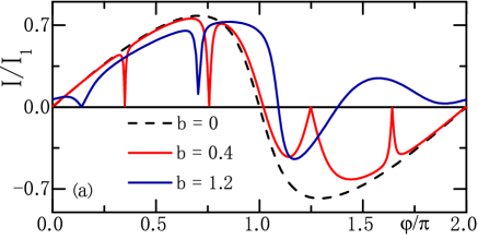
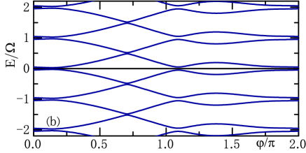
Figure 1: (Color online). (a) Current-phase relation in the chiral case ($\chi=\frac{\pi}{2}$), with $\varepsilon_{0}=0.5$, $\Omega=1.75$, $\gamma_{1}=\gamma_{2}=1$, $b_{1}=b_{2}=b=0,0.4,1.2$, showing the nonadiabatic resonances and the chiral asymmetry around $\varphi=\pi$. (b) Floquet spectrum in the energy-phase plane, with $b_{1}=b_{2}=b=1.2$. The dotted lines indicate the equilibrium ABS.

IV General solution: Keldysh analysis

The microwave perturbs the ABS, also causing transitions towards the quasiparticle continuum, an effect negelcted in the infinite gap approximation. Let us fully solve the model Hamiltonian (II) by using Keldysh nonequilibrium Green’s functions. Those allow to obtain the spectral density and the dc current from Hamiltonian (II)Nozieres ; Cuevas ; Regis1 . The Keldysh Green’s function (GF) $\hat{G}^{+,-}$ is defined in the Nambu space spanned by the Pauli matrix $\hat{\tau}$ by:

$$\hat{G}_{ab}^{+-}(\tau,\tau^{\prime})=i\begin{pmatrix}\langle c^{\dagger}_{b\uparrow}(\tau^{\prime})c_{a\uparrow}(\tau)&\langle c^{\dagger}_{b\uparrow}(\tau^{\prime})c^{\dagger}_{a\downarrow}(\tau)\\ \langle c_{b\downarrow}(\tau^{\prime})c_{a\uparrow}(\tau)\rangle&\langle c_{b\downarrow}(\tau^{\prime})c^{\dagger}_{a\downarrow}(\tau)\end{pmatrix},$$ (54)

and $\hat{G}_{ab}^{A}(\tau,\tau^{\prime})$ obtained by replacing all correlators $\langle A(\tau^{\prime})B(\tau)\rangle$ by $\theta(\tau-\tau^{\prime})\langle\{A(\tau^{\prime}),B(\tau)\}\rangle$ ($a,b=1,2,d$). Due to time periodicity, double Fourier transform is performed as:

$$\hat{G}_{ab,nm}(\omega)=\int\int d\tau d\tau^{\prime}e^{i\omega(\tau-\tau^{\prime})}e^{i\Omega(n\tau-m\tau^{\prime})}\hat{G}_{ab}(\tau,\tau^{\prime})$$ (55)

The Dyson equation implies a product in frequency space and a convolution product in the indices $n$:

$$\hat{G}^{R,A} = \hat{g}^{R,A}+\hat{g}^{R,A}\hat{\Sigma}^{R,A}\hat{G}^{R,A}$$

$$\hat{G}^{+-} = (\hat{I}+\hat{G}^{R}\hat{\Sigma}^{R})\hat{g}^{+-}(\hat{I}+\hat{\Sigma}^{A}\hat{G}^{A})$$ (56)

where $\Sigma_{jd}^{R,A}$ and the bare Green’s functions are defined in Appendix B.

The dc current is calculated between lead $1$ and the dot (the trace is in Nambu space):

$$I=\frac{e}{\hbar}\tr\{\sigma_{z}\int d\omega\sum_{n}\tilde{\Sigma}_{d1,n}\hat{G}^{+-}_{1d,0n}(\omega)$$

$$-\tilde{\Sigma}_{1d,n}\hat{G}^{+-}_{d1,0n}(\omega)\Big{\}}$$ (57)

where $\tilde{\Sigma}_{jd,n}$ is the $n$th harmonic of the periodic self-energy $\Sigma_{jd}=\Sigma_{jd}^{R,A}$. Details are given in Appendix B.

Solving for the Dyson equation and taking the $n=m=0$ component yields the DC Josephson current $I(\varphi,\chi,\varepsilon_{0})$, which is a function of i) the superconducting phase difference $\varphi$, ii) the chiral (microwave) phase difference $\chi$, iii) the microwave amplitudes $b_{1,2}$ and frequency $\Omega$ (one takes $\hbar=1$ in all the figures), and iv) the dot parameters $\varepsilon_{0}$ and $t_{1,2}$. The current is in units of $I_{0}=\frac{e}{\hbar}\Delta$. The values $\eta_{s}=10^{-3}\Delta,\eta_{d}=10^{-5}\Delta$ are used for the inelastic parameters and temperature is $T=0$, unless specified otherwise.

Fig. 2a shows the current-phase relation in the chiral case, for moderate $b_{1}=b_{2}=0.4$. The evidence for chirality is confirmed by plotting the effective density of states, defined as $\rho_{d}=2\imaginary(G^{a}_{dd}-G^{r}_{dd})$, where the anticrossings causing the resonances are asymmetric. This qualitatively confirms the trends obtained in the IGM (Section III, Fig. 1). Notice the logarithmic scale in the amplitude. Some broadening is due to the inelastic parameters but it is mainly due to coupling to the continuum via the microwave excitation. This spectrum could be observed by microwaveBretheau or tunnelPillet ABS spectroscopy. The phase shift and the chiral currents (at $\varphi=0,\pi$) are very small for those excitation amplitudes. Fig. 3 instead shows the case of a higher microwave amplitude. The phase shift and nonzero chiral currents are quite visible. Again, these features are similar to those found in the infinite-gap model (Fig. 1). Since the microwave radiation couples strongly the equilibrium ABS to the continuum, only a qualitative agreement can be found.

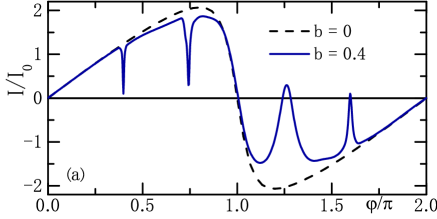
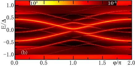
Figure 2: (Color online). (a) Current-phase relation in the chiral case ($\chi=\frac{\pi}{2}$), with $\varepsilon_{0}=0.1\Delta$, $\Omega=0.35\Delta$, $t_{1}=t_{2}=0.6\Delta$, $b_{1}=b_{2}=b=0.4$, showing the nonadiabatic resonances and the chiral asymmetry around $\varphi=\pi$. (b) Density of states (see text) in the energy-phase plane, with the same parameters.

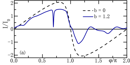
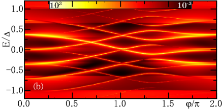
Figure 3: (Color online). Idem as Fig. (2), same parameters except $b_{1}=b_{2}=1.2$. The chiral currents at $\varphi=0,\pi$ are apparent despite the nonresonant behaviour.

Let us now set $\varphi=0$ or $\pi$ and analyze the chiral current $I_{chir}$. It is amplified when a resonance occurs at $\varphi=0$ or $\pi$. We focus here on small microwave amplitudes which lead to small chiral currents but display more clearly the main quantitative features. This situation can be compared to an equilibrium tunnel junction where the curent is harmonic except for a resonant dot. Fig. 4 indeed shows $I_{chir,0}(\Omega)$ and $I_{chir,\pi}(\Omega)$ as a function of $\Omega$. The chiral current changes sign at resonance. For $\varphi=0$, the main resonance indeed occurs at $\Omega\sim 2E_{A}(\varphi=0)$, e.g. matching the ABS spacing. A thin and asymmetric resonance also appears around $\Omega=1.4\Delta$, due to a transition from the lowest ABS to the upper gap edge. Contrarily to the main resonance between ABS, it depends strongly on the gap smearing parameter $\eta_{s}$ as shown in Fig. 5a. The subtle dependence of a resonant property with the coupling to quasiparticle states and with the $\eta$’s has been discussed in Ref. Regis2, for a related problem. In the case $\varphi=\pi$, the first harmonic resonance around $\Omega=0.3\Delta$ is quite soft and, remarkably, an intense and narrow second harmonic ($\Omega\sim E_{A}(\varphi=\pi)\simeq 0.15\Delta$) resonance appears.

In the above-described pumping mechanism, the phase $\chi$ replaces $\varphi$ as the driving phase for the Josephson current. Far from resonance, $I_{chir}$ is approximately sinusoidal with $\chi$. Close to resonance, strong nonharmonicity and a change of sign are instead obtained (Fig. 5b). Fig. 5c shows the chiral current as a function of the dot level $\varepsilon_{0}$ at fixed $\varphi=\pi$ and $\chi=\frac{\pi}{2}$, displaying the symmetry expressed by Eq. (7). More generally, the symmetries (6) and (7) were numerically checked for $\varphi\neq 0$. Remarkably, the rapid change close to $\varepsilon_{0}=0$ is in agreement with the analytical formula (Equation (38)) obtained within the IGM. Moreover, asymmetric $\gamma$’s, or a nonzero temperature, makes $I_{chir}$ linear with $\varepsilon_{0}$ (Fig. 5c). This behaviour reminds that of a resonant symmetric equilibrium junction where at zero temperature the current experiences a jump at phase $\varphi=\pi$.

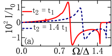
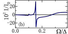
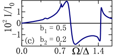
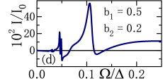
Figure 4: (Color online). (a) Variation with $\Omega$ of the chiral current ($\varphi=0$, $\chi=\frac{\pi}{2}$), with $\varepsilon_{0}=0.1\Delta$, $t_{1}=0.6\Delta$, $b_{1}=b_{2}=0.2$: broad resonance around $\Omega=0.9\Delta$ (first harmonic), narrow asymmetric resonance due to the gap edge around $\Omega=1.4\Delta$. (b) Same but $\varphi=\pi$, $\varepsilon_{0}=0.4\Delta$, $t_{1}=t_{2}=\Delta$: resonances from right to left: broad (1st harmonic, $\Omega\simeq 0.3\Delta$), sharp (2nd harmonic, $\Omega\simeq 0.15\Delta$), small (3rd harmonic, $\Omega\simeq 0.1\Delta$). (c) Same parameters as (a) except $b_{1}=0.5,b_{2}=0.2$. (d) Same as (b) except $b_{1}=0.5,b_{2}=0.2$.

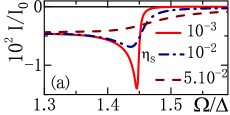
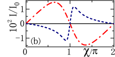
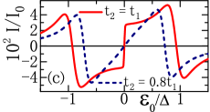
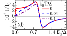
Figure 5: (Color online). (a) $\eta_{s}$-broadening of the ABS-to-gap edge resonance at $\varphi=0$: same parameters as in Fig. 4a with $t_{1}=t_{2}$. (b) Dependence on $\chi$ ($\varphi=0$), with $\varepsilon_{0}=0.1\Delta$, $t_{1}=t_{2}=0.6\Delta$, $b_{1}=b_{2}=0.2$ and $\Omega=0.85\Delta$ (red dot-dashed, close to an extremum in $\Omega$) or $\Omega=0.9\Delta$ (blue dashed, close to the resonance center). (c) Dependence on $\varepsilon_{0}$ ($\varphi=\pi,\chi=\frac{\pi}{2}$), with $\Omega=0.6\Delta$, $t_{1}=\Delta$, $t_{2}=t_{1}$ or $t_{2}=0.8t_{1}$, $b_{1}=b_{2}=0.2$. (d) Temperature dependence (same as (c), $t_{2}=t_{1}$).

Let us comment in more detail on the vicinity of a resonance such that $n\Omega\sim 2E_{A}(\varphi)$, with $\pm E_{A}(\varphi)$ the equilibrium Andreev bound state energies. The salient result, featured in Fig. 4, is the maximal chiral current close to the resonance, and its rapid sign change as the resonance is crossed. The exact calculation qualitatively agrees well with the RWA calculation in the IGM (Section IIIC). This is illustrated in Figure 6. No quantitative agreement is possible due to the renormalizing effect of the quasiparticles. Yet, except for the resonance towards the continuum, one can nearly match the results of the Keldysh calculation with the IGM by fitting the parameters of the latter.

The resonant chiral pumping effect found above is robust against nonzero temperature ($k_{B}T=0.1\Delta$ here) and junction asymmetry (Fig. 5c), and also nonsymmetric microwave amplitudes (Fig. 4c, d). It bears some similarity with pumping mechanisms, as explored in a variety of situations with normal or superconducting islandsresonant_pumping. Yet, it is remarkable that the chiral current emerges only beyond the adiabatic regime and is maximal if the microwave frequency – or its harmonics – matches the ABS spacing, which is precisely an antiadiabatic effect. For small $\varepsilon_{0}$, the resonant chiral current is larger at $\varphi=\pi$ than at $\varphi=0$, due to the nonharmonicity of the equilibrium $I(\varphi)$ close to $\varphi=\pi$.

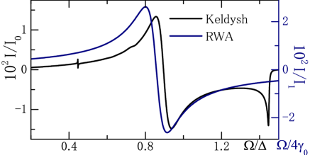
Figure 6: (Color online) Chiral current at $\varphi=0$, $\chi=\frac{\pi}{2}$ close to the first harmonic resonance. Keldysh result ($\varepsilon_{0}=0.2\Delta$, $t_{1}=t_{2}=1.0\Delta$, $b_{1}=b_{2}=0.2$) vs RWA (infinite gap) with fitted parameters $\gamma_{0}=1.0$, $b=0.2$, $\epsilon_{0}=0.8$.

Fig. 7 shows the frequency dependence of the chiral current for a stronger microwave amplitude ($b_{1}=b_{2}=1.2$). The resonances are much broader, and above all, very sizeable chiral currents are obtained, close to $0.8I_{0}$ for $\varphi=\pi$.

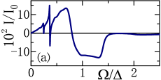
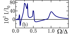
Figure 7: (Color online). (a) Variation with $\Omega$ of the chiral current ($\varphi=0$, $\chi=\frac{\pi}{2}$), with $\varepsilon_{0}=0.1\Delta$, $t_{1}=t_{2}=0.6\Delta$, $b_{1}=b_{2}=1.2$ (b) Same but $\varphi=\pi$.

The $\chi$-dependence of the chiral current can be compared to the $\varphi$-dependence of the junction equilibrium current (e.g. with no microwave). The microwave amplitude conspires with the junction transparency to control the current amplitude far from resonance. This is similar to an equilibrium junction with a non resonant dot. Indeed, the $\sin\chi$ variation resembles the $\sin\varphi$ variation obtained for a nonresonant dot. On the other hand, at a maximum close to resonance, the strongly nonharmonic $\sin\frac{\chi}{2}$ variation (for $\varphi=0$) resembles that obtained for a symmetric resonant dot junction if $\varepsilon_{0}=0$: there, closure of the Andreev gap at $\varphi=\pi$ results in a sawtooth jump of the equilibrium current at zero temperature, which is rounded by asymmetry and temperature (Fig. 5). A similar situation is met in the chiral case, with a nonzero $\varepsilon_{0}$ but chiral microwave resonant with the ABS spacing. While in the non-resonant case the $\chi$ variation goes like $\sin\chi$, in the resonant regime it approaches $|\sin\frac{\chi}{2}|$. This interpretation is confirmed by the asymmetry and temperature rounding of the jump at $\varepsilon_{0}=0$ (Eq. 38 and Fig. 5c, d). Moreover, the change of sign in $I_{chir}(\chi)$ upon crossing resonance can be compared to the change of an equilibrium $I(\varphi)$ from $0$ to $\pi$ character.

For stronger microwave amplitudes, the current-phase relation is strongly anharmonic and the resonances much broaderBergeret1 ; Bergeret2 , and the same is true for the chiral current.

Also, a chiral current persists in presence of cross-talk between the two dephased microwave excitations and towards the dot gate.This can be shown by setting, instead of Eq. (1), $\varphi_{1}=\frac{\varphi}{2}+b_{1}\cos(\Omega t+\frac{\chi}{2})+b^{\prime}_{1}\cos(\Omega t-\frac{\chi}{2})$, $\varphi_{2}=-\frac{\varphi}{2}+b_{2}\cos(\Omega t-\frac{\chi}{2})+b^{\prime}_{2}\cos(\Omega t+\frac{\chi}{2})$, $\varepsilon_{0}(t)=\varepsilon_{0}+\varepsilon_{1}\cos(\Omega t+\frac{\chi}{2})+\varepsilon_{2}\cos(\Omega t-\frac{\chi}{2})$. Generalizing the large-$\Omega$ calculation, one obtains (Appendix C):

$$I_{chir}=\pm\frac{2e}{\hbar^{2}}\frac{\gamma_{1}\gamma_{2}(b_{1}b_{2}-b^{\prime}_{1}b^{\prime}_{2})\varepsilon_{0}\sin\chi}{\Omega E_{0}^{eff}}$$ (58)

where $E_{0}^{eff}$ is an effective ABS energy depending on the dot level modulations $\varepsilon_{1,2}$. The chiral current is thus robust against small crosstalk $b^{\prime}_{1,2}\neq 0$.

V Lattice chain mapping

The Cooper pair pumping mechanism, illustrated in the IGM, can be understood in relation with charge pumping in some tight-binding chain models. For this purpose, let us introduce the number state representation $|N,\nu\rangle$ where $N$ is the number of pairs exchanged through the junction from terminal $1$ to terminal $2$, and $\nu=0,1$ indicates the charge state of the dot. The variable $N$ is by convention defined here from the pair numbers $N_{1,2}$ by $N=\frac{N_{2}-N_{1}-\nu}{2}$. The variable $N$ is conjugated of the superconducting phase difference $\varphi$. As a result, it is straightforward to rewrite the Hamiltonian $H_{\infty}$ in the number basis as:

$$H_{\infty}=\sum_{N}\varepsilon_{0}\big{(}|N,1\rangle\langle N,1|-|N,0\rangle\langle N,0|\big{)}+\sum_{N}\big{(}\gamma_{1}e^{-i\varphi_{1}(t)}|N,1\rangle\langle N,0|+\gamma_{2}e^{-i\varphi_{2}(t)}|N-1,1\rangle\langle N,0|+H.c.\big{)}$$ (59)

The above convention means that transferring a pair from terminal $1$ to the dot does not change $N$ while transfering this pair from the dot to terminal $2$ increases $N$ by $1$. This maps the IGM on a bipartite tight-binding chain, described by a model of the class of Rice-Mele modelsRice-Mele . The sites of this chain are indexed by $(N,\nu)$ and the phase $\varphi$ plays the role of the one-dimensional wavevector $k$ and both models yield the two-level Hamiltonian given by Equation 10. The comparison with Rice-Mele model is more transparent in the limit $b<<1$ where the time dependence is harmonic and one has $H_{\infty}(t)=\vec{h}(t).\vec{\sigma}$ with

$$\vec{h}(t)=\Big{(}(\gamma_{1}+\gamma_{2})\cos\frac{\varphi}{2}-(\gamma_{1}\delta\varphi_{1}(t)-\gamma_{2}\delta\varphi_{2}(t))\sin\frac{\varphi}{2},(\gamma_{1}-\gamma_{2})\sin\frac{\varphi}{2}+(\gamma_{1}\delta\varphi_{1}(t)+\gamma_{2}\delta\varphi_{2}(t))\cos\frac{\varphi}{2},\varepsilon_{0}\Big{)}$$ (60)

with $\delta\varphi_{1,2}(t)=b_{1,2}\cos(\omega t\pm\frac{\chi}{2})$. Notice that in absence of microwave excitation, the IGM maps onto a SSH model.

The existence of pumped charge current in such models, as proposed and realized in experimentspumping1 ; pumping2 , provides an interpretation of our results. An interesting point is that due to the presence of a continuum of quasiparticle states, the full model described by Equation 10 goes well beyond such a simple chain model. This work shows that the pumping properties are robust against the incorporation of such continuum states. Moreover, pumping scenarios are usually considered in the quasi-adiabatic limitThouless , while here, we have studied the full frequency range and new resonant features.

VI Conclusion

In conclusion, this work demonstrates that two dephased microwave fields microwaves provide nonadiabatic pumping of Josephson currents without any superconducting phase difference. The current is driven by the microwave phase $\chi$ and is tuned in amplitude and sign by crossing ABS resonances. The chirality has its root in the structure of the wavefunction of the ABS as a function of two phases ($\varphi_{1}(t)$ and $\varphi_{2}(t)$, or equivalently $\varphi$ and $\Omega t$). The chiral properties are robust against temperature and asymmetry in the junction parameters ($\gamma_{1}\neq\gamma_{2}$) and in the microwave amplitudes. Most results have been shown with small microwave amplitudes, but larger values of $I_{chir}$ comparable to $I_{0}$ can be easily be reached in experiments. The striking sign change of the current at resonance contrasts with the current amplitude minima found in the nonchiral caseBergeret1 ; Bergeret2 . All the possible known regimes of current in a standard Josephson junction (harmonic or sawtooth phase dependence, “$0$” or “$\pi$” junction, as well as very anharmonic ones like in $\varphi_{0}$-junctions) are encountered for the chiral current as a function of $\chi$. Using an electrostatic gate or tuning the microwave frequency offers a fine control of the chiral current, in amplitude and sign. The latter resulting from symmetry properties, Coulomb interactions are not expected to change qualitatively the physics.

In a Josephson transistorJTransistor , the current amplitude oscillates with the gate without any sign change as the dot levels pass across the gap. Due to the additional gate-controlled sign change, the proposed set-up deserves the name of chiral Josephson transistor. A generalization to a multilevel dot is possible but involving also microwave transitions between different channel ABS. Also, the chiral current variation quadratic with the microwave amplitude recalls the photogalvanic effect studied in Ref. Grushin, .

D. F. gratefully acknowledges fruitful discussions with C. Balseiro and G. Usaj.

Appendix A Rotating Wave Approximation

The general form of the $\hat{H}_{n}(t)$ matrix in Equation (46) is the following:

$$\hat{H}_{n}(t) =\hat{\tau}_{z}\left[E_{A}+\dot{\beta}\cos^{2}\frac{\theta}{2}-\frac{\dot{\beta}+\dot{\alpha}}{2}+\eta\sin\theta\partialderivative{|\Gamma|}{\varphi}-n\frac{\Omega}{2}\right]$$ (61)

$$+\hat{\tau}_{x}\left[\eta\cos\theta\cos\alpha\partialderivative{|\Gamma|}{\varphi}\cos(n\Omega t)-\left(\frac{\dot{\theta}}{2\cos\alpha}+\eta\cos\theta\sin\alpha\partialderivative{|\Gamma|}{\varphi}\right)\sin(n\Omega t)\right]$$

$$+\hat{\tau}_{y}\left[-\left(\frac{\dot{\theta}}{2\cos\alpha}+\eta\cos\theta\sin\alpha\partialderivative{|\Gamma|}{\varphi}\right)\cos(n\Omega t)-\eta\cos\theta\cos\alpha\partialderivative{|\Gamma|}{\varphi}\sin(n\Omega t)\right]$$

$$+\frac{\dot{\beta}+\dot{\alpha}}{2}.$$

We consider the cases $\varphi=0$ $(\zeta=1)$ and $\pi$ $(\zeta=-1)$:

$$|\Gamma(t)|=\sqrt{2\gamma_{0}^{2}\left(1+\zeta\cos(2b\sin\Omega t\sin\frac{\chi}{2})\right)}$$ (62)

$$\partialderivative{|\Gamma(t)|}{\varphi}=-\frac{\zeta\gamma_{0}^{2}}{|\Gamma(t)|}\sin(2b\sin\Omega\sin\frac{\chi}{2})$$ (63)

$$E_{A}(t)=\sqrt{\epsilon_{0}^{2}+|\Gamma(t)|^{2}}$$ (64)

$$\dot{\beta}=\Omega b\sin\Omega t\cos\frac{\chi}{2}$$ (65)

$$\cos[\theta(t)]=\frac{\epsilon_{0}}{E_{A}(t)}$$ (66)

$$\sin[\theta(t)]=\frac{|\Gamma(t)|}{E_{A}(t)}$$ (67)

$$\tan[\alpha(t)]=-\frac{\dot{\beta}\sin\theta}{\dot{\theta}}.$$ (68)

Let us first consider $\varphi=0$, with $b$ small. Taylor expanding the expression of $\tan\alpha$ in Eq. (68) leads to

$$(\tan[\alpha(t)])^{-1}=\frac{\epsilon_{0}}{E_{0}}b\frac{\sin^{2}\frac{\chi}{2}}{\cos\frac{\chi}{2}}\cos\Omega t,$$ (69)

meaning that $(\tan[\alpha(t)])^{-1}$ is not small if $\chi$ is close to $\pi$. Imposing time-continuity of $\alpha$ implies $\sin\alpha>0$. Therefore $\sin\alpha=\frac{1}{f(t)}$ where $f(t)=\sqrt{1+\frac{\epsilon_{0}^{2}}{E_{0}^{2}}b^{2}\cos^{2}\Omega t\frac{\sin^{4}\frac{\chi}{2}}{\cos^{2}\frac{\chi}{2}}}$ and $\cos\alpha=\frac{\epsilon_{0}}{E_{0}}b\frac{\sin^{2}\frac{\chi}{2}}{\cos\frac{\chi}{2}}\cos\Omega t/f(t)$. Using the first harmonic $n=1$, Taylor expanding and integrating, Eq. (47) yield Equation (III.4) where $F_{1},F_{2}$ are defined by

$$F_{1}=\frac{\int_{0}^{T}\sin^{2}\Omega tf(t)}{\int_{0}^{T}\sin^{2}\Omega t}\,,\quad F_{2}=\frac{\int_{0}^{T}\sin^{2}\Omega t/f(t)}{\int_{0}^{T}\sin^{2}\Omega t}.$$ (70)

A similar calculation in the case $\varphi=\pi$ makes use of

$$G_{1}=\frac{\int_{0}^{T}\left|\sin 2\Omega t\right|g_{1}(t)}{\int_{0}^{T}\left|\sin 2\Omega t\right|}\,,\quad G_{2}=\frac{\int_{0}^{T}\left|\sin\Omega t\right|\sin^{2}\Omega t/g_{2}(t)}{\int_{0}^{T}\left|\sin\Omega t\right|\sin^{2}\Omega t},$$

with

$$g_{1}(t)=\sqrt{1+b^{2}\cos^{2}\frac{\chi}{2}\frac{\sin^{4}\Omega t}{\cos^{2}\Omega t}}\,,\quad g_{2}(t)=\left|\cos\Omega t\right|g_{1}(t).$$ (72)

Appendix B Green’s functions

Let us define the bare Green’s functions (GFs) and the tunnel self-energy for the calculation of the current.

$$\Sigma_{jd}^{R,A}=\begin{pmatrix}t_{j}e^{i\varphi_{j}(t)/2}&0\\ 0&-t_{j}e^{-i\varphi_{j}(t)/2}\end{pmatrix}$$ (73)

($j=1,2$). The bare GFs in the leads are given by

$$\hat{g}^{r,a}_{jj}=\frac{\pi\nu(0)}{\sqrt{\Delta^{2}-(\omega\pm i\eta_{s})^{2}}}\begin{pmatrix}-(\omega\pm i\eta_{s})&\Delta\\ \Delta&-(\omega\pm i\eta_{s})\end{pmatrix}$$ (74)

and $\hat{g}^{+-}_{jj}(\omega)=n_{F}(\omega)\big{(}\hat{g}^{A}_{jj}(\omega)-\hat{g}^{R}_{jj}(\omega)\big{)}$.

The bare GFs in the dot are given by $\hat{g}^{R,A}_{dd}=(\omega-\varepsilon_{0}\hat{\tau}_{z}\pm i\eta_{d})^{-1}$ and $\hat{g}^{+-}_{dd}(\omega)=n_{F}(\omega)\big{(}\hat{g}^{a}_{dd}(\omega)-\hat{g}^{r}_{dd}(\omega)\big{)}$. The broadening parameters $\eta_{s},\eta_{d}$ mimic residual inelastic processes.

Expanding the Dyson equation (IV) yields

$$G_{d1}^{+-}= (1+G_{dd}^{r}\Sigma_{d1}^{r}g_{11}^{r}\Sigma_{1d}^{r}+G_{dd}^{r}\Sigma_{d2}^{r}g_{22}^{r}\Sigma_{2d}^{r})g_{dd}^{+-}(\Sigma_{d1}^{a}g_{11}^{a}+\Sigma_{d1}^{a}g_{11}^{a}\Sigma_{1d}^{a}G_{dd}^{a}\Sigma_{d1}^{a}g_{11}^{a}+$$ (75)

$$\Sigma_{d2}^{a}g_{22}^{a}\Sigma_{2d}^{a}G_{dd}^{a}\Sigma_{d1}^{a}g_{11}^{a})$$

$$+G_{dd}^{r}\Sigma_{d1}^{r}g_{11}^{+-}(1+\Sigma_{1d}^{a}G_{dd}^{a}\Sigma_{d1}^{a}g_{11}^{a})+G_{dd}^{r}\Sigma_{d2}^{r}g_{22}^{+-}\Sigma_{2d}^{a}G_{dd}^{a}\Sigma_{d1}^{a}g_{11}^{a}$$

$$G_{1d}^{+-}= (g_{11}^{r}\Sigma_{1d}^{r}+g_{11}^{r}\Sigma_{1d}^{r}G_{dd}^{r}\Sigma_{d1}^{r}g_{11}^{r}\Sigma_{1d}^{r}+g_{11}^{r}\Sigma_{1d}^{r}G_{dd}^{r}\Sigma_{d2}^{r}g_{22}^{r}\Sigma_{2d}^{r})g_{dd}^{+-}(1+\Sigma_{d1}^{a}g_{11}^{a}\Sigma_{1d}^{a}G_{dd}^{a}+$$ (76)

$$\Sigma_{d2}^{a}g_{22}^{a}\Sigma_{2d}^{a}G_{dd}^{a})$$

$$+(1+g_{11}^{r}\Sigma_{1d}^{r}G_{dd}^{r}\Sigma_{d1}^{r})g_{11}^{+-}\Sigma_{1d}^{a}G_{dd}^{a}+g_{11}^{r}\Sigma_{1d}^{r}G_{dd}^{r}\Sigma_{d2}^{r}g_{22}^{+-}\Sigma_{2d}^{a}G_{dd}^{a},$$

where $G_{dd}^{r,a}$ is the full retarded or advanced Green’s function localized on the dot such as

$$G_{dd}^{r,a}=((g_{dd}^{r,a})^{-1}-(\Sigma_{d1}g_{11}^{r,a}\Sigma_{1d}+\Sigma_{d2}g_{22}^{r,a}\Sigma_{2d}))^{-1}.$$ (77)

Here $\Sigma_{dj,n}$ (respectively $\Sigma_{jd,n}$) is the $n$th harmonic of the self-energy defined in Eq. 73.

$$\Sigma_{d1,n}=\Sigma^{*}_{1d,-n}=\begin{pmatrix}t_{1}e^{-i\varphi/4}(-i)^{n}J_{n}(\frac{b_{1}}{2})e^{in\chi/2}&0\\ 0&-t_{1}e^{i\varphi/4}i^{n}J_{n}(\frac{b_{1}}{2})e^{in\chi/2}\end{pmatrix}$$

$$\Sigma_{d2,n}=\Sigma^{*}_{2d,-n}=\begin{pmatrix}t_{2}e^{i\varphi/4}(-i)^{n}J_{n}(\frac{b_{2}}{2})e^{-in\chi/2}&0\\ 0&-t_{2}e^{-i\varphi/4}i^{n}J_{n}(\frac{b_{2}}{2})e^{-in\chi/2}\end{pmatrix}.$$ (78)

Appendix C Crosstalk effects

Let us consider the infinite gap model Hamiltonian with crosstalk between the microwave amplitudes (and phases) applied on superconductors $1,2$, and towards the electrostatic gate:

$$H_{\infty}(t)=\begin{pmatrix}\epsilon&\Gamma(t)\\ \Gamma^{*}(t)&-\epsilon\end{pmatrix},$$ (79)

with $\Gamma(t)=\sum_{j=1,2}\gamma_{j}e^{-i\varphi_{j}(t)}$, and:

$$\varphi_{1} =\frac{\varphi}{2}+b_{1}\cos(\Omega t+\frac{\chi}{2})+b_{1}^{\prime}\cos(\Omega t-\frac{\chi}{2})$$

$$\varphi_{2} =-\frac{\varphi}{2}+b_{2}\cos(\Omega t-\frac{\chi}{2})+b_{2}^{\prime}\cos(\Omega t+\frac{\chi}{2})$$

$$\epsilon =\epsilon_{0}+\epsilon_{1}\cos(\Omega t+\frac{\chi}{2})+\epsilon_{2}\cos(\Omega t-\frac{\chi}{2}),$$ (80)

with $b_{j},b_{j}^{\prime},\epsilon_{j}>0$. The crosstalk from superconductor $1$ to $2$ ($2$ to $1$) is described by the terms $b^{\prime}_{1,2}$ and the crosstalk with the gate voltage applied to the dot is described by $\varepsilon_{1,2}$. Using only the first harmonics in the Fourier decomposition of the Hamiltonian defined in Eq. (79) leads to

$$H_{\infty}(t)=\tilde{H}_{\infty 0}+\tilde{H}_{\infty 1}e^{i\Omega t}+\tilde{H}_{\infty-1}e^{-i\Omega t},$$ (81)

Using Brillouin-Wigner perturbation theory, the effective Hamiltonian becomes

$$H_{\infty eff}=\tilde{H}_{\infty 0}+\frac{1}{\Omega}[\tilde{H}_{\infty 1},\tilde{H}_{\infty-1}],$$ (82)

and after a straightforward calculation, its eigenvalues are found to be:

$$E^{2}_{\varphi}= \,\,\tilde{\epsilon}^{2}+\gamma_{1}^{2}+\gamma_{2}^{2}+2\gamma_{1}\gamma_{2}\cos\varphi$$

$$-\cos\chi\left[\gamma_{1}^{2}b_{1}b_{1}^{\prime}+\gamma_{2}^{2}b_{2}b_{2}^{\prime}+\gamma_{1}\gamma_{2}\cos\varphi\left(b_{1}b_{1}^{\prime}+b_{2}b_{2}^{\prime}\right)\right]$$

$$-\frac{2\sin\chi}{\Omega}\left[\gamma_{1}^{2}B_{1}^{2}+\gamma_{2}^{2}B_{2}^{2}+\gamma_{1}\gamma_{2}\cos\varphi\left(B_{1}+B_{2}\right)\right]$$

$$+\frac{\sin^{2}\chi}{\Omega^{2}}\left[\gamma_{1}^{2}B_{1}^{2}+\gamma_{2}^{2}B_{2}^{2}\right]+2\frac{\gamma_{1}\gamma_{2}}{\Omega^{2}}\cos\varphi B_{1}B_{2}\sin^{2}\chi.$$ (83)

where $\tilde{\epsilon}=\epsilon_{0}+\gamma_{1}\gamma_{2}\sin\varphi\sin\chi[b_{1}b_{2}-b_{1}^{\prime}b_{2}^{\prime}]$, $B_{1}=b_{1}\epsilon_{2}-b_{1}^{\prime}\epsilon_{1}$, and $B_{2}=b_{2}^{\prime}\epsilon_{2}-b_{2}\epsilon_{1}$. Thisleads to the DC-current at $\varphi=0,\,\pi$:

$$I_{\varphi=0,\pi}=2e\frac{\gamma_{1}\gamma_{2}\epsilon_{0}\sin\chi\left(b_{1}b_{2}-b_{1}^{\prime}b_{2}^{\prime}\right)}{\Omega E_{0}^{eff}},$$ (84)

where $E_{0}^{eff}=E_{\varphi=0,\pi}$ as given by (83).

References

• (1) A. Barone, G. Paternó, Physics and Applications of the Josephson Effect (Wiley, Interscience, New York, 1982).
• (2) A. H. Dayem and R.J. Martin, Phys. Rev. Lett. 8, 246 (1962)
• (3) P. K. Tien and J.P. Gordon, Phys. Rev. 129, 647 (1963).
• (4) S. Shapiro, Phys. Rev. Lett. 11, 80 (1963).
• (5) C. W. J. Beenakker and H. van Houten, Phys. Rev. Lett. 66, 3056 (1991); A. Furusaki and M. Tsukada, Solid Sate Comm. 78, 299 (1991).
• (6) F. S. Bergeret, P. Virtanen, T. T. Heikkilä, and J. C. Cuevas, Phys. Rev. Lett. 105, 117001 (2010).
• (7) F. S. Bergeret, P. Virtanen, A. Ozaeta, T. T. Heikkilä, and J. C. Cuevas, Phys. Rev. B 84, 054504 (2011).
• (8) L. Bretheau, Ç. Girit, H. Pothier, D. Esteve, and C. Urbina, Nature 499, 7458 (2013).
• (9) D. J. Thouless, Phys. Rev. B 27, 6083 (1983).
• (10) Q. Niu, Phys. Rev. Lett. 64.
• (11) H. Pothier, P. Lafarge, C. Urbina, D. Esteve, and M. H. Devoret, Europhys. Lett. 17, 249 (1992).
• (12) N. B. Kopnin, A. S. Mel’nikov, and V. M. Vinokur, Phys. Rev. Lett. 96, 146802 (2006).
• (13) F. Taddei, M. Governale, and R. Fazio, Phys. Rev. B 70, 052510 (2004); F. Giazotto, P. Spathis, S. Roddaro, S. Biswas, F. Taddei, M. Governale, and L. Sorba, Nat. Phys. 7, 857 (2011).
• (14) S. Russo, J. Tobiska, T. M. Klapwijk, and A. F. Morpurgo, Phys. Rev. Lett. 99, 086601 (2007).
• (15) L. N. Bulaevskii, V. V. Kuzii, and A. A. Sobyanin, Solid State Commun. 25, 1053 (1978).
• (16) I. V. Krive, A. M. Kadigrobov, R. I. Shekhter, and M. Jonson, Phys. Rev. B 71 214516 (2005).
• (17) A. Zazunov, R. Egger, T. Jonckheere, and T. Martin, Phys. Rev. Lett. 103, 147004 (2009).
• (18) A. A. Reynoso, G. Usaj, C. A. Balseiro, D. Feinberg, and M. Avignon, Phys. Rev. Lett. 101, 107001 (2008).
• (19) A. I. Buzdin, Phys. Rev. Lett. 101, 107005 (2008).
• (20) J-F. Liu and K. S. Chan, Phys. Rev. B 82, 125305 (2010).
• (21) H. Sickinger, A. Lipman, M. Weides, R. G. Mints, H. Kohlstedt, D. Koelle, R. Kleiner, and E. Goldobin, Phys. Rev. Lett. 109, 107002 (2012).
• (22) T. Yokohama, M. Eto, and Yu V. Nazarov, Phys. Rev. B 89, 195407 (2014).
• (23) D. B. Szombati, S. Nadj-Perge, D. Car, R. Plissard, E. P. A. M. Bakkers, and L. P. Kouwenhoven, Nat. Phys. 12, 568 (2016).
• (24) M. Grifoni and P. Hänggi, Phys. Rep. 304, 229 (1998).
• (25) Xiao, D., Chang, M. and Niu, Q. (2010). Berry phase effects on electronic properties. Reviews of Modern Physics, 82(3), pp.1959-2007.
• (26) T. Jonckheere, A. Zazunov, K. V. Bayandin, V. Shumeiko, and T. Martin, Phys. Rev. B80, 184510 (209).
• (27) T. Mikami, S. Kitamura, K. Yasuda, N. Tsuji, T. Oka, and H. Aoki, Phys. Rev. B 93, 144307 (2016).
• (28) P. Jarillo-Herrero, J. A. van Dam and L. P. Kouwenhoven, Nature 439, 953 (2006).
• (29) L. P. Kouwenhoven, S. Jauhar, K. McCormick, D. Dixon, P. L. McEuen, Yu. V. Nazarov, N. C. van der Vaart, and C. T. Foxon, Phys. Rev. B 50, 2019 (1994).
• (30) This argument easily generalizes to the solution of the full model (Hamiltonian (II)), by oberving that the current is given by the derivative of the full free energy, including quasiparticles, and that in the adiabatic approximation, the latter is a function of the phase $\varphi_{1}(t)-\varphi_{2}(t)$ only.
• (31) M. Z. Hasan and C. L. Kane, Rev. Mod. Phys. 82, 3045 (2010).
• (32) C. Caroli, R. Combescot, P. Nozières and D. Saint-James, J. Phys. C 4, 916 (1971).
• (33) J. C. Cuevas, A. Martín-Rodero, and A. Levy Yeyati, Phys. Rev. B 54, 7366 (1996).
• (34) R. Mélin and S. Peysson, Phys. Rev. B 68, 174515 (2003).
• (35) J.D. Pillet, C. Quay, P. Morfin, C. Bena, A. Levy Yeyati and P. Joyez, Nature Physics 6, 965 (2010).
• (36) R. Mélin, J. G. Caputo, K. Yang and B. Douçot, Phys. Rev. B 95, 085415 (2017).
• (37) M. J. Rice and E. J. Mele, Phys. Rev. Lett. 49, 1455 (1982).
• (38) S. Nakajima, T. Tomita, Shintaro Taie, T. Ichinose, H. Ozawa, L. Wang, M. Troyer and Y. Takahashi, Nat. Phys. 12, 296 (2016).
• (39) M. Lohse, C. Schweizer, O. Zilberberg, M. Aidelsburger, and I. Bloch, Nat. Phys. 12, 350 (2016).
• (40) F. de Juan, A. G. Grushin, T. Morimoto, and J. E. Moore, Nat. Commun. 8, 15995 (2017).