Numerical Calculation of the Complex Berry Phase in Non-Hermitian Systems

Abstract

We numerically investigate topological phases of periodic lattice systems in tight-binding description under the influence of dissipation. The effects of dissipation are effectively described by $\mathcal{PT}$-symmetric potentials. In this framework we develop a general numerical gauge smoothing procedure to calculate complex Berry phases from the biorthogonal basis of the system’s non-Hermitian Hamiltonian. Further, we apply this method to a one-dimensional $\mathcal{PT}$-symmetric lattice system and verify our numerical results by an analytical calculation.

1 Introduction

Due to their robustness against local defects or disorder topologically protected states as Majorana fermions [1, 2, 3] are of high value for physical applications such as quantum computation [4]. However, no physical system is completely isolated and dissipation can have an important influence on the states [5]. Majorana fermions can even be created with the help of dissipative effects [6, 7].

Of special importance in this context is the case of balanced gain and loss as described by $\mathcal{PT}$-symmetric complex potentials [8], which has attracted large interest in quantum mechanics [9, 10, 11, 12, 13]. The stationary Schrödinger equation was solved for scattering solutions [14] and bound states [15], and also questions concerning other symmetries [16, 17] as well as the meaning of non-Hermitian Hamiltonians have been discussed [18, 19]. Their influence on many-particle systems has been studied mainly in the context of Bose-Einstein condensates [20, 21, 22, 23, 24, 25] but also on lattice systems [26, 27, 28, 29, 30, 31]. In the latter systems it was shown that $\mathcal{PT}$-symmetric complex potentials may eliminate the topologically protected states existing in the same system under complete isolation [26, 27, 28, 29, 30, 32, 33]. However, in some $\mathcal{PT}$-symmetric potential landscapes they can survive [28, 29, 30, 31, 32, 34], which has been confirmed in impressive experiments [33, 35]

In most theoretical studies the topologically protected states have been identified via their property to close the energy gap of the band structure or their localisation at edges or interfaces of the systems [26, 32, 28, 29, 30]. The identification and calculation of topological invariants such as the Zak phase [36] known from Hermitian systems leads to new challenges in the case of non-Hermitian operators [27, 37, 38]. This is especially true if the eigenstates are only available numerically. Indeed, in Refs. [27, 37, 38] all calculations have been done for eigenstates which are analytically available. However, for arbitrary $\mathcal{PT}$-symmetric complex potentials analytical access to the eigenstates is not available and a reliable numerical procedure is required. For the calculation of the invariants an integration of phases over a loop in parameter space is typically necessary.

For example, in the case of the Zak phase, which is applied to one-dimensional systems, this integral runs over the first Brillouin zone. The integrand contains the eigenstates of the Hamiltonian and their first derivatives. In a numerical calculation it is evaluated at discrete points in momentum space and each state possesses an arbitrary global phase spoiling the phase relation.

This is the point our study sets in. In this article we introduce a robust method of calculating the complex Berry phase numerically. It is based on a normalisation of the left- and right-hand eigenvectors with the biorthogonal inner product [39], which reduces to the c product [40] in the case of complex symmetric Hamiltonians. To obtain an unambiguous complex Berry phase we introduce a numerical gauge smoothing procedure. It consists of two parts. First we have to remove the influence of the arbitrary and unconnected global phases of the eigenstates, which is unavoidably attached to them for each point in parameter space. This is achieved by relating the eigenvectors of consecutive steps in parameter space, and then normalising them. With this approach the eigenvectors are not yet single-valued, i.e. the vectors at the starting and end point of the loop possess different phases. These points have to be identified and will be refered as the basepoint of the loop later on. The phase difference between the different left and right states at the basepoint has to be corrected by ensuring the eigenvectors to be identical at the basepoint.

The article is organised as follows. First, we introduce the complex Berry phase in section 2. In section 3 we establish the algorithm of the gauge smoothing procedure for non-Hermitian (and Hermitian) Hamiltonians. An example is presented in section 4, where we apply the previously developed method to a non-Hermitian extension of the Su-Schrieffer-Heeger (SSH) model [41] to calculate its complex Zak phase.

2 Complex Berry phase

Topological phases of closed one-dimensional periodic lattice systems are characterised by the Zak phase [36], which is the Berry phase [42] picked up by the eigenstate when it is transported once along the Brillouin zone. In the presence of an antiunitary symmetry these phases are quantised [43] and can be related to the winding number of a vector $\boldsymbol{n}(k)$ determining the Bloch Hamiltonian

$$\mathcal{H}(k)=\boldsymbol{n}(k)\cdot\boldsymbol{\sigma}\;,$$ (1)

where $\boldsymbol{\sigma}$ denotes the vector of Pauli matrices and $k$ is the wave number parametrising the Brillouin zone, which acts as parameter space. In this case the Zak phase characterises the system’s topological phase.

This concept can be generalised to dissipative systems effectively described by a $\mathcal{PT}$-symmetric non-Hermitian Hamiltonian $H(\boldsymbol{\alpha})$. The complex Berry phase $\gamma_{n}$ of a biorthogonal pair of eigenvectors $\langle\chi_{n}|$ and $|\phi_{n}\rangle$ of $H(\boldsymbol{\alpha})$,

$$\gamma_{n}=\mathrm{i}\oint\limits_{\mathcal{C}}\,\langle\chi_{n}|\boldsymbol{\nabla}_{\boldsymbol{\alpha}}|\phi_{n}\rangle\cdot\mathrm{d}\boldsymbol{\alpha}\;,$$ (2)

follows from the lowest order of the adiabatic approximation of the time evolution of a state in parameter space [44]. Here $\mathcal{C}$ is a loop in parameter space and $\boldsymbol{\alpha}=(\alpha_{1},...,\alpha_{i},...)$ are its coordinates. We consider $\mathcal{PT}$-symmetric non-Hermitian Hamiltonians of the form

$$H(\boldsymbol{\alpha})=H_{\text{h}}(\boldsymbol{\alpha})+H_{\text{nh}}(\boldsymbol{\alpha})\;,$$ (3)

where $H_{\text{h}}$ denotes its Hermitian and $H_{\text{nh}}$ represents its $\mathcal{PT}$-symmetric non-Hermitian part. The non-Hermitian part is a complex potential modelling the gain and loss of particles.

The complex Berry phase $\gamma_{n}$ arising from the periodic modulation of states in the parameter space of a $\mathcal{PT}$-symmetric one-dimensional system cannot be related to a real winding number calculated from eq. (1). Hence, the calculation of the complex Berry phase requires the determination of gauge-smoothed eigenvector pairs along the loop $\mathcal{C}$ in parameter space allowing for the evaluation of eq. (2).

Here, it is important to note that the argumentation of Hatsugai [43] for the quantisation of Berry phases of Hermitian Hamiltonians can be extended on complex Berry phases of non-Hermitian $\mathcal{PT}$-symmetric Hamiltonians in the case of unbroken $\mathcal{PT}$ symmetry. One finds the real part of the complex Berry phase to take values $0$ or $\pi$ modulo $2\pi$. Thus, a strict quantisation is still present and the $\mathcal{PT}$ symmetry protects the topological phases occurring in such systems.

3 Numerical gauge smoothing

In this section we present a numerical procedure to determine the left and right eigenvectors $\langle\chi_{n}|$ and $|\phi_{n}\rangle$ in an appropriate smoothed gauge to compute complex Berry phases on a discretised loop $\mathcal{C}=(\boldsymbol{\alpha}_{1},...,\boldsymbol{\alpha}_{j},...,\boldsymbol{\alpha}_{M}=\boldsymbol{\alpha}_{1})$ in parameter space. This is necessary for the evaluation of integrals of the form in eq. (2). Typically the left and right eigenvectors have to be calculated independently, and each of them has an arbitrary global phase. The biorthogonal normalisation condition [39],

$$\langle\chi_{n}(\boldsymbol{\alpha}_{j})|\rightarrow \,\frac{\langle\chi_{n}(\boldsymbol{\alpha}_{j})|}{\sqrt{\langle\chi_{n}(\boldsymbol{\alpha}_{j})|\phi_{n}(\boldsymbol{\alpha}_{j})\rangle}}\;,$$ (4a)

$$|\phi_{n}(\boldsymbol{\alpha}_{j})\rangle\rightarrow \,\frac{|\phi_{n}(\boldsymbol{\alpha}_{j})\rangle}{\sqrt{\langle\chi_{n}(\boldsymbol{\alpha}_{j})|\phi_{n}(\boldsymbol{\alpha}_{j})\rangle}}\;,$$ (4b)

chooses one arbitrary global phase for each $\boldsymbol{\alpha}_{j}$. This is sufficient if only products or matrix elements of eigenstates belonging to the same point in parameter space are required. However, for numerical derivatives used in eq. (2) the remaining global phases of successive steps in $\boldsymbol{\alpha}_{j}$ along the loop $\mathcal{C}$ can spoil the complex Zak phase. A fixation of the phase between consecutive steps that does not distort the desired result is required.

Starting point for the gauge smoothing procedure are the left and right handed versions of the time-independent Schrödinger equation,

$$\langle\chi_{n}(\boldsymbol{\alpha})|\,H(\boldsymbol{\alpha})=\, E_{n}(\boldsymbol{\alpha})\,\langle\chi_{n}(\boldsymbol{\alpha})|\;,$$ (5a)

$$H(\boldsymbol{\alpha})\,|\phi_{n}(\boldsymbol{\alpha})\rangle=\, E_{n}(\boldsymbol{\alpha})\,|\phi_{n}(\boldsymbol{\alpha})\rangle\;,$$ (5b)

defining a set of natural left and right basis states $\langle\chi_{n}(\boldsymbol{\alpha})|$ and $|\phi_{n}(\boldsymbol{\alpha})\rangle$. These equations are solved for every point $\boldsymbol{\alpha}_{j}$ of the discretised loop $\mathcal{C}$ in parameter space providing the eigenvalues $E_{n}(\boldsymbol{\alpha}_{j})$ and the unnormalised states of a biorthogonal basis $\{\langle\chi_{n}(\boldsymbol{\alpha}_{j})|,|\phi_{n}(\boldsymbol{\alpha}_{j})\rangle\}$ of the Hamiltonian $H(\boldsymbol{\alpha}_{j})$ at each point $\boldsymbol{\alpha}_{j}$. Here the basis states are determined up to the aforementioned arbitrary phases.

To smooth the gauge within the loop in parameter space with basepoint $\boldsymbol{\alpha}_{1}$ one chooses an arbitrary global phase. It is most convenient to do this for the basepoint. The corresponding eigenstates are normalised according to the conditions (4a) and (4b). The following two-stage procedure transfers the choice of the global phase at $\boldsymbol{\alpha}_{1}$ onto the other basis states along the loop $\mathcal{C}$.

First one modifies the phases of the states $\langle\chi_{n}(\boldsymbol{\alpha}_{j})|$ and $|\phi_{n}(\boldsymbol{\alpha}_{j})\rangle$ iteratively by

$$\langle\chi_{n}(\boldsymbol{\alpha}_{j})|\rightarrow \,\langle\chi_{n}(\boldsymbol{\alpha}_{j})|\,\,\text{e}^{-\mathrm{i}\,\text{arg}(\langle\chi_{n}(\boldsymbol{\alpha}_{j})|\phi_{n}(\boldsymbol{\alpha}_{j-1})\rangle)}\;,$$ (6a)

$$|\phi_{n}(\boldsymbol{\alpha}_{j})\rangle\rightarrow \,|\phi_{n}(\boldsymbol{\alpha}_{j})\rangle\,\,\text{e}^{-\mathrm{i}\,\text{arg}(\langle\chi_{n}(\boldsymbol{\alpha}_{j-1})|\phi_{n}(\boldsymbol{\alpha}_{j})\rangle)}$$ (6b)

followed by a normalisation of the states according to eqs. (4a) and (4b). Eqs. (6a) and (6b) relate the vectors of step $j$ to those of step $j-1$ by ensuring

$$\text{Im}\big{(}\langle\chi_{n}(\boldsymbol{\alpha}_{j})|\phi_{n}(\boldsymbol{\alpha}_{j-1})\rangle\big{)}=\,\, 0\;,$$ (7a)

$$\text{Im}\big{(}\langle\chi_{n}(\boldsymbol{\alpha}_{j-1})|\phi_{n}(\boldsymbol{\alpha}_{j})\rangle\big{)}=\,\, 0\;,$$ (7b)

which is a valid condition in the continuous limit. The normalisation conditions (4a) and (4b) ensure that the basis states now fulfil

$$\langle\chi_{m}(\boldsymbol{\alpha}_{j})|\phi_{n}(\boldsymbol{\alpha}_{j})\rangle=\delta_{mn}$$ (8)

for $j\in\{1,...,M\}$ and for all $n$ and $m$.

As a result of the first step the arbitrary global phases have been removed. Only one arbitrary phase is left, which has no influence, since it is identical for all right eigenvectors and its complex conjugate for all left eigenvectors. However, the biorthogonal basis following from the procedure so far is not single-valued in the parameter space. In particular, the vectors at the starting and end point of the loop are not identical. For the calculation of a Berry phase a continuous single-valued phase function is essential [42], and thus has to be established.

To this end in the second step one adjusts the basis states such that they are the same at the starting and the end point of the loop. This can be achieved by compensating the phase difference between the states at the basepoint, $\langle\chi_{n}(\boldsymbol{\alpha}_{1})|$ and $\langle\chi_{n}(\boldsymbol{\alpha}_{M})|$, respectively, as well as $|\phi_{n}(\boldsymbol{\alpha}_{1})\rangle$ and $|\phi_{n}(\boldsymbol{\alpha}_{M})\rangle$. This remains true for single vector components. Therefore we calculate the phase difference of the first non-vanishing component $p$ of the left basis states $\langle\chi_{n}(\boldsymbol{\alpha}_{1})|$ and $\langle\chi_{n}(\boldsymbol{\alpha}_{M})|$,

$$\Delta\varphi_{n}=\varphi_{n,M}-\varphi_{n,1}+2\pi X_{n}\;,$$ (9)

where $\varphi_{n,j}=\text{arg}\big{(}\langle\chi_{n}(\boldsymbol{\alpha}_{j})|_{p}\big{)}$ is the argument of component $p$ of the left eigenvector at the point $\boldsymbol{\alpha}_{j}$ in parameter space and $X$ denotes the sum of directed crossings of the phase $\varphi_{n,j}$ over the borders of the standard interval $[-\pi,\pi)$. Starting with $X=0$ we increase $X$ by one for every jump of $\varphi_{n,j}$ from $-\pi$ to $\pi$ and subtract $1$ for the opposite direction.

The states of the biorthogonal basis can then finally be gauge-smoothed by multiplying the states at $\boldsymbol{\alpha}_{j}$ by a phase factor according to

$$\langle\chi_{n}(\boldsymbol{\alpha}_{j})|\rightarrow \,\langle\chi_{n}(\boldsymbol{\alpha}_{j})|\,\,\text{e}^{-\mathrm{i}\,f_{\Delta\varphi_{n}}((j-1)/(M-1))}\;,$$ (10a)

$$|\phi_{n}(\boldsymbol{\alpha}_{j})\rangle\rightarrow \,|\phi_{n}(\boldsymbol{\alpha}_{j})\rangle\,\,\text{e}^{\leavevmode\nobreak\ \mathrm{i}\,f_{\Delta\varphi_{n}}((j-1)/(M-1))}$$ (10b)

for $j\in\{1,...,M\}$, where $f_{\Delta\varphi_{n}}(x)$ is any “smooth” real valued continuous function

$$f_{\Delta\varphi_{n}}:\leavevmode\nobreak\ \leavevmode\nobreak\ [0,1]\leavevmode\nobreak\ \to\leavevmode\nobreak\ \leavevmode\nobreak\ \leavevmode\nobreak\ \mathbb{R}$$ (11a)

$$\begin{split}\text{fulfilling:}\hskip 17.83984pt0\leavevmode\nobreak\ \leavevmode\nobreak\ \leavevmode\nobreak\ &\mapsto\leavevmode\nobreak\ f_{\Delta\varphi_{n}}(0)=0\\ 1\leavevmode\nobreak\ \leavevmode\nobreak\ \leavevmode\nobreak\ &\mapsto\leavevmode\nobreak\ f_{\Delta\varphi_{n}}(1)=\,\Delta\varphi_{n}\pm 2z\pi\end{split}$$ (11b)

with $z\in\mathbb{Z}$. Its explicit form is not critical since it only has to correct the total phase change over the whole range of the loop. However, a linear progression of the phase correction from step to step turns out to be a good choice.

It should be mentioned that in case of a degeneracy of the eigenvalue at $\boldsymbol{\alpha}_{j}$ the solution of eqs. (5a) and (5b) yields an arbitrary linear combination of eigenvectors of the degenerate eigenspace. To find the correct eigenvectors $\langle\chi_{n}(\boldsymbol{\alpha}_{j})|$ and $|\phi_{n}(\boldsymbol{\alpha}_{j})\rangle$ one can apply a biorthogonal Gram-Schmidt algorithm [45]. If $\boldsymbol{\alpha}_{j-1}$ is a point neighbouring the degeneracy one tries to find a linear combination of the vectors of the left degenerate eigenspace fulfilling

$$\langle\chi_{m}(\boldsymbol{\alpha}_{j})|\phi_{n}(\boldsymbol{\alpha}_{j-1})\rangle\approx\delta_{mn}$$ (12)

and then chooses the right eigenvectors such that

$$\langle\chi_{m}(\boldsymbol{\alpha}_{j})|\phi_{n}(\boldsymbol{\alpha}_{j})\rangle=\delta_{mn}\;.$$ (13)

Alternatively one can treat the real and imaginary parts of the degenerate eigenvector components as “smooth” functions. Then the eigenvector components at degeneracy points can be predicted by fitting a spline to the vector components at neighbouring points $\boldsymbol{\alpha}_{l}$. An approximation to the correct eigenvectors of the degenerate eigenspace can be determined by a linear combination of the obtained vectors of the degenerate eigenspace such that they fit best to the prediction. Hermitian Hamiltonians can be treated as a special case, in which the left eigenvector fulfils $\langle\chi_{n}|=(|\phi_{n}\rangle^{\text{T}})^{\ast}$.

4 Application to a one-dimensional lattice system

In this section we apply the gauge smoothing procedure developed in section 3 to a $\mathcal{PT}$-symmetric one-dimensional lattice system to calculate the complex Zak phase

$$\gamma_{n}=\oint\limits_{\mathcal{BZ}}\langle\chi_{n}|\partial_{k}|\phi_{n}\rangle\,\mathrm{d}k\;,$$ (14)

where the parameter space is given by the discretised Brillouin zone $\mathcal{BZ}$ and $k$ is the wave number.

As an example we consider the SSH model [41] with $N$ lattice sites, tunnelling amplitudes $t_{+}$ and $t_{-}$, and creation (annihilation) operators of spinless fermions $c_{n}^{\dagger}$ $(c_{n}^{{\color[rgb]{1,1,1}{\dagger}}})$ at site $n$,

$$\begin{split}H_{\text{SSH}}=&\sum\limits_{n=1}^{N/2}\,t_{-}\left(c_{\text{a}_{n}}^{\dagger}\,c_{\text{b}_{n}}^{{\color[rgb]{1,1,1}{\dagger}}}+\text{h.c.}\right)\\ &+\sum\limits_{n=1}^{N/2-1}\,t_{+}\left(c_{\text{b}_{n}}^{\dagger}\,c_{\text{a}_{n+1}}^{{\color[rgb]{1,1,1}{\dagger}}}+\text{\text{h.c.}}\right)\;.\end{split}$$ (15)

We apply an alternating non-Hermitian $\mathcal{PT}$-symmetric potential of the form

$$U=\mathrm{i}\,\frac{\varGamma}{2}\sum\limits_{n=1}^{N/2}\left(c_{\text{b}_{n}}^{\dagger}c_{\text{b}_{n}}^{{\color[rgb]{1,1,1}{\dagger}}}-\,c_{\text{a}_{n}}^{\dagger}c_{\text{a}_{n}}^{{\color[rgb]{1,1,1}{\dagger}}}\right)\leavevmode\nobreak\ ,$$ (16)

where $\varGamma$ denotes the parameter of gain and loss. The $\mathcal{PT}$-symmetric Hamiltonian describing this model (sketched in Figure 1) is given by

$$H=H_{\text{SSH}}+U\;.$$ (17)

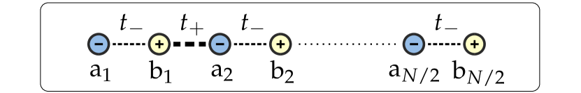
Figure 1: (Colour online) Sketch of the SSH model with $N$ lattice sites subject to the alternating imaginary potential $U$. The minus (plus) sign marks a negative (positive) imaginary potential corresponding to particle sinks (sources).

To evaluate eq. (14) we need to represent this Hamiltonian in the reciprocal space, where the Brillouin zone acts as parameter space. This is done by rewriting the Hamiltonian with creation and annihilation operators in the reciprocal space in the limit $N\to\infty$,

$$H=\sum\limits_{k=-\pi}^{\pi} \begin{pmatrix}c_{\text{a},k}^{\dagger}\,,\,c_{\text{b},k}^{\dagger}\end{pmatrix}$$ (18)

$${\begin{pmatrix}-\mathrm{i}\,\varGamma/2&t_{-}+t_{+}\text{e}^{\,\mathrm{i}k}\\ t_{-}+t_{+}\text{e}^{-\mathrm{i}k}&\mathrm{i}\,\varGamma/2\end{pmatrix}}\begin{pmatrix}\vspace{0.25cm}c_{\text{a},k}^{{\color[rgb]{1,1,1}{\dagger}}}\\ \vspace{0.1cm}c_{\text{b},k}^{{\color[rgb]{1,1,1}{\dagger}}}\end{pmatrix}\leavevmode\nobreak\ ,$$

where the sum runs over discrete values of $k$ in steps of $k=2\pi/N$ and the annihilation operator of an electron with wave number $k$ is given by

$$c_{n}^{{\color[rgb]{1,1,1}{\dagger}}}=\frac{1}{\sqrt{N}}\sum\limits_{k}c_{k}^{{\color[rgb]{1,1,1}{\dagger}}}\text{e}^{-\mathrm{i}\,kr_{n}}$$ (19)

with $r_{n}=an$ and the lattice spacing $a$. The matrix occurring in eq. (18) is the Bloch Hamiltonian $\mathcal{H}(k)$ of the system, which can be decomposed into the Pauli matrices,

$$\mathcal{H}(k) =\big{(}t_{-}+t_{+}\text{cos}(k)\big{)}\sigma_{1}-t_{+}\text{sin}(k)\sigma_{2}-\mathrm{i}\Gamma/2\sigma_{3}$$

$$=\boldsymbol{\mathfrak{n}}(k)\cdot\boldsymbol{\sigma}\;$$ (20)

with a coefficient vector $\boldsymbol{\mathfrak{n}}$ and the Pauli vector $\boldsymbol{\sigma}$. From this form the energy eigenvalues can be obtained explicitly,

$$E_{\pm}(k)=\pm|\boldsymbol{\mathfrak{n}}(k)|\;.$$ (21)

In the limit $\Gamma\rightarrow 0$ the Hamiltonian from eq. (18) reproduces the Hermitian SSH model, which possesses time-reversal, reflection, particle-hole, and a chiral symmetry (represented by $\sigma_{3}$). The introduction of a $\mathcal{PT}$-symmetric non-Hermitian on-site potential $\Gamma$ breaks these symmetries. The non-Hermitian Bloch Hamiltonian is invariant under the combined action of the parity and the time inversion operator. Further the particle-hole symmetry is broken because the sources (sinks) of an electron correspond to sinks (sources) of holes. The non-Hermitian system is therefore symmetric under the action of the combination of the parity and the charge conjugation operator. Further it has no chiral symmetry $\Lambda=\mathfrak{a}_{0}\sigma_{0}+\boldsymbol{\mathfrak{a}}\cdot\boldsymbol{\sigma}$ because a chiral symmetry would fulfil

$$\{\Lambda,\mathcal{H}\} =\sum_{i=0}^{3}\sum_{j=1}^{3}\mathfrak{a}_{i}\mathfrak{n}_{j}\{\sigma_{i},\sigma_{j}\}$$ (22)

$$=2\big{(}\mathfrak{a}_{1}\mathfrak{n}_{1}+\mathfrak{a}_{2}\mathfrak{n}_{2}+\mathfrak{a}_{3}\mathfrak{n}_{3}\big{)}\sigma_{0}+2\mathfrak{a}_{0}\sum_{j=1}^{3}\mathfrak{n}_{j}\sigma_{j}$$

$$\overset{!}{=}0$$

with a coefficient vector $\boldsymbol{\mathfrak{a}}$ which is independent of the value of $k$ , the $2\times 2$ identity matrix $\sigma_{0}$, and the anti-commutation relations $\{\sigma_{i},\sigma_{j}\}=2\delta_{ij}\sigma_{0}$ of the Pauli matrices. Therefore one finds $\mathfrak{a}_{0}=0$, and thus

$$\mathfrak{a}_{1}\mathfrak{n}(k)_{1}+\mathfrak{a}_{2}\mathfrak{n}(k)_{2}+\mathfrak{a}_{3}\mathfrak{n}_{3}\overset{!}{=}0\;,$$ (23)

which cannot be satisfied for a constant vector $\boldsymbol{\mathfrak{a}}$ because the vector $\boldsymbol{\mathfrak{n}}(k)$ rotates on a cylindrical surface as $k$ runs through the Brillouin zone. Hence the non-Hermitian Hamiltonian in eq. (18) does not possess a chiral symmetry. However, this does not mean there is no quantised real part of the Zak phase since its quantisation is ensured by the argument of Hatsugai [43] in the $\mathcal{PT}$-unbroken parameter regime as mentioned above. At the critical point $\Gamma=0$ the system reproduces the Hermitian SSH model, which possesses the previously mentioned symmetries. For $\Gamma<0$ the particle sinks and sources are interchanged leading to a spatially reflected system with the same general properties as the system with $\Gamma>0$.

From the Bloch Hamiltonian (cf. eq. (18)) the complex Zak phase can be calculated following the steps explained in section 3. We choose (c.f. eq. (11a))

$$\begin{split}f_{\Delta\varphi_{n}}(x)\,=\leavevmode\nobreak\ &\Delta\varphi_{n}\,x-2\pi\\ \text{with}\leavevmode\nobreak\ \leavevmode\nobreak\ \leavevmode\nobreak\ x\leavevmode\nobreak\ =\leavevmode\nobreak\ &\frac{k+\pi/a}{2\pi/a}\;,\end{split}$$ (24)

which is the most simple function fulfilling the conditions (11b).

Figure 2 illustrates the gauge smoothing process using the first non-vanishing component $p=1$ of the left basis states as an example. The component $\langle\chi_{1}(\boldsymbol{\alpha}_{j})|_{1}$ of the unnormalised left eigenvector is shown in Figure 2 (a). One can see two different phase branches as a result of the numerical diagonalisation and a constant modulus. After the gauge smoothing and normalisation according to the first step described in section 3 as shown in Figure 2 (b) the modulus varies with the wave number $k$ and there is only one phase branch left, but the basis is not yet single-valued as there is still a phase difference at the boundaries of the Brillouin zone. In this example the factor $X=-1$ has to be used as $\varphi_{1,j}$ jumps from $-\pi$ to $\pi$. After the second step the component $\langle\chi_{1}(\boldsymbol{\alpha}_{j})|_{1}$ of the final left eigenvector is the same at the Brillouin zone boundaries in Figure 2 (c).

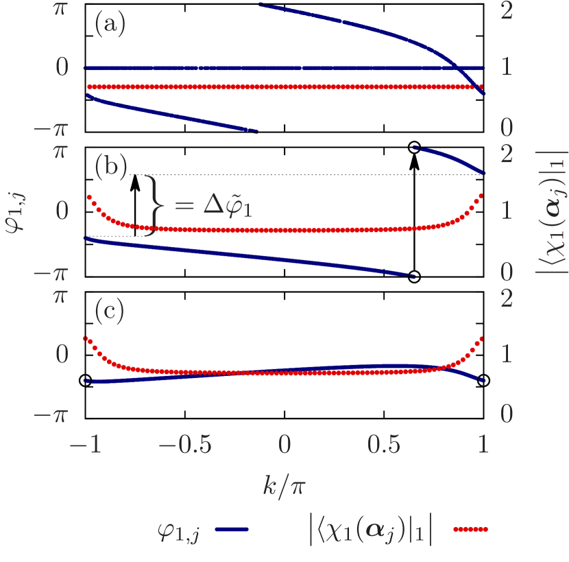
Figure 2: (Colour online) First component of the left handed eigenvector $\langle\chi_{1}(\boldsymbol{\alpha}_{j})|_{1}$ in dependence of the wave number $k$ with $t=1$, $\Delta=1/2$, $\Gamma=1$ and $\theta\approx 0.3\pi$ : (a) Before the steps described in eqs. (6a) and (6b) one can identify two different phase branches (blue line) and a constant modulus (filled red dots). (b) After the steps characterised by eqs. (4a) and (4b) (here $\Delta\tilde{\varphi}_{1}=\varphi_{M,1}-\varphi_{1,1}$ and $X=-1$ c.f. eq. (9)) the phase is smooth within the Brillouin zone but discontinuous at its boundaries, and the modulus varies with $k$. (c) After the gauge smoothing process the phase difference $\Delta\tilde{\varphi}_{1}$ is compensated and the phase is continuous and smooth in the whole Brillouin zone.

The two complex Zak phases $\gamma_{1}$ and $\gamma_{2}$ following from the eigenvector pairs of $\mathcal{H}(k)$ are shown in Figures 3 (a) and (b), where the control parameter $\theta$ is used to describe the difference between the two tunnelling amplitudes $t_{+}$ and $t_{-}$,

$$t_{\pm}=t\,\big{(}1\pm\Delta\text{cos}(\theta)\big{)}$$ (25)

with the mean value of the tunnelling amplitude $t$ and the dimerization strength $\Delta$.

To verify our results we compare them with the analytical ones derived in [37],

$$\gamma_{1/2}=\pi\,\Theta(q-1)\pm\mathrm{i}\frac{\eta}{2}\sqrt{\frac{\nu}{q}}\left(K(\nu)+\frac{q-1}{q+1}\Pi(\mu,\nu)\right)\;,$$ (26)

where $q=t_{+}/t_{-}$ is the ratio of the tunnelling amplitudes, $\eta=\varGamma/(2t_{-})$ and $\nu=4q/((q+1)^{2}-\eta^{2})$ and $\mu=4q/(q+1)^{2}$. $K(\nu)$ and $\Pi(\mu,\nu)$ are elliptic integrals of first and third kind,

$$K(\nu)= \int\limits_{0}^{\pi/2}\frac{\mathrm{d}k}{\sqrt{1-\nu\,\text{sin}^{2}(k)}}\;,$$ (27)

$$\Pi(\mu,\nu)= \int\limits_{0}^{\pi/2}\frac{\mathrm{d}k}{1-\mu\,\text{sin}^{2}(k)\,\sqrt{1-\nu\,\text{sin}^{2}(k)}}\;.$$ (28)

The numerical calculations perfectly reproduce the analytical results. The grey shaded areas in Figure 3 mark the values of $\theta$ for which the system is in a $\mathcal{PT}$-broken phase, for all other values of $\theta$ the system is in a $\mathcal{PT}$-unbroken phase. In the $\mathcal{PT}$-symmetric regime the real part of the complex Zak phase is either $0$ or $\pi$ modulo $2\pi$ and can be used to characterise the topological phase of the system.

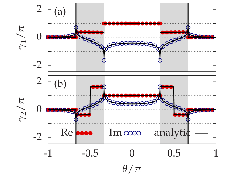
Figure 3: (Colour online) Numerical results of the real part (filled red dots) and the imaginary part (open blue circles) of the complex Zak phases $\gamma_{1}$ (a) and $\gamma_{2}$ (b) following from the Hamiltonian given in eq. (17) in dependence of the control parameter $\theta$ with $t=1$, $\Delta=1/2$ and $\Gamma=1$ (all values in a.u.) compared to the analytical result (real and imaginary part are represented by a solid black line coinciding with the numerical results) following from eq. (26). The grey shaded area marks the $\mathcal{PT}$-broken phase of the Bloch Hamiltonian.

5 Conclusion

We developed a numerical method to determine a gauge-smoothed biorthogonal basis of eigenstates of a $\mathcal{PT}$-symmetric non-Hermitian Hamiltonian required for complex Zak phases. It is also applicable to Hermitian systems. In the course of this we removed the arbitrary and unconnected global phases of the biorthogonal eigenstates of the $\mathcal{PT}$-symmetric Hamiltonian at each point in parameter space and made the basis single-valued. This allows for the calculation of the complex Berry phase by explicitly evaluating eq. (2) even in complicated lattice systems for which no analytical access to the eigenstates is approachable. We demonstrated the action of the gauge smoothing method by applying the developed algorithm to a $\mathcal{PT}$-symmetric extension of the SSH model. An excellent agreement of the numerical and analytical results was found. In future work this provides the basis for the identification of the Zak phase as topological invariant in many-body systems with arbitrary $\mathcal{PT}$-symmetric complex potentials.

References

- [1] V. Mourik, K. Zuo, S. M. Frolov, et al. Signatures of Majorana fermions in hybrid superconductor-semiconductor nanowire devices. Science 336:1003–1007, 2012. doi:10.1126/science.1222360.
- [2] T. D. Stanescu, S. Tewari. Majorana fermions in semiconductor nanowires: fundamentals, modeling, and experiment. J Phys: Condens Matter 25(23):233201, 2013. doi:10.1088/0953-8984/25/23/233201.
- [3] S. R. Elliott, M. Franz. Colloquium: Majorana fermions in nuclear, particle, and solid-state physics. Rev Mod Phys 87:137–163, 2015. doi:10.1103/RevModPhys.87.137.
- [4] A. Stern, N. H. Lindner. Topological quantum computation—from basic concepts to first experiments. Science 339(6124):1179–1184, 2013. doi:10.1126/science.1231473.
- [5] A. Carmele, M. Heyl, C. Kraus, M. Dalmonte. Stretched exponential decay of Majorana edge modes in many-body localized Kitaev chains under dissipation. Phys Rev B 92, 2015. doi:10.1103/PhysRevB.92.195107.
- [6] C.-E. Bardyn, M. A. Baranov, C. V. Kraus, et al. Topology by dissipation. New J Phys 15(8):085001, 2013. doi:10.1088/1367-2630/15/8/085001.
- [7] P. San-Jose, J. Cayao, E. Prada, R. Aguado. Majorana bound states from exceptional points in non-topological superconductors. Sci Rep 6:21427, 2016. doi:10.1038/srep21427.
- [8] C. M. Bender, S. Boettcher. Real spectra in non-Hermitian Hamiltonians having symmetry. Phys Rev Lett 80:5243–5246, 1998. doi:10.1103/PhysRevLett.80.5243.
- [9] M. Znojil. -symmetric square well. Phys Lett A 285(1–2):7, 2001. doi:10.1016/S0375-9601(01)00301-2.
- [10] C. M. Bender, D. C. Brody, H. F. Jones. Complex extension of quantum mechanics. Phys Rev Lett 89:270401, 2002. doi:10.1103/PhysRevLett.89.270401.
- [11] M. Znojil. Decays of degeneracies in -symmetric ring-shaped lattices. Phys Lett A 375(39):3435, 2011. doi:10.1016/j.physleta.2011.08.005.
- [12] H. F. Jones, E. S. Moreira, Jr. Quantum and classical statistical mechanics of a class of non-Hermitian Hamiltonians. J Phys A 43(5):055307, 2010. doi:10.1088/1751-8113/43/5/055307.
- [13] K. Li, P. G. Kevrekidis, B. A. Malomed, U. Günther. Nonlinear -symmetric plaquettes. J Phys A 45(44):444021, 2012. doi:10.1088/1751-8113/45/44/444021.
- [14] H. Mehri-Dehnavi, A. Mostafazadeh, A. Batal. Application of pseudo-Hermitian quantum mechanics to a complex scattering potential with point interactions. J Phys A 43:145301, 2010. doi:10.1088/1751-8113/43/14/145301.
- [15] V. Jakubský, M. Znojil. An explicitly solvable model of the spontaneous -symmetry breaking. Czech J Phys 55:1113, 2005. doi:10.1007/s10582-005-0115-x.
- [16] G. Lévai, M. Znojil. The interplay of supersymmetry and symmetry in quantum mechanics: a case study for the Scarf II potential. J Phys A 35(41):8793, 2002. doi:10.1088/0305-4470/35/41/311.
- [17] N. Abt, H. Cartarius, G. Wunner. Supersymmetric model of a Bose-Einstein condensate in a -symmetric double-delta trap. Int J Theor Phys 54(11):4054–4067, 2015. doi:10.1007/s10773-014-2467-0.
- [18] A. Mostafazadeh. Delta-function potential with a complex coupling. J Phys A 39:13495, 2006. doi:10.1088/0305-4470/39/43/008.
- [19] H. F. Jones. Interface between Hermitian and non-Hermitian Hamiltonians in a model calculation. Phys Rev D 78:065032, 2008. doi:10.1103/physrevd.78.065032.
- [20] E. M. Graefe, H. J. Korsch, A. E. Niederle. Mean-field dynamics of a non-Hermitian Bose-Hubbard dimer. Phys Rev Lett 101:150408, 2008. doi:10.1103/PhysRevLett.101.150408.
- [21] E. M. Graefe, U. Günther, H. J. Korsch, A. E. Niederle. A non-hermitian symmetric Bose-Hubbard model: eigenvalue rings from unfolding higher-order exceptional points. J Phy A 41(25):255206, 2008. doi:10.1088/1751-8113/41/25/255206.
- [22] Z. H. Musslimani, K. G. Makris, R. El-Ganainy, D. N. Christodoulides. Analytical solutions to a class of nonlinear Schrödinger equations with -like potentials. J Phys A 41:244019, 2008. doi:10.1088/1751-8113/41/24/244019.
- [23] W. D. Heiss, H. Cartarius, G. Wunner, J. Main. Spectral singularities in -symmetric Bose-Einstein condensates. J Phys A 46(27):275307, 2013. doi:10.1088/1751-8113/46/27/275307.
- [24] D. Dast, D. Haag, H. Cartarius, G. Wunner. Quantum master equation with balanced gain and loss. Phys Rev A 90:052120, 2014. doi:10.1103/PhysRevA.90.052120.
- [25] R. Gutöhrlein, J. Schnabel, I. Iskandarov, et al. Realizing -symmetric BEC subsystems in closed Hermitian systems. J Phys A 48(33):335302, 2015. doi:10.1088/1751-8113/48/33/335302.
- [26] Y. C. Hu, T. L. Hughes. Absence of topological insulator phases in non-Hermitian -symmetric Hamiltonians. Phys Rev B 84:153101, 2011. doi:10.1103/PhysRevB.84.153101.
- [27] K. Esaki, M. Sato, K. Hasebe, M. Kohmoto. Edge states and topological phases in non-Hermitian systems. Phys Rev B 84:205128, 2011. doi:10.1103/PhysRevB.84.205128.
- [28] C. Yuce. Topological phase in a non-Hermitian symmetric system. Phys Lett A 379(18–19):1213 – 1218, 2015. doi:10.1016/j.physleta.2015.02.011.
- [29] C. Yuce. PT symmetric Floquet topological phase. Eur Phys J D 69(7):184, 2015. doi:10.1140/epjd/e2015-60220-7.
- [30] C. Yuce. Majorana edge modes with gain and loss. Phys Rev A 93:062130, 2016. doi:10.1103/PhysRevA.93.062130.
- [31] M. Klett, H. Cartarius, D. Dast, et al. Relation between -symmetry breaking and topologically nontrivial phases in the Su-Schrieffer-Heeger and Kitaev models. Phys Rev A 95:053626, 2017. doi:10.1103/PhysRevA.95.053626.
- [32] H. Schomerus. Topologically protected midgap states in complex photonic lattices. Opt Lett 38(11):1912–1914, 2013. doi:10.1364/OL.38.001912.
- [33] J. M. Zeuner, M. C. Rechtsman, Y. Plotnik, et al. Observation of a topological transition in the bulk of a non-Hermitian system. Phys Rev Lett 115:040402, 2015. doi:10.1103/PhysRevLett.115.040402.
- [34] X. Wang, T. Liu, Y. Xiong, P. Tong. Spontaneous -symmetry breaking in non-Hermitian Kitaev and extended Kitaev models. Phys Rev A 92:012116, 2015. doi:10.1103/PhysRevA.92.012116.
- [35] S. Weimann, M. Kremer, Y. Plotnik, et al. Topologically protected bound states in photonic parity-time-symmetric crystals. Nat Mater 16(4):433–438, 2017. doi:10.1038/nmat4811.
- [36] J. Zak. Berry’s phase for energy bands in solids. Phys Rev Lett 62:2747–2750, 1989. doi:10.1103/PhysRevLett.62.2747.
- [37] S.-D. Liang, G.-Y. Huang. Topological invariance and global Berry phase in non-Hermitian systems. Phys Rev A 87:012118, 2013. doi:10.1103/PhysRevA.87.012118.
- [38] I. Mandal, S. Tewari. Exceptional point description of one-dimensional chiral topological superconductors/superfluids in BDI class. Physica E 79:180 – 187, 2016. doi:10.1016/j.physe.2015.12.009.
- [39] D. C. Brody. Biorthogonal quantum mechanics. J Phys A 47(3):035305, 2014. doi:10.1088/1751-8113/47/3/035305.
- [40] N. Moiseyev. Non-Hermitian Quantum Mechanics. Cambridge University Press, Cambridge, 2011.
- [41] W. P. Su, J. R. Schrieffer, A. J. Heeger. Solitons in polyacetylene. Phys Rev Lett 42:1698–1701, 1979. doi:10.1103/PhysRevLett.42.1698.
- [42] M. V. Berry. Quantal phase factors accompanying adiabatic changes. Proc R Soc London, Ser A 392(1802):45–57, 1984. doi:10.1098/rspa.1984.0023.
- [43] Y. Hatsugai. Quantized Berry phases as a local order parameter of a quantum liquid. J Phys Soc Jpn 75(12):123601–123601, 2006. doi:10.1143/jpsj.75.123601.
- [44] J. C. Garrison, E. M. Wright. Complex geometrical phases for dissipative systems. Phys Lett A 128(3-4):177–181, 1988. doi:10.1016/0375-9601(88)90905-X.
- [45] B. N. Parlett, D. R. Taylor, Z. A. Liu. A look-ahead Lanczos algorithm for unsymmetric matrices. Math Comp 44(169):105–124, 1985. doi:10.1090/S0025-5718-1985-0771034-2.