Simple models of three coupled $\mathcal{PT}$-symmetric wave guides allowing for third-order exceptional points

Abstract

We study theoretical models of three coupled wave guides with a $\mathcal{PT}$-symmetric distribution of gain and loss. A realistic matrix model is developed in terms of a three-mode expansion. By comparing with a previously postulated matrix model it is shown how parameter ranges with good prospects of finding a third-order exceptional point (EP3) in an experimentally feasible arrangement of semiconductors can be determined. In addition it is demonstrated that continuous distributions of exceptional points, which render the discovery of the EP3 difficult, are not only a feature of extended wave guides but appear also in an idealised model of infinitely thin guides shaped by delta functions.

1 Introduction

It is a well-known fact that the spectra of non-Hermitian quantum systems can exhibit exceptional points of second order (EP2), i.e. branch point singularities at which two eigenstates coalesce [1, 2, 3]. They have been extensively studied theoretically [4, 5, 6, 7, 8, 9, 10, 11, 12, 13, 14, 15, 16, 17] and their physical relevance has been demonstrated in impressive experiments [18, 19, 20, 21, 22, 23, 24, 25, 26].

In much rarer cases exceptional points of higher order (EP$N$) are discussed [27, 28, 29, 30]. In a matrix representation they can be identified by the fact that the matrix is not diagonalisable. With a similarity transformation one can reduce the matrix to a Jordan normal form, where the EP$N$ appears as an $N$-dimensional Jordan block [31]. In a third-order exceptional point (EP3) three states coalesce in a cubic-root branch point singularity, which already turned out to exhibit new effects beyond those of EP2s such as an unusual chiral behaviour [28]. The exchange behaviour of the eigenstates for circles around an EP3 shows a complicated structure. It does not in all cases uncover the typical cubic-root behaviour [29, 32].

Of special interest in the investigation of exceptional points are $\mathcal{PT}$-symmetric systems, i.e. systems whose Hamiltonians are invariant under the combined action of the parity operator $\mathcal{P}$ and the time reversal operator $\mathcal{T}$ [33]. In these systems the exceptional point marks a quantum phase transition, in which real eigenvalues merge under variation of a parameter and become complex if the parameter is varied further in the same direction. The eigenstates of the complex eigenvalues are not $\mathcal{PT}$ symmetric, this is only the case for the eigenstates with real eigenvalues. One speaks of broken $\mathcal{PT}$ symmetry, and the EP marks the position of the $\mathcal{PT}$ symmetry breaking. Since the occurrence of exceptional points is a generic feature of the $\mathcal{PT}$ phase transition a large number of works exists for $\mathcal{PT}$-symmetric quantum mechanics [34, 35, 36, 27, 37, 38, 39, 40, 41, 42, 43, 44, 45, 46, 47, 48, 49], quantum field theories [50, 51], electromagnetic waves [52, 53, 54, 55, 56, 57, 58], and electronic devices [59].

In these papers exceptional points of second order have been investigated in great detail. $\mathcal{PT}$-symmetric optical wave guides, in particular, with an appropriate coupling between them, are ideally suited to generate higher-order exceptional points [29]. Klaiman et al. [60] showed that a detailed theoretical modelling of a setup of two wave guides predicts the occurrence of an EP2, and directly proved it via its signatures, among them an increasing beat length in the power distribution. Exactly this strategy has later been used experimentally [61]. Encouraged by these findings the model was extended by Heiss and Wunner, who added a third wave guide between those with gain and loss to allow for a third-order exceptional point. They studied a simplified model consisting of infinitely thin wave guides modelled by delta functions [30]. In a follow-up paper a detailed investigation of a spatially extended setup with experimentally accessible parameters was used [62]. It was shown that the system is well capable of manifesting a third-order exceptional point in an experimentally feasible procedure.

The purpose of this paper is to show that the essential properties of the system studied in [62] can already be found in much simpler descriptions, allowing for deeper insight. The whole three wave-guide setup can be mapped to a matrix model. In such a matrix model an EP3 can be found in a simple manner. However, the largest benefit is in the predictability of matrix structures allowing for an easy access to an EP3. Since the influence of the physical parameters on the matrix elements is known from the mapping, the matrix can guide the search for appropriate physical parameter ranges.

In [62] it was demonstrated that the EP3 of interest is surrounded by continuous distributions of EP2s or EP3s in the space of the physical parameters. This effect in combination with the fact that an EP3 can show a square-root behaviour for parameter space circles [29, 32] renders its identification difficult. In this paper we show that this difficulty can be studied in the much simpler delta-functions model introduced in [30].

The remainder of the paper is organised as follows. In Section 2 we provide a brief introduction into the system. The matrix model is developed in Section 3, where we introduce the mapping of the full system onto three modes, which can be used to search for the best parameter ranges. In Section 4 we show the appearance of continuously distributed exceptional points in the delta-functions model. The central results are summarised in Section 5.

2 Three optical wave guides with a complex $\mathcal{PT}$-symmetric refractive index profile

The starting point of our investigation is the $\mathcal{PT}$-symmetric optical wave guide system introduced in [62]. It consists of three coupled planar wave guides on a background material of GaAs, which has a refractive index of $n_{0}=3.3$ at the vacuum wavelength used in that study. The refractive index profile is supposed to be $\mathcal{PT}$-symmetric, i.e. it possesses a symmetric real part representing the index guiding profile and an antisymmetric imaginary part describing the gain-loss structure, i.e. $n(x)=n^{*}(-x)$. It extends the idea Klaiman et al. pursued for two wave guides. The physical parameters consist of dimensionless scaling factors $s_{m}$ and $s_{1,2}$ used to define distances in units of a constant length $a=$2.5\text{\,}\mathrm{\SIUnitSymbolMicro m}$$ (cf. Fig. 1)

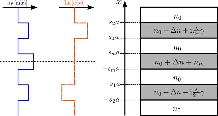
Figure 1: $\mathcal{PT}$-symmetric wave guide setup allowing for the occurrence of an EP3. Three coupled slab wave guides are formed on a background material with refractive index $n_{0}=3.3$ of GaAs via an index variation of $\Delta n=1.3\times 10^{-3}$. The middle wave guide can exhibit an additional index shift given by the value of $n_{m}$. A gain-loss profile is introduced via the imaginary refractive index part $\gamma$. All distances are measured in terms of a constant length scale $a=$2.5\text{\,}\mathrm{\SIUnitSymbolMicro m}$$ via the dimensionless parameters $s_{m}$ and $s_{1,2}$. The variation of the refractive index is only in $x$ direction and obeys $\mathcal{PT}$ symmetry.

and variations of the refractive index. The background index is shifted by a constant value of $\Delta n=1.3\times 10^{-3}$, and an additional shift $n_{m}$ can be applied, to the middle wave guide. The gain-loss parameter is labelled $\gamma$. The vacuum wavelength is assumed to be $\lambda=$1.55\text{\,}\mathrm{\SIUnitSymbolMicro m}$$.

For a wave propagation of transverse electric modes along the $z$ axis the ansatz

$$E_{y}(x,z,t)=\mathcal{E}_{y}(x)\mathrm{e}^{\mathrm{i}(\omega t-\beta z)}$$ (1)

with $k=2\pi/\lambda$ and the propagation constant $\beta$ can be applied, and leads to the wave equation

$$\left(\frac{\partial^{2}}{\partial x^{2}}+k^{2}n(x)^{2}\right)\mathcal{E}_{y}(x)=\beta^{2}\mathcal{E}_{y}(x)\;,$$ (2)

which is formally equivalent to the one-dimensional Schrödinger equation

$$\underbrace{\left(-\frac{1}{2}\frac{\partial^{2}}{\partial x^{2}}+V(x)\right)}_{=H_{\text{sys}}}\psi(x)=E\psi(x)$$ (3)

with the relations

$$V(x) =-\frac{1}{2}k^{2}n(x)^{2}\;,$$ (4a)

$$E =-\frac{1}{2}\beta^{2}\;.$$ (4b)

Thus, the formalism of $\mathcal{PT}$-symmetric quantum mechanics can be used for the setup.

3 Mapping onto a matrix model

In the first approximation we map the full Hamiltonian of the setup shown in Figure 1 to a three-mode matrix model. By this approach we check whether the system can give rise to a third-order branch point in a simple manner. This is clearly the case if the resulting Hamiltonian is of the form proposed in [29], viz.

$$\hat{H}_{\text{math}}=\left(\begin{array}[]{ccc}a-2\mathrm{i}\gamma&\sqrt{2}v&0\\ \sqrt{2}v&0&\sqrt{2}v\\ 0&\sqrt{2}v&b+2\mathrm{i}\gamma\end{array}\right)$$ (8)

with $\gamma,v\in\mathbb{R}$ and $a,b\in\mathbb{C}$. The real and imaginary parts of the diagonal elements simulate the refractive index as well as the gain (loss) behaviour in the wave guides. The parameter $v$ represents a coupling between neighbouring wave guides via evanescent fields, and is thus related to the distance between them. All in all $\hat{H}_{\text{math}}$ reflects a situation in which each wave guide supports a single mode.

However, this matrix is merely an abstract mathematical model without direct connection to an experimental realisation. To establish such connection we use the formal analogy between the wave equation (2) and the one-dimensional Schrödinger equation (3) and calculate a matrix representation of our system in terms of

$$\hat{H}^{\prime}=\langle\psi_{i}|H_{\text{sys}}|\psi_{j}\rangle\;.$$ (9)

For this purpose we assume the same real index difference $\Delta n=1.3\times 10^{-3}$ (and $n_{m}=0$) as well as the same width $w=2a=$5.0\text{\,}\mathrm{\SIUnitSymbolMicro m}$$ for all three wave guides and use the ground state modes of each single potential well with corresponding basis functions $\psi_{i},\psi_{j}$. This results in a matrix of the form

$$\hat{H}^{\prime}=\left(\begin{array}[]{ccc}\alpha+\mathrm{i}\eta&\sigma^{\prime}&\xi\\ \sigma^{\prime}&\alpha&\sigma^{\prime}\\ \xi&\sigma^{\prime}&\alpha-\mathrm{i}\eta\end{array}\right)$$ (13)

with $\alpha,\eta,\xi\in\mathbb{R}$ and $\sigma^{\prime}\in\mathbb{C}$. The use of a common width is compatible only with $s_{m}=1.0$ and $s_{2}-s_{1}=2.0$, which implies that the matrix elements still depend on the doublet $(\gamma,s_{1})$, and thus on the distance $s_{1}-s_{m}$ between the wave guides.

Eq. (13) does not show the form predicted for the appearance of an EP3 from Eq. (8) as $\xi\neq 0$ and $\sigma^{\prime}\in\mathbb{C}$. This corresponds to a situation in which also the two outer wave guides are connected by a coupling of their waves. This can happen due to a too small separation between the wave guides. However, for a sufficiently large separation $s_{1}-s_{m}$ the Hamiltonian $\hat{H}^{\prime}$ reduces to the form

$$\hat{\bar{H}}=\left(\begin{array}[]{ccc}\alpha+\mathrm{i}\eta&\sigma&0\\ \sigma&\alpha&\sigma\\ 0&\sigma&\alpha-\mathrm{i}\eta\end{array}\right)$$ (17)

with $\alpha,\eta,\sigma\in\mathbb{R}$, which resembles the desired form of Eq. (8) for $a=b=0$ up to a constant shift $\alpha$. The transition $\hat{H}^{\prime}\to\hat{\bar{H}}$ can be observed in Figure 2, where the real eigenenergies of Eq. (13) are shown as a function of the wave guides’ distances.

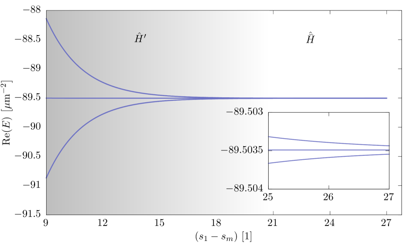
Figure 2: Real eigenenergies $E=-\beta^{2}/2$ of the Hamiltonian $\hat{H}^{\prime}$ as a function of the scaled distance $s_{1}-s_{m}$ between the middle wave guide and the outer ones. As there is a small separation between the wave guides there is comparatively strong coupling among the modes (grey area). With increasing distance the coupling becomes negligible and the system is well described by the new Hamiltonian $\hat{\bar{H}}$ from Eq. (17).

For comparatively small distances the energies are far apart from each other due to a stronger coupling between the modes. In this range only $\hat{H}^{\prime}$ describes the full system correctly. For larger distances the energies approach each other, which means that we likewise obtain an accurate description of the system in terms of the Hamiltonian $\hat{\bar{H}}$. This is the regime, in which a search for an EP3 is most promising.

Knowing the shape of an appropriate wave guide we now focus on a large separation between the wave guides with $s_{m}=1.0$, $s_{1}=28.0$ and $s_{2}=30.0$ and verify the existence of the EP3. We find it in the spectra by varying the gain-loss coefficient $\gamma$. The result is depicted in Figure 3 a).

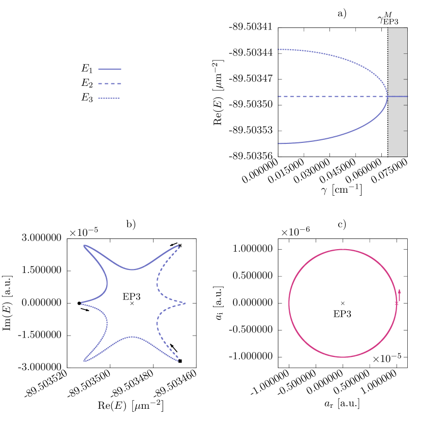
Figure 3: Evidence of a third-order exceptional point in the matrix model for a large separation between the wave guides ($s_{m}=1.0$, $s_{1}=28.0$, $s_{2}=30.0$). The real index difference to the background material ($\Delta n=1.3\times 10^{-3}$) was set to be equal for all three wave guides, i.e. $n_{m}=0$. The coalescence of the three eigenenergies as a function of the non-Hermiticity parameter $\gamma$ is depicted in a) and appears at $\gamma_{\mathrm{EP3}}=0.0636\,\mathrm{cm}^{-1}$. The lower panel shows the characteristic state permutation of an EP3 b) as one performs a closed loop around it in a specific parameter space c). Here we circle the EP3 counter clockwise in the complex plane of the asymmetry parameter $a=a_{\mathrm{r}}+\mathrm{i}a_{\mathrm{i}}$, where the specific symbols mark the starting points of the permutation and the arrows the corresponding direction.

Obviously we obtain the coalescence of all three real eigenenergies for $\gamma_{\mathrm{EP3}}^{M}=0.0636\,\mathrm{cm}^{-1}$ in a cubic root branch point singularity. Beyond this point the spectrum becomes complex with two complex conjugate energies and one with vanishing imaginary part. Note that the middle state stays widely unaffected by an increase of the non-Hermiticity parameter, wich is also found in the more realistic descriptions [30, 62] as well as flat band systems [63, 64].

To ascertain that this is indeed an EP3 we follow a standard procedure and perform a closed loop in a suitable parameter space around the supposed branch point singularity. To do so we have to introduce the complex parameters $a,b$ from Eq. (8) breaking the underlying $\mathcal{PT}$ symmetry. We restrict ourselves to the specific choice $a=b=a_{\mathrm{r}}+\mathrm{i}a_{\mathrm{i}}$ and add this to $\hat{\bar{H}}$, ending up with

$$\hat{H}_{A}=\hat{\bar{H}}+a\left(\begin{array}[]{ccc}1&0&0\\ 0&0&0\\ 0&0&1\end{array}\right)\;.$$ (21)

Using this form the circle is performed in the complex plane of $a$ along an ellipse with the parametrization

$$\left[0,2\pi\right]\to\mathbb{R}^{2}\,,\,\varphi\mapsto\left(\begin{array}[]{c}a_{\mathrm{r}}\\ a_{\mathrm{i}}\end{array}\right)=\left(\begin{array}[]{c}10^{-5}\cos\varphi\\ 10^{-6}\sin\varphi\end{array}\right)$$ (26)

as illustrated in Figure 3 c). The corresponding state permutation is depicted in Figure 3 b) and clearly exhibits the threefold exchange behaviour of an EP3.

4 Continuously distributed exceptional points around the EP3

The third-order exceptional point investigated in Section 3 was verified with a parameter space circle and its typical threefold permutation behaviour. As was found in [62] this can become a difficult task in a realistic setup. On the one hand, not every parameter space circle leads to the threefold permutation. A twofold state exchange misleadingly indicating an EP2 is also possible for certain parameter choices [29, 32]. On the other hand, additional exceptional points, which are accidentally located within the area enclosed by the parameter space loop, can distort the signature of the EP3. In the spatially extended investigation of [62] it turned out that the EP3 is accompanied by continuous distributions of exceptional points in such a way that it is very hard to find a parameter plane, in which a circle reveals the pure cubic-root branch point signature of the EP3. Here we show that this is not only a property of the special shape of the three wave guides used in [62] but a generic feature of three coupled guiding profiles. To do so, we return to the delta-functions model from [30].

The model is given by an effective Schrödinger equation of the form

$$-\psi^{\prime\prime}(x) -\bigl{[}(1+\mathrm{i}\gamma)\delta(x+b)+\Gamma\delta(x)$$

$$\qquad+(1-\mathrm{i}\gamma)\delta(x-b)\bigr{]}\psi(x)=-k^{2}\psi(x)\;,$$ (27)

where three delta-function potential wells are located at $x=\pm b$ and $x=0$. Loss is added to the left well and the same amount of gain is added to the right one via the parameter $\gamma$. The units are chosen in such a way that the strength of the real and imaginary parts of the two outer wells is normalised to unity, while in the middle well we allow for a different depth given by the real parameter $\Gamma>0$, similarly to its spatially extended counterpart from Section 2. As the system is non-Hermitian the eigenvalues $k$ are complex in general with $\mathrm{Re}(k)>0$. We are interested in bound state solutions with real eigenvalues, and the bound state wave functions have the form

$$\psi(x) =\begin{cases}A\mathrm{e}^{kx}&:\;x<-b\\ 2(r\cosh(kx)+\varrho_{1}\sinh(kx))&:\;-b<x<0\\ 2(r\cosh(kx)+\varrho_{2}\sinh(kx))&:\;0<x<b\\ B\mathrm{e}^{-kx}&:\;x>b\end{cases}\;.$$ (28)

As the continuity conditions and the discontinuity conditions for the wave functions and their first derivatives have to be fulfilled at the delta functions we obtain a system of linear equations in the form

$$\mathcal{M}\begin{pmatrix}r\\ \varrho_{1}\\ \varrho_{2}\end{pmatrix} =\mathbf{0}\;,$$ (29)

for which nontrivial solutions exist if the corresponding secular equation

$$\mathrm{det}(\mathcal{M}) =\Gamma\bigl{(}\mathrm{e}^{-4kb}(1+\gamma^{2})-2\mathrm{e}^{-2kb}(\gamma^{2}-2k+1)$$

$$\qquad+\gamma^{2}+(2k-1)^{2}\bigr{)}+2k\bigl{(}\mathrm{e}^{-4kb}(1+\gamma^{2})$$

$$\qquad-\gamma^{2}-(2k-1)^{2}\bigr{)}=0$$ (30)

vanishes. Hence we obtain the eigenvalues $k$ as roots of the determinant $\mathrm{det}[\mathcal{M}](k)\equiv f(k)$ depending on the distance $b$, the non-Hermiticity parameter $\gamma$, and the parameter $\Gamma$ of the middle well. Assuming $k$ to be purely real, the position of the third-order branch point singularity is fixed by

$$f(k)=\frac{\partial f}{\partial k}=\frac{\partial^{2}f}{\partial k^{2}}=0\;.$$ (31)

With $\Gamma_{\mathrm{EP3}}=1.002$ the EP3 appears at

$$\gamma_{\mathrm{EP3}}^{\delta} =0.06527796794065678\;,$$ (32a)

$$b_{\mathrm{EP3}} =6.2012417361076206\;,$$ (32b)

$$k_{\mathrm{EP3}} =0.49584858490334327\;.$$ (32c)

This can be verified by circling this point in the complex plane of the distance $b$ (as it was done in [30]) or by introducing asymmetry parameters breaking the underlying $\mathcal{PT}$ symmetry.

A verification without $\mathcal{PT}$ symmetry breaking, i.e. a circle around the EP3 in the $b$-$\gamma$ space turns out to be impossible in this simplified model as it is always dominated by a signature belonging to an EP2. This suggests the conclusion that in analogy with the spatially extended model from [62] the EP3 may be accompanied by EP2s, which disturb the exchange behaviour. To expose this behaviour we attenuate the condition of Eq. (31) to a twofold zero, from which we get the pair of variables $(k,\gamma)$ or $(k,b)$ and therefore the positions of the EP2s via a two-dimensional root search. The results are shown in Figure 4 (top left). It can be seen that the EP2s are distributed continuously around the EP3 in the $b$-$\gamma$ space.

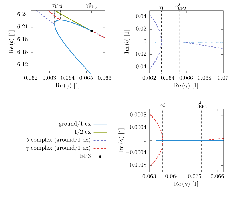
Figure 4: Continuously distributed second-order exceptional points in the $b$-$\gamma$ space of the idealised system made up of three delta-functions potentials. The system’s EP3 appears at $\gamma_{\mathrm{EP3}}^{\delta}$, from which several EP2s arise (top left, solid lines) either between the ground and first excited (1.ex) or between the first and second excited (2.ex) state. They reveal an even more profound branch structure at the points $\gamma_{1}^{c}$ and $\gamma_{2}^{c}$, which can be explained in terms of an analytical continuation of $b$ or $\gamma$ (top right and bottom right).

The lines represent either EP2s between the ground state and the first excited mode or between both excited modes. They coalesce at the position of the EP3 at $\gamma_{\mathrm{EP3}}^{\delta}$ leaving a knee in the parameter space. Moreover there appear more branches at $\gamma_{1,2}^{c}$ along the blue line, which cannot be explained by purely real parameters $b$ and $\gamma$. Hence we either continue $b$ or $\gamma$ analytically into the complex plane and allow for $k\in\mathbb{C}$, which turns the two-dimensional root search into a four-dimensional one. The resulting effects on the $\mathrm{Re}(\gamma)$-$\mathrm{Im}(b)$ space or $\mathrm{Re}(\gamma)$-$\mathrm{Im}(\gamma)$ space are depicted on the right-hand side of Figure 4.

5 Conclusion

In this paper we applied two approximations to the system of three coupled $\mathcal{PT}$-symmetric wave guides studied in [62]. In a mapping of the system to a three-mode matrix model we could show that the matrix can serve as an intuitive guide to parameter regimes, in which the prospects of finding a third-order exceptional point are best. This is exactly the case when the correctly mapped matrix assumes, due to appropriately chosen physical parameters, the shape proposed in [29].

The continuous distributions of EP2s around the EP3 of interest in the space of the accessible physical parameters can be found in the much simpler delta-functions model from [30]. Thus, it is possible to search for adequate physical parameters allowing for the identification of the EP3 via its characteristic threefold state permutation without the need of having to solve the full problem.

In principle the approach of extending the system with additional wave guides to allow for higher-order exceptional points can be continued. With four wave guides it should for example be possible to access a fourth-order exceptional point. The observations made in this work suggest that all further extensions should first be studied in simple approaches before a laborious modelling of a realistic physical setup is done. An $N$-mode matrix model can tell whether a promising search for an EP$N$ in a setup with $N$ wave guides is possible. If this is the case, it can provide rough estimates for suitable physical parameters.

The reduction of the full system to delta functions leads to much simpler equations but preserves the whole richness of effects. As such it can be used as a first access to the structure of the eigenstates. In particular, it can be used to evaluate whether an identification of the EP$N$ via the $N$-fold permutation of the eigenstates seems to be feasible. This can give valuable information before costly numerical calculations of the full system are done.

- [1] T. Kato. Perturbation theory for linear operators. Springer, Berlin, 1966.
- [2] W. D. Heiss. The physics of exceptional points. J Phys A 45(44):444016, 2012. doi:10.1088/1751-8113/45/44/444016.
- [3] N. Moiseyev. Non-Hermitian Quantum Mechanics. Cambridge University Press, Cambridge, 2011.
- [4] W. D. Heiss, A. L. Sannino. Avoided level crossing and exceptional points. J Phys A 23(7):1167, 1990. doi:10.1088/0305-4470/23/7/022.
- [5] W. D. Heiss. Repulsion of resonance states and exceptional points. Phys Rev E 61:929–932, 2000. doi:10.1103/PhysRevE.61.929.
- [6] E. Hernández, A. Jáuregui, A. Mondragán. Non-Hermitian degeneracy of two unbound states. J Phys A 39(32):10087, 2006. doi:10.1088/0305-4470/39/32/S11.
- [7] R. Lefebvre, O. Atabek, M. Šindelka, N. Moiseyev. Resonance coalescence in molecular photodissociation. Phys Rev Lett 103:123003, 2009. doi:10.1103/physrevlett.103.123003.
- [8] H. Cartarius, J. Main, G. Wunner. Exceptional points in the spectra of atoms in external fields. Phys Rev A 79:053408, 2009. doi:10.1103/PhysRevA.79.053408.
- [9] S.-B. Lee, J. Yang, S. Moon, et al. Observation of an exceptional point in a chaotic optical microcavity. Phys Rev Lett 103:134101, 2009. doi:10.1103/PhysRevLett.103.134101.
- [10] S. Longhi. Spectral singularities and Bragg scattering in complex crystals. Phys Rev A 81:022102, 2010. doi:10.1103/PhysRevA.81.022102.
- [11] A. Guo, G. J. Salamo, D. Duchesne, et al. Observation of -symmetry breaking in complex optical potentials. Phys Rev Lett 103:093902, 2009. doi:10.1103/PhysRevLett.103.093902.
- [12] H. Cartarius, N. Moiseyev. Fingerprints of exceptional points in the survival probability of resonances in atomic spectra. Phys Rev A 84:013419, 2011. doi:10.1103/PhysRevA.84.013419.
- [13] R. Gutöhrlein, J. Main, H. Cartarius, G. Wunner. Bifurcations and exceptional points in dipolar Bose-Einstein condensates. J Phys A 46(30):305001, 2013. doi:10.1088/1751-8113/46/30/305001.
- [14] J. Wiersig. Enhancing the sensitivity of frequency and energy splitting detection by using exceptional points: Application to microcavity sensors for single-particle detection. Phys Rev Lett 112:203901, 2014. doi:10.1103/PhysRevLett.112.203901.
- [15] W. D. Heiss, G. Wunner. Resonance scattering at third-order exceptional points. J Phys A 48(34):345203, 2015. doi:10.1088/1751-8113/48/34/345203.
- [16] L. Schwarz, H. Cartarius, G. Wunner, et al. Fano resonances in scattering: an alternative perspective. Eur Phys J D 69(8):196, 2015. doi:10.1140/epjd/e2015-60202-9.
- [17] H. Menke, M. Klett, H. Cartarius, et al. State flip at exceptional points in atomic spectra. Phys Rev A 93:013401, 2016. doi:10.1103/PhysRevA.93.013401.
- [18] M. Philipp, P. v. Brentano, G. Pascovici, A. Richter. Frequency and width crossing of two interacting resonances in a microwave cavity. Phys Rev E 62:1922–1926, 2000. doi:10.1103/PhysRevE.62.1922.
- [19] C. Dembowski, H.-D. Gräf, H. L. Harney, et al. Experimental observation of the topological structure of exceptional points. Phys Rev Lett 86:787–790, 2001. doi:10.1103/PhysRevLett.86.787.
- [20] C. Dembowski, B. Dietz, H.-D. Gräf, et al. Observation of a chiral state in a microwave cavity. Phys Rev Lett 90:034101, 2003. doi:10.1103/PhysRevLett.90.034101.
- [21] B. Dietz, T. Friedrich, J. Metz, et al. Rabi oscillations at exceptional points in microwave billiards. Phys Rev E 75:027201, 2007. doi:10.1103/PhysRevE.75.027201.
- [22] T. Stehmann, W. D. Heiss, F. G. Scholtz. Observation of exceptional points in electronic circuits. J Phys A 37(31):7813, 2004. doi:10.1088/0305-4470/37/31/012.
- [23] M. Lawrence, N. Xu, X. Zhang, et al. Manifestation of symmetry breaking in polarization space with terahertz metasurfaces. Phys Rev Lett 113:093901, 2014. doi:10.1103/PhysRevLett.113.093901.
- [24] T. Gao, E. Estrecho, K. Y. Bliokh, et al. Observation of non-Hermitian degeneracies in a chaotic exciton-polariton billiard. Nature 526(7574):554–558, 2015. doi:10.1038/nature15522.
- [25] J. Doppler, A. A. Mailybaev, J. Böhm, et al. Dynamically encircling an exceptional point for asymmetric mode switching. Nature 537(7618):76–79, 2016. doi:10.1038/nature18605.
- [26] H. Xu, D. Mason, L. Jiang, J. G. E. Harris. Topological energy transfer in an optomechanical system with exceptional points. Nature 537(7618):80–83, 2016. doi:10.1038/nature18604.
- [27] E. M. Graefe, U. Günther, H. J. Korsch, A. E. Niederle. A non-Hermitian symmetric Bose-Hubbard model: eigenvalue rings from unfolding higher-order exceptional points. J Phys A 41(25):255206, 2008. doi:10.1088/1751-8113/41/25/255206.
- [28] W. D. Heiss. Chirality of wavefunctions for three coalescing levels. J Phys A 41(24):244010, 2008. doi:10.1088/1751-8113/41/24/244010.
- [29] G. Demange, E.-M. Graefe. Signatures of three coalescing eigenfunctions. J Phys A 45(2):025303, 2012. doi:10.1088/1751-8113/45/2/025303.
- [30] W. D. Heiss, G. Wunner. A model of three coupled wave guides and third order exceptional points. J Phys A 49(49):495303, 2016. doi:10.1088/1751-8113/49/49/495303.
- [31] U. Günther, I. Rotter, B. F. Samsonov. Projective Hilbert space structures at exceptional points. J Phys A 40(30):8815, 2007. doi:10.1088/1751-8113/40/30/014.
- [32] W. D. Heiss. Some features of exceptional points. In F. Bagarello, R. Passante, C. Trapani (eds.), Non-Hermitian Hamiltonians in Quantum Physics: Selected Contributions from the 15th International Conference on Non-Hermitian Hamiltonians in Quantum Physics, Palermo, Italy, 18-23 May 2015, pp. 281–288. Springer International Publishing, Cham, 2016. doi:10.1007/978-3-319-31356-6_18.
- [33] C. M. Bender, S. Boettcher. Real spectra in non-Hermitian Hamiltonians having symmetry. Phys Rev Lett 80:5243–5246, 1998. doi:10.1103/PhysRevLett.80.5243.
- [34] C. M. Bender, S. Boettcher, P. N. Meisinger. -symmetric quantum mechanics. J Math Phys 40(5):2201, 1999. doi:10.1063/1.532860.
- [35] M. Znojil. Exact solution for morse oscillator in -symmetric quantum mechanics. Phys Lett A 264(2-3):108, 1999. doi:10.1016/S0375-9601(99)00805-1.
- [36] V. Jakubský, M. Znojil. An explicitly solvable model of the spontaneous -symmetry breaking. Czech J Phys 55:1113–1116, 2005. doi:10.1007/s10582-005-0115-x.
- [37] H. F. Jones. Interface between Hermitian and non-Hermitian Hamiltonians in a model calculation. Phys Rev D 78:065032, 2008. doi:10.1103/physrevd.78.065032.
- [38] H. Mehri-Dehnavi, A. Mostafazadeh, A. Batal. Application of pseudo-Hermitian quantum mechanics to a complex scattering potential with point interactions. J Phys A 43:145301, 2010. doi:10.1088/1751-8113/43/14/145301.
- [39] H. F. Jones, E. S. Moreira, Jr. Quantum and classical statistical mechanics of a class of non-Hermitian Hamiltonians. J Phys A 43(5):055307, 2010. doi:10.1088/1751-8113/43/5/055307.
- [40] E.-M. Graefe. Stationary states of a symmetric two-mode Bose-Einstein condensate. J Phys A 45(44):444015, 2012. doi:10.1088/1751-8113/45/44/444015.
- [41] W. D. Heiss, H. Cartarius, G. Wunner, J. Main. Spectral singularities in -symmetric Bose-Einstein condensates. J Phys A 46(27):275307, 2013. doi:10.1088/1751-8113/46/27/275307.
- [42] D. Dast, D. Haag, H. Cartarius, G. Wunner. Quantum master equation with balanced gain and loss. Phys Rev A 90:052120, 2014. doi:10.1103/PhysRevA.90.052120.
- [43] N. Abt, H. Cartarius, G. Wunner. Supersymmetric model of a Bose-Einstein condensate in a -symmetric double-delta trap. Int J Theor Phys 54(11):4054–4067, 2015. doi:10.1007/s10773-014-2467-0.
- [44] R. Gutöhrlein, J. Schnabel, I. Iskandarov, et al. Realizing -symmetric BEC subsystems in closed Hermitian systems. J Phys A 48(33):335302, 2015. doi:10.1088/1751-8113/48/33/335302.
- [45] D. Dast, D. Haag, H. Cartarius, G. Wunner. Purity oscillations in Bose-Einstein condensates with balanced gain and loss. Phys Rev A 93:033617, 2016. doi:10.1103/PhysRevA.93.033617.
- [46] M. Kreibich, J. Main, H. Cartarius, G. Wunner. Realizing -symmetric non-Hermiticity with ultracold atoms and Hermitian multiwell potentials. Phys Rev A 90:033630, 2014. doi:10.1103/PhysRevA.90.033630.
- [47] M. Znojil. Bound states emerging from below the continuum in a solvable -symmetric discrete Schrödinger equation. Phys Rev A 96:012127, 2017. doi:10.1103/PhysRevA.96.012127.
- [48] L. Schwarz, H. Cartarius, Z. H. Musslimani, et al. Vortices in Bose-Einstein condensates with -symmetric gain and loss. Phys Rev A 95:053613, 2017. doi:10.1103/PhysRevA.95.053613.
- [49] M. Klett, H. Cartarius, D. Dast, et al. Relation between -symmetry breaking and topologically nontrivial phases in the Su-Schrieffer-Heeger and Kitaev models. Phys Rev A 95:053626, 2017. doi:10.1103/PhysRevA.95.053626.
- [50] C. M. Bender, V. Branchina, E. Messina. Ordinary versus -symmetric quantum field theory. Phys Rev D 85:085001, 2012. doi:10.1103/PhysRevD.85.085001.
- [51] P. D. Mannheim. Astrophysical evidence for the non-Hermitian but -symmetric Hamiltonian of conformal gravity. Fortschr Phys 61(2-3):140, 2013. doi:10.1002/prop.201200100.
- [52] R. El-Ganainy, K. G. Makris, D. N. Christodoulides, Z. H. Musslimani. Theory of coupled optical -symmetric structures. Opt Lett 32(17):2632–2634, 2007. doi:10.1364/OL.32.002632.
- [53] K. G. Makris, R. El-Ganainy, D. N. Christodoulides, Z. H. Musslimani. Beam dynamics in symmetric optical lattices. Phys Rev Lett 100:103904, 2008. doi:10.1103/PhysRevLett.100.103904.
- [54] A. Mostafazadeh, H. Mehri-Dehnavi. Spectral singularities, biorthonormal systems and a two-parameter family of complex point interactions. J Phys A 42:125303, 2009. doi:10.1088/1751-8113/42/12/125303.
- [55] C. M. Bender, M. Gianfreda, Ş. K. Özdemir, et al. Twofold transition in -symmetric coupled oscillators. Phys Rev A 88:062111, 2013. doi:10.1103/PhysRevA.88.062111.
- [56] S. Bittner, B. Dietz, H. L. Harney, et al. Scattering experiments with microwave billiards at an exceptional point under broken time-reversal invariance. Phys Rev E 89:032909, 2014. doi:10.1103/PhysRevE.89.032909.
- [57] A. Mostafazadeh. Nonlinear spectral singularities of a complex barrier potential and the lasing threshold condition. Phys Rev A 87:063838, 2013. doi:10.1103/PhysRevA.87.063838.
- [58] B. Peng, S. K. Ozdemir, F. Lei, et al. Parity-time-symmetric whispering-gallery microcavities. Nat Phys 10(5):394–398, 2014. doi:10.1038/nphys2927.
- [59] J. Schindler, A. Li, M. C. Zheng, et al. Experimental study of active circuits with symmetries. Phys Rev A 84:040101, 2011. doi:10.1103/PhysRevA.84.040101.
- [60] S. Klaiman, U. Günther, N. Moiseyev. Visualization of branch points in -symmetric waveguides. Phys Rev Lett 101:080402, 2008. doi:10.1103/PhysRevLett.101.080402.
- [61] C. E. Rüter, K. G. Makris, R. El-Ganainy, et al. Observation of parity-time symmetry in optics. Nat Phys 6:192, 2010. doi:10.1038/nphys1515.
- [62] J. Schnabel, H. Cartarius, J. Main, et al. -symmetric waveguide system with evidence of a third-order exceptional point. Phys Rev A 95:053868, 2017. doi:10.1103/PhysRevA.95.053868.
- [63] L. Ge. Parity-time symmetry in a flat-band system. Phys Rev A 92:052103, 2015. doi:10.1103/PhysRevA.92.052103.
- [64] L. Ge, B. Qi. Defect states emerging from a non-Hermitian flat band of photonic zero modes, 2017. arXiv:1704.04713.