Inelastic accretion of inertial particles by a towed sphere

Abstract

The problem of accretion of small particles by a sphere embedded in a mean flow is studied in the case where the particles undergo inelastic collisions with the solid object. The collision efficiency, which gives the flux of particles experiencing at least one bounce on the sphere, is found to depend upon the sphere Reynolds number only through the value of the critical Stokes number below which no collision occurs. In the absence of molecular diffusion, it is demonstrated that multiple bounces do not provide enough energy dissipation for the particles to stick to the surface within a finite time. This excludes the possibility of any kind of inelastic collapse, so that determining an accretion efficiency requires modelling more precisely particle-surface microphysical interactions. A straightforward choice is to assume that the particles stick when their kinetic energy at impact is below a threshold. In this view, numerical simulations are performed in order to describe the statistics of impact velocities at various values of the Reynolds number. Successive bounces are shown to enhance accretion. These results are put together in order to provide a general qualitative picture on how the accretion efficiency depends upon the non dimensional parameters of the problem.

I Introduction

A number of situations involve interactions between small particles suspended in a fluid and a boundary. These include industrial applications, such as sediment deposition in ducts and fouling Henry et al. (2012), but also natural phenomena such as aerosol scavenging by raindrops Pruppacher and Klett (1997) or accretion of dust onto planetary embryos Lissauer (1993). Recent studies have shown that the combined effects of particles inertia and of inelastic shocks among them or with a surface leads to intricate outcomes. For instance, particles can undergo sticky elastic collisions and form clusters under the sole influence of their dissipative viscous drag Bec et al. (2013). Moreover, it was shown that there exists a localization/delocalization transition depending on their Stokes number and their restitution coefficient that rules the long-time inhomogeneities in the particles spatial distribution Belan et al. (2014). This approach, which was initially focusing on random fluid flows vanishing linearly at the boundary, has recently been extended to nonlinear flows mimicking the behavior in viscous boundary layers Belan (2016); Belan et al. (2016). The mechanisms at play are very similar to those ruling the inelastic collapse of randomly forced particles Cornell et al. (1998), but are in that case extended to space-dependent diffusion coefficients. Such a similarity raises two questions. First, one can wonder whether or not a noisy behavior in the particles dynamics is absolutely necessary for observing a collapse to the surface. Thermal-like agitation could indeed be key in activating such a transition, as observed in granular dynamics Cecconi et al. (2003). Conversely a deterministic behavior of the fluid flow close to the boundary, inducing for instance a constant drift that pushes the particles toward the surface, could be an effective way to trigger collapse. A second observation is that inelastic collapse typically occurs in a finite time, so one can conjecture that particles-wall interactions affect not only the stationary long-time distribution but also transient dynamics. This could have noticeable consequences on the question of particle accretion and deposition on a spherical obstacle.

Rain is known to give an important contribution to the transfer of aerosol particles onto the ground. This “wet deposition” originates from the scavenging of particles by drops during their precipitation and is a key ingredient entering cloud-resolving meteorological and climatic models Mircea et al. (2000); Berthet et al. (2010). Aerosols play a central role in atmospheric physics, not only as cloud condensation nuclei but also as hazardous particulate pollutants. Accurate predictions on their lifecycle are thus needed to efficiently estimate both long-term global warming Levy et al. (2013) and pollution washout depending on meteorological conditions Guo et al. (2016). The modeling and parametrization of scavenging is essentially built on the seminal work by Beard Beard (1974) and on the numerical investigation of the collection efficiency of small inertial particles by a sphere in axisymmetric flows Beard and Grover (1974). Such models are still subject to experimental validations Ardon-Dryer et al. (2015); Lemaitre et al. (2017). Accuracy is difficultly achievable because of the variety of physical effects at play including diffusion, electro-scavenging due to particle charges, thermophoresis stemming from the local air cooling by the raindrop, and inertial impaction where sufficiently large aerosols detach from the fluid streamlines to collide with the drop. All these effects fail at providing a satisfactory mechanism for scavenging aerosols with sizes $\simeq 0.1$ to $1\,\mu{\rm m}$. Such ultrafine particles are the most dangerous to health since they are likely to penetrate the respiratory system up to the alveolar region to provoke pulmonary, cardiovascular or brain diseases Chen et al. (2016). Under typical atmospheric conditions, the collection efficiency is dominated by thermal diffusion at small sizes and inertial impaction at larger and attains a minimum well below 1% at intermediate values corresponding to a particle Stokes number (non-dimensional response time) of the order of $0.01$ to $1$.

The presence of a minimum of collection efficiency is above all due to the ineffectiveness of inertial impaction at small particle sizes. Particles with a too weak inertia tend to closely follow the fluid velocity streamlines and are thus swept around the obstacle without impacting it. This effect acts drastically at small values of the Stokes number: There actually exists a critical value below which no particles collide with the sphere Phillips and Kaye (1999). Besides leading to inefficiency in the accretion process, the existence of this cutoff implies that the asymptotics of small Stokes numbers becomes irrelevant, so that analytical results on inertial impaction are particularly arduous. This leaves the sole possibility of employing empirical fitting formula, as for instance proposed by Slinn Slinn (1983), in the models used to address questions where inertial impaction is critical. This is for instance the case in astrophysical situations related to planetesimal growth by dust accretion Sellentin et al. (2013). There, inertial impaction is very important for the early stages of planetesimal growth and might be triggered by the outer gas turbulence of the protoplanetary disk Homann et al. (2016). Most work has nevertheless focused on the collision efficiency of dust with large spherical bodies. It is however known that in the context of dust accretion, the outcome of a collision (coagulation, gravitational capture, bounce, disruption, etc) depends on the details of the impact, such as the kinetic energy, the collision angle and on the material properties of the two bodies Chokshi et al. (1993). Such microphysical features need to be considered in population dynamics models in order to properly predict the timescales of planet growth Windmark et al. (2012); Garaud et al. (2013). Previous work has focused on the probability density of the normal component of impact velocity at the first collision and obtained evidence of a Gaussian distribution whose variance increases as a function of the Stokes number Mitra et al. (2013). However, possible particle bouncing and successive impacts have not yet been considered and could actually lead to a significant depletion of collisional velocities and enhance accretion.

Most previous work has focused on first-impact statistics. Here we consider small inertial particles without molecular diffusion that experience inelastic collisions with a large solid sphere maintained fixed in a mean flow. For that purpose, numerical simulations are performed to investigate several issues related to the particle accretion problem:

1. How does the collision efficiency depend on well-chosen dimensionless numbers (Stokes, Reynolds)?

2. Can particle bouncing and successive inelastic rebounds enhance accretion (inelastic collapse)?

We will see whether or not the actual effect of a deterministic flow at the boundary is different from naive expectations that can be drawn from existing works on inelastic collisions in simple idealized flows.

The paper is organized as follows: the accretion problem (collision efficiency and outcome) is first discussed in Section II together with a succint overview of the model and simulation settings; we evaluate theoretically in Section III whether successive bounces can lead to inelastic collapse within a finite time; the statistics of impact are analyzed numerically in Section IV to characterize the role of successive impacts on accretion while accounting for more realistic particle-sphere interactions.

II The accretion problem and model

We consider the fluid flow past a fixed large sphere. This is a representative case of all the axisymmetric bodies that are likely to accrete small particles in the various situations described in the previous section. The large sphere of diameter $d$ is centered at the origin, and embedded in a flow prescribed to be $\bm{u}=U\bm{e}_{z}$ at infinity and solving the incompressible Navier–Stokes equation with no-slip boundary conditions at the sphere surface. The flow is characterized by the Reynolds number associated with the sphere diameter $Re=U\,d/\nu$, where $\nu$ denotes the kinematic viscosity of the fluid. Numerical simulations are performed using a second-order adaptive finite-element code Hachem et al. (2010). Even if this code gives the possibility to model turbulent flow using a variational multi-scale method, we actually perform direct numerical simulations by prescribing a sufficient resolution to accurately determine all relevant scales.

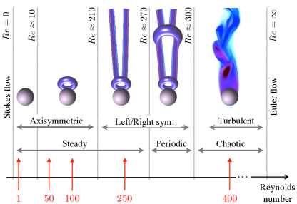
Figure 1: Sketch of the various regimes occurring in the flow past an immobile sphere as a function of the Reynolds number $Re=U\,d/\nu$. The red arrows correspond to the values considered in the numerical simulations of this work.

We have considered different values of the Reynolds number $Re$ which are representative of the various regimes of the flow past a sphere. It is indeed known (see, e.g., Drazin (2002)) that for $Re\lesssim 10$, the fluid velocity is given by Oseen’s flow and thus resembles Stokes’ solution with a tiny fore-and-aft asymmetry. At larger Reynolds a recirculation zone develops downstream. The velocity remains axisymmetric up to $Re\approx 210$ and develops a stationary double-threaded wake above this value. For $Re\gtrsim 270$, vortex shedding starts to occur, the flow becomes time dependent and is characterized by hairpin structures. It then encounters a number of bifurcations and symmetry losses when increasing the Reynolds number Fabre et al. (2008) before becoming chaotic for $Re\gtrsim 300$. All these regimes are sketched in Fig. 1. To span them, we have considered $Re=50$, $100$, $250$ and $400$, and compared them to the ideal cases of a creeping flow ($Re=0$ obtained from the Stokes equation) and an inviscid potential flow (of possible relevance upstream the sphere in the limit $Re\to\infty$). In these two last flows, explicit formulas are used for the fluid velocity field (see, e.g., Falkovich (2011)). Details on the numerical simulation parameters are given in Tab. 1.

Table 1: Parameters of the numerical simulations. All simulations were performed with a sphere of diameter $d=1$, in a domain of size $50\times 50\times 90$ and a fluid velocity maintained at $U=1$ on the upstream and lateral boundaries. The Reynolds number is varied by changing the viscosity $\nu$. The total number of elements $N_{\rm elem}$, the minimum element size $\delta x_{\rm min}$, and the time step, $\delta t$ are varied accordingly.

$Re$	$\nu$	$N_{\rm elem}$	$\delta x_{\rm min}$	$\delta t$
$1$	$1.0$	$3.10^{6}$	$0.005$	$0.002$
$50$	$0.02$	$3.10^{6}$	$0.005$	$0.002$
$100$	$0.01$	$3.10^{6}$	$0.005$	$0.002$
$250$	$0.004$	$3.10^{6}$	$0.005$	$0.002$
$400$	$0.0025$	$6.10^{6}$	$0.002$	$0.001$

These flows past the sphere are seeded with heavy, inertial, point-like particles, whose trajectories $\bm{X}_{\rm p}$ follow

$$\frac{\mathrm{d}^{2}\bm{X}_{\rm p}}{\mathrm{d}t^{2}}=-\frac{1}{\tau_{\rm p}}\left[\frac{\mathrm{d}\bm{X}_{\rm p}}{\mathrm{d}t}-\bm{u}(\bm{X}_{\rm p},t)\right].$$ (1)

The particles are assumed to be much smaller than the smallest active scale of the flow and at the same time sufficiently massive so that added-mass, Magnus, and history effects can be neglected. They only interact with the flow through a viscous drag whose intensity is given by the response time $\tau_{\rm p}=\rho_{\rm p}d_{\rm p}^{2}/(18\,\nu\,\rho_{\rm f})$, where $\rho_{\rm p}$ and $\rho_{\rm f}$ are the particle and fluid mass densities, respectively and $d_{\rm p}$ denotes the diameter of the small particles. In the numerics, the particles are simulated using a Lagrangian approach: their trajectories are tracked by integrating (1) with the fluid velocity at the particle location obtained by linear interpolation from the finite-element field. The particles are uniformly injected far upstream the sphere (at $z=-10\,d$ with a velocity equal to that of the fluid). In the steady axisymmetric settings (Stokes and Euler flows, $Re=1$, $50$ and $100$), the particle dynamics is directly integrated in the plane $(\rho,z)$ where $\rho^{2}=x^{2}+y^{2}$, instead of the full three-dimensional space $(x,y,z)$.

II.1 Collision efficiency

The particles that we consider have some inertia whose intensity is measured by the non-dimensional Stokes number $St=\tau_{\rm p}\,U/d$. When $St\to 0$, they are simple tracers and follow the flow streamlines. Because of the no-penetration condition at the sphere surface, pointwise tracers never collide with it. The particles however deviate from the fluid as soon as $St>0$. For $St\to\infty$, they do not respond anymore to the fluid motion and simply fly ballistically toward the sphere. These opposite behaviors exist independently of the specific boundary conditions, being no-slip as in the case of viscous Stokes flow or free-slip in the case of inviscid Euler (see Fig. 2).

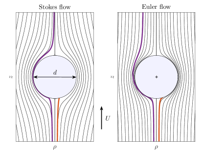
Figure 2: Streamlines corresponding to the two limiting axisymmetric cases of a creeping (Stokes) flow (Left) and a potential inviscid (Euler) flow (Right). Two particle trajectories have been represented in both cases as bold curves. One which collides with the sphere (right-most, in red), and one which does not (left-most, magenta).

The transition from one behavior at $St\ll 1$ to the other at $St\gg 1$ is not progressive but there exists a critical Stokes number $St_{\rm c}$ below which no particles collide with the sphere. $St_{\rm c}$ is a decreasing function of the Reynolds number. It is approximately $0.605$ for $Re=0$ (creeping flow) and approaches asymptotically as $Re\to\infty$ the value $1/24$ obtained in the potential inviscid case Phillips and Kaye (1999). The trajectories represented in Fig. 2 were chosen with Stokes numbers below and above the critical values of these two limiting cases. Note that the reasons why there exists a critical value of the Stokes number differ whether we consider the inviscid potential (Euler) flow or viscous settings. In the former case, the dynamics is linear in the vicinity of the stagnation point on the symmetry axis and $St_{\rm c}$ corresponds to a phase transition where purely real eigenvalues become complex conjugate. For viscous flows, the velocity normal to the sphere surface vanishes quadratically and the problem becomes nonlinear. There always exist colliding trajectories but the Stokes number needs to be large enough for these trajectories to be physically admissible (i.e. recover the fluid velocity at $z=-\infty$). More details can be found in Phillips and Kaye (1999).

For Stokes numbers above the critical value $St_{\rm c}$, there is a beam of particles impacting the sphere around the symmetry axis. In the limit $St\to\infty$, all particles located upstream in the cross section of the sphere will collide with it. For finite values of the Stokes number, some of the particles are deviated by the fluid flow and escape without impacting. The ratio between the fluxes of particles that actually collide and of those contained in the swept volume of the sphere defines $\mathcal{E}_{\rm coll}$, the collision efficiency. $\mathcal{E}_{\rm coll}=1$ for $St\to\infty$, and $\mathcal{E}_{\rm coll}=0$ when $St<St_{\rm c}$.

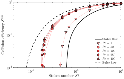
Figure 3: Collision efficiency $\mathcal{E}_{\rm coll}$ as a function of $St$ for the various Reynolds numbers considered here, including $Re=0$ (Stokes creeping flow) and $Re=\infty$ (Euler inviscid flow).

The collision efficiencies measured in our simulations are shown in Fig. 3 as a function of the particles Stokes number. Data corresponding to finite values of the Reynolds number are embraced by those corresponding to the two limiting ideal cases: the Stokes creeping flow ($Re=0$) and the Euler inviscid potential flow ($Re=\infty$). One also observes that for a fixed value of the Stokes number, the efficiency increases as a function of $Re$. This could be only a consequence of the decrease of $St_{\rm c}$ as a function of $Re$. Anyhow, the measured efficiencies remarkably approach the limiting Euler case. When the Reynolds number is large, deviations to the potential flow are restricted to the turbulence that develops in the sphere wake. The probability that a particle collides is essentially determined by the upstream fluid flow which is well described by the potential case with a small viscous boundary layer of thickness $\delta_{\nu}\propto d/\sqrt{Re}$.

Actual values of the collision efficiency are required in the models used for applications. Effective and accurate predictions critically depend upon the values of $\mathcal{E}_{\rm coll}$ that are prescribed. A frequently used fit is that proposed by Slinn in Slinn (1983), namely

$$\left\{\begin{array}[]{l}\mathcal{E}_{\rm coll}\approx\left(\dfrac{St-St_{\rm c}}{St-St_{\rm c}+2/3}\right)^{3/2}\\ \\ St_{\rm c}\approx\dfrac{0.6+(1/24)\log(1+Re/2)}{1+\log(1+Re/2)}.\end{array}\right.$$ (2)

As already stressed in Homann et al. (2016), such a formula predicts $\mathcal{E}_{\rm coll}\propto(St-St_{\rm c})^{3/2}$ when $St\to St_{\rm c}$, which is incompatible with the linear behavior observed in numerics. We provide here an explanation why one expects $\mathcal{E}_{\rm coll}\propto(St-St_{\rm c})$ near the critical Stokes number.

Evaluating the collision efficiency near $St_{\rm c}$ consists in finding whether or not particles initially located at a distance $\rho_{0}\ll d$ from the symmetry axis collide with the sphere. For that, one expands the fluid velocity near the upstream pole of the sphere as

$$u_{z}\approx a\,z^{2}+b\,\rho^{2},\quad u_{\rho}\approx-a\,z\,\rho,$$ (3)

where $a$ and $b$ are positive constants. We have here assumed that the flow is viscous and axi-symmetric around the $\rho=0$ axis. For particles with Stokes number $St=St_{\rm c}(1+\varepsilon)$ where $0<\varepsilon\ll 1$, the particle trajectory $\bm{X}_{\rm p}=(Z,\rho,\theta)$ in cylindrical coordinates reads to leading order for axisymmetric settings

$$\ddot{Z} \approx -(1/\tau^{\rm c}_{\rm p})\left[\dot{Z}-a\,Z^{2}-b\,\rho^{2}-\varepsilon\,\ddot{Z}\right],$$ (4)

$$\ddot{\rho} \approx -(1/\tau^{\rm c}_{\rm p})\left[\dot{\rho}+a\,Z\,\rho\right],$$ (5)

where dots denote time derivatives and $\tau_{\rm p}^{\rm c}$ is the response time corresponding to $St_{\rm c}$. Such a trajectory corresponds to the critical case of a particle touching the sphere at infinite time if the two last terms in the right-hand side of (4) sum to zero. Indeed, in that case $Z$ exactly follows the same dynamics as the critical trajectory located on the symmetry axis for $St=St_{\rm c}$. These two terms cancel out if $\rho^{2}$ is of the order of $\varepsilon$. In addition, as the evolution (5) of $\rho$ is to leading order linear, one obtains that $\rho_{0}^{2}\sim\rho^{2}\sim\varepsilon$, so that $\mathcal{E}_{\rm coll}=(2\rho_{0}/d)^{2}\propto(St/St_{\rm c}-1)$.

The above considerations are limited to the case of viscous flows where, as mentioned earlier, the local dynamics does not change qualitatively at $St=St_{\rm c}$. The situation is different for inviscid potential flows where a transition occurs at $St_{\rm c}$ and some timescales diverge. In that case, the dynamics on the symmetry axis close to the stagnation point reads

$$\ddot{Z}=-(1/\tau_{\rm p})\left[\dot{Z}+c\,Z\right]$$ (6)

with $c$ a positive constant ($c=6\,U/d$ for the Euler flow past a sphere). This linear system has two eigenvalues. They are real for $c\,\tau_{\rm p}\leq 1/4$ and complex conjugate above. They are then equal to

$$\lambda=-({1}/{\tau_{\rm p}})\left[-1\pm i\,\sqrt{4\,c\,\tau_{\rm p}-1}\,\right].$$ (7)

For particle response times right above the critical value, i.e. $\tau_{\rm p}=(1+\varepsilon)/4c$, the frequency associated to the imaginary part of the eigenvalues behave as $\sqrt{\varepsilon}$. Hence particles released at an order unity distance from the sphere need a time of the order of $1/\sqrt{\varepsilon}$ before impacting it. If these particles are at a distance $\rho_{0}$ from the symmetry axis, the transverse distance at impact will be of the order of $\rho=\rho_{0}\exp(C/\sqrt{\varepsilon})$, where $C$ is a positive constant. This exponential growth is due to the fact that the upstream flow is divergent in the $\rho$ direction. The impact occurs only if the particles have not been pushed aside the sphere, that is when $\rho\lesssim d/2$. This implies that the colliding particles must satisfy $\rho_{0}\lesssim(d/2)\exp(-C/\sqrt{\varepsilon})$. Hence, in the case of inviscid flows, the collision efficiency behaves as $\mathcal{E}_{\rm coll}\propto\exp(-C^{\prime}/\sqrt{St-St_{\rm c}})$ above the critical Stokes number and is thus increasing much slower than for viscous flows.

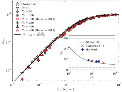
Figure 4: Collision efficiency $\mathcal{E}_{\rm coll}$ as a function of $St/St_{\rm c}-1$ where $St_{\rm c}$ is the critical Stokes number below which no collisions happen. The data of the various simulations are represented as filled symbols, as labeled. The results of Homann et al. Homann et al. (2016) at comparable Reynolds numbers are shown as empty symbols. The solid curve corresponds to the fitting master curve (8). Inset: Critical Stokes number as a function of the Reynolds number for the various runs. The formula (2) proposed by Slinn Slinn (1983) is shown as a solid curve. The two horizontal lines are the two asymptotes (Stokes flow $St_{\rm c}=0.605$ and Euler flow $St_{\rm c}=1/24$).

These phenomenological arguments show that the behavior of the collision efficiency is qualitatively different for viscous and inviscid flows. Thus, for any finite value of the Reynolds number, the dependence of $\mathcal{E}_{\rm coll}$ on the Stokes number will be given by the viscous boundary layer dynamics when $St$ is close to $St_{\rm c}$. The singular behavior of $\mathcal{E}_{\rm coll}$ in inviscid flows can nevertheless have a signature at very large values of $Re$ and lead to a deficit of accretion of particles, even if their Stokes number is well above $St_{\rm c}$. Such an effect could be responsible for overestimating the actual value of $St_{\rm c}$ in experiments. This is not the case in our simulations where we consider moderate values of the Reynolds number. As seen from Fig. 4, a linear boundary-layer behavior of $\mathcal{E}_{\rm coll}$ can clearly be observed for $St-St_{\rm c}\ll 1$. The boundary-layer considerations detailed above also suggests that the collision efficiency depends upon $St/St_{\rm c}$ only. Surprisingly, all data of Fig. 3, including those associated to the Stokes flow, almost collapse on the top of each other once represented as a function of $St/St_{\rm c}-1$ in Fig. 4. An approximation of the master curve is shown as a solid curve. The fitting was obtained from the data corresponding to the Stokes flow and reads

$$\mathcal{E}_{\rm coll}\approx\frac{St-St_{\rm c}}{St+2\,St_{\rm c}}.$$ (8)

Figure 4 also contains data from Homann et al. Homann et al. (2016) which display the same behavior, except at values of the Stokes number which are maybe too close to $St_{\rm c}$. Of course, we have not represented the case of Euler potential flow which displays a very different behavior. We have nevertheless observed that numerical values of $\mathcal{E}_{\rm coll}$ are in that case compatible with $\exp(-C^{\prime}/\sqrt{St-St_{\rm c}})$. The inset of Fig. 4 represents the measured critical Stokes number as a function of $Re$. Again, our data are in good agreement with those of Homann et al. Homann et al. (2016) and seem well fitted by Slinn’s formula (2) for $St_{\rm c}$.

II.2 Particles-boundary interactions

We have discussed in the previous subsection which particles can collide or not with the sphere as a function of their Stokes number and of the flow Reynolds number. This has of course important consequences on accretion. However, the full problem requires qualifying the outcome of collisions, once they occur. Depending whether the particles bounce, break-up, or are absorbed, particle fluxes at the large object boundary surface can be strongly altered. This is illustrated in Fig. 5, which represents the particle concentration for the same flow and particles with the same Stokes number but which are absorbed (Left-hand panel) or inelastically bounce at the surface (Right-hand panel).

Figure 5: Average concentration in the $y=0$ plane of particles with Stokes number $St=\tau_{\rm p}U/d=1$ in a $Re=0$ flow with an absorbing boundary condition at the surface of the sphere (Left) and when they bounce (Right) with a coefficient of restitution $e=0.5$.

We introduce in the following the various possible outcomes of an impact of a small particle with a larger body and how they depend on the particle-boundary interactions. The outcome of a collision depends on a range of parameters and varies with the system considered:

• In the context of meteorology (raindrop formation), binary droplet-droplet interactions in the atmosphere lead to three different collision regimes Ashgriz and Poo (1990); Qian and Law (1997); Saffman and Turner (1956): coalescence, off-center separation and near head-on separation. These various regimes depend mainly on various parameters: the Weber number $We$ (which measures the relative importance of fluid inertia to surface tension), the drop size ratio and the impact parameter (which measures the difference between head-on and grazing collision). It has been observed that coalescence occurs mostly at small $We$ (i.e. when the velocity is small enough not to break droplets) while breakup is significant at higher $We$ especially when the collision is close to the head-on or grazing configurations and often lead to the apparition of satellite droplets.

• In the case of spraying processes in combustion, extra collision regimes have been identified due to the nature of the droplets (chemical composition) Sommerfeld and Kuschel (2016): bouncing can take place at very small $We$ while breakup happens also through stretching or reflexive separation Rabe et al. (2010). These different regimes are similar to those observed in the case of jet breakups Eggers and Villermaux (2008) as well as bubble breakup Clift et al. (1978).

• In the context of wet deposition Pruppacher and Klett (1997); Mircea et al. (2000); Berthet et al. (2010), the scavenging of aerosol particles by falling droplets results in the ’wet deposition’ phenomenon. Studies on the impact between droplets and particles have shown that the capture of aerosol by falling raindrop takes place under various regimes: Brownian and turbulent shear diffusion, inertial impaction, diffusiophoresis, thermophoresis and electrical charge effects. Particle washout thus depends on a number of parameters related to the fluid flow (including the relative humidity) as well as on the nature of the aerosols (chemical composition, size, electromagnetic properties) Chate et al. (2003).

• For collisions between rigid bodies, three regimes have been identified Elimelech et al. (2013); Maximova and Dahl (2006): aggregation (where particles stick to each other to form a larger aggregate), bouncing or fragmentation (where aggregates breakup in several sub-aggregates). The various outcomes depend on several parameters, among which: the impact velocity, the impact angle, the fluid chemical properties (electrolyte concentration, presence of polymers), the particle/aggregate size and geometry.

From this brief overview of the possible outcomes of collisions, three main features can be identified: aggregation (also called capture or coalescence), bouncing and fragmentation (also referred to as breakup). In the present case of small inertial particles impacting a large sphere, we focus mostly on the first two regimes, i.e. capture and bouncing, while the case of fragmentation is left out for future studies. The distinction between capture and bouncing is described by rigid body impact theories Stronge (2004). A collision between two rigid bodies occurs in a very brief period of time during which contact forces prevent particles from overlapping. Such contact forces (or interface pressure) arise in a small area of contact between the two bodies and can result in local deformations. In an elastic collision (typically for hard spheres at small impact velocities), the contact forces at play are conservative (i.e. reversible) such that the energy of the system is conserved. In an inelastic collision, the contact forces dissipate energy (through, e.g., irreversible elasto-plastic deformations). In addition to these forces, a further friction force can arise in the tangential direction if the bodies are rough, leading to sliding motion in the contact area which add further complexity to the system.

To distinguish between elastic and inelastic collisions, we use the notion of the restitution coefficient $e$ which is a macroscopic parameter to characterize the effect of dissipative forces on the energy before and after collisions (a general definition is available in Stronge (2004)). In the following, we assume that surfaces are perfectly smooth (such that friction forces can be neglected) allowing to consider a simplified 1D model for collisions where only the wall-normal component of the particle velocity is modified (there is no energy loss in the tangential direction). More precisely, we define a restitution coefficient as the ratio between the particle wall-normal velocity after collision $v_{\bot}^{+}$ to the wall-normal velocity before collision $v_{\bot}^{-}$:

$$e={v_{\bot}^{+}}/{v_{\bot}^{-}}$$ (9)

The restitution coefficient $e$ ranges between $0$ (inelastic collision) and $1$ (purely elastic collision). It should be noted that the case $e=0$ is actually different from sticky particles since the normal velocity vanishes while the tangential velocity remains unaffected (even for a flat boundary). Considerations of refined restitution coefficients for the outcome of the collision that take into account friction forces (and thus correlations between wall-normal and tangential velocities) are left out of the present paper and will be investigated in future studies.

Following the analysis of collisions between small particles and a sphere made in Section II.1, we consider inelastic collisions where the wall-normal velocity after impact is modified using a single restitution parameter $e$. With these settings one could expect a kind of ’inelastic collapse’ due to a relaxation through multiple rebounds, which could lead to the particle sticking to the surface in a finite time. Upstream of the sphere, the flow is pushing the particle back to the surface after an impact and it bounces again but with a lower energy. Typical trajectories obtained in such a case are illustrated in Fig. 6 for $St=8$ where we can see up to 4 or 5 bounces depending on $e$.

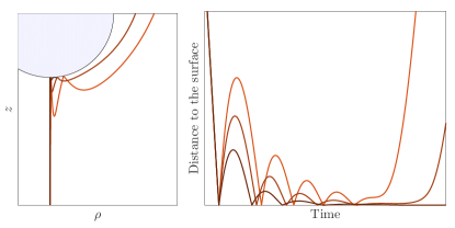
Figure 6: Examples of particle trajectories for $St=10$ and three different restitution coefficients ($e=0.5$, $0.75$ and $1$, dark to light red) in the Stokes flow. The particles are injected at the same initial value of $\rho$ close to the symmetry axis and experience multiple collisions with the sphere. The left panel shows their location in the $(\rho,z)$ plane and the right panel is the distance to the boundary surface as a function of time.

As we will see in the next section such a collapse cannot happen in a finite time in the case of a flow around a sphere, even if $e<1$. Such a collapse can only happen if the particle is trapped due to attractive forces with the large sphere at small scales (such as van der Waals forces, gravitation or electric forces). Considering the simplest case of a Lennard-Jones potential (which is often used to approximate the interaction between a pair of neutral atoms or molecules Israelachvili (2015)), the interaction energy of two molecules separated by a distance $r$ is given by:

$$E_{\rm LJ}(h)=E_{\rm well}\left[\left({r_{m}}/{r}\right)^{12}-2\left({r_{m}}/{r}\right)^{6}\right]$$ (10)

where $E_{\rm well}$ is the depth of the potential well and $r_{m}$ is the distance at which the potential reaches its minimum. The first term on the right hand side is repulsive and corresponds to Pauli repulsion at short ranges (preventing overlap of electron orbitals) while the second term is attractive and describes long-range van der Waals force. The resulting interaction between particles (obtained by integration over the volume of the bodies) is also characterized by a potential well $E_{\rm stick}$ whose value is proportional to the particle radius. After bouncing, a particle can thus escape from the potential well if its kinetic energy after impact is high enough (otherwise, it will remain trapped in the potential well). To evaluate whether such a capture happens, the kinetic energy of the particle after impact is monitored and compared to the potential well $E_{\rm stick}$.

With respect to this analysis, we have chosen to monitor the velocity at impact $v^{\rm coll}$ in order to investigate the range of possible collision outcomes.

III Relaxation through successive collisions

As we have seen in the previous section, particles with a given elasticity can possibly perform multiple successive bounces on the solid boundary. Here, we investigate whether or not the sequence of such collisions can lead to an accretion within a finite time. To simplify the discussion, we suppose that the fluid flow is purely one-dimensional, normal to the solid surface. In the case of the flow around the sphere, this is equivalent to focus on particles located on the symmetry axis. We assume that $\bm{u}=-c\,z^{\alpha}\,\bm{e}_{z}$ with $c>0$ and $\alpha\geq 0$. An attractive force toward the surface corresponds to the case $\alpha=0$, while for Euler flow $\alpha=1$ and for Stokes flow $\alpha=2$.

Let us consider the dynamics between two successive rebounds. We thus suppose that a particle with response time $\tau_{\rm p}$ is initially at the surface $Z_{\rm p}(0)=0$ with a positive velocity $\dot{Z}_{\rm p}(0)=v$. For $\alpha>0$, rescaling time by $s=t/T$ with $T=(v/c)^{1/\alpha}/v$ and introducing $z_{\rm p}(s)=Z_{\rm p}(t)/(v/c)^{1/\alpha}$ leads to

$$\ddot{z}_{\rm p}=-\frac{1}{S_{0}}\left(\dot{z}_{\rm p}+{z}_{\rm p}^{\alpha}\right),\quad{z}_{\rm p}(0)=0\mbox{ and }\dot{z}_{\rm p}(0)=1.$$ (11)

The dynamics depends only on $\alpha$ and the Stokes number $S_{0}=\tau_{\rm p}/T=\tau_{\rm p}\,c^{1/\alpha}\,v^{1-1/\alpha}$. The problem is then to understand under which conditions on $\alpha$ and $St$ the particle touches again the surface $z=0$, and if it does so, at what time and with which velocity.

Let us first consider the case $\alpha=1$. Equation (11) is then linear. One can check that if $S_{0}<1/4$, the particle does not go back to the surface but tends exponentially to it as $t\to\infty$ with a rate $-(1+\sqrt{1-4\,S_{0}})/(2\,S_{0})$. There is another rebound if $S_{0}>1/4$. The solution indeed reads in that case

$${z}_{\rm p}(s)=\frac{1}{\omega}{\rm e}^{-s/(2\,S_{0})}\sin(\omega\,s),\mbox{ with }\omega=\frac{\sqrt{4\,S_{0}-1}}{2\,S_{0}}.$$ (12)

The rebound is at time $\Delta s=\pi/\omega$ and the impact velocity is $\dot{z}_{\rm p}(\Delta s)=-\exp(-\pi/\sqrt{4\,S_{0}-1})$.

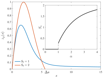
Figure 7: Two trajectories of the system (11) with $\alpha=2$ associated to values of the Stokes number $S_{0}$ below (in blue) and above (in red) the critical Stokes number $S_{\star}(\alpha\!=\!2)\approx 1.18$. Inset: critical Stokes number $S_{\star}$ as a function of the fluid velocity exponent $\alpha$.

For $\alpha\neq 1$ the system is nonlinear and cannot be easily integrated analytically. Nevertheless, when $\alpha>1$, there still exists a critical Stokes number $S_{\star}(\alpha)$ such that the particles touches again the surface only if $S_{0}>S_{\star}$. This is illustrated in Fig. 7 in the case $\alpha=2$. When $S_{0}<S_{\star}$, the trajectory approaches zero only asymptotically as a power law ${z}_{\rm p}\propto s^{-1/(\alpha-1)}$. The critical Stokes number is represented as a function of $\alpha$ in the inset of Fig. 7. As can be seen from the left-hand side of Fig. 8, $S_{0}=S_{\star}$ corresponds to the case when the critical trajectory (red bold curve) starts from the initial value $z_{\rm p}=0$ and $\dot{z}_{\rm p}=1$. When $\alpha<1$, all trajectories hit the surface in a finite time with a finite velocity, as can be seen from the phase portrait on the right-hand side of Fig. 8.

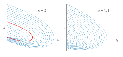
Figure 8: Phase portraits of the $(z_{\rm p},\dot{z}_{\rm p})$ dynamics for $\alpha=2$ (left) and $\alpha=1/2$ (right). When $\alpha>1$ and for any value of the Stokes number $S_{0}$, there exists a critical trajectory (represented as a bold red line) such that all trajectories above touch $z_{\rm p}=0$ in a finite time with a finite velocity and all those below are tending asymptotically to the origin. When $\alpha<1$, there is no such critical trajectory and all initial conditions lead to touch $z_{\rm p}=0$ in a finite time.

Hence, all configurations lead to bounce again on the surface if $S_{0}$ is sufficiently large. The dynamics can be further reduced when $S_{0}\gg 1$. To leading order the linear damping term in (11) can indeed be disregarded and $\ddot{z}_{\rm p}\approx-z_{\rm p}^{\alpha}/S_{0}$ with $z_{\rm p}(0)=0$ and $\dot{z}_{\rm p}(0)=1$. Then, rescaling both time and space by $S_{0}^{1/(\alpha+1)}$, one gets rid of the dependence on $S_{0}$. This implies that when $S_{0}\gg 1$, the time to next collision scales as $\Delta s\propto S_{0}^{1/(\alpha+1)}$. In this approach, we have neglected the time-irreversibility of the particle dynamics. Consequently, the impact velocity is to first order $\dot{z}_{\rm p}(\Delta s)\approx-1$. Next order corrections are obtained by looking at the kinetic energy budget

$$\frac{1}{2}\dot{z}^{2}_{\rm p}(\Delta s)-\frac{1}{2}\dot{z}^{2}_{\rm p}(0)=-\frac{1}{S_{0}}\int_{0}^{\Delta s}\left[\dot{z}^{2}_{\rm p}+\dot{z}_{\rm p}\,z_{\rm p}^{\alpha}\right]\mathrm{d}s.$$ (13)

The second term in the integral, which corresponds to the work done by the fluid velocity, is to leading order time symmetric and thus integrates to zero. The main contribution to the energy dissipation is thus coming from the first term and corresponds to the viscous damping along the time-reversible trajectory. As $\dot{z}_{\rm p}=O(1)$, the energy loss between two rebounds is then of the order of $\Delta s/S_{0}\sim S_{0}^{-\alpha/(\alpha+1)}$.

We now turn to reinterpreting these results in terms of successive rebounds experienced by a given particle. Let us assume that the particle undergoes a sequence of bounces on the solid surface at times $t_{n}$ where $n$ indexes the $n$-th collision. At $t=t_{n}^{+}$, the particle leaves the surface with a velocity denoted $v_{n}$. As seen above, the dynamics up to time $t_{n+1}=t_{n}+\Delta t_{n}$ depends solely on $\alpha$ and on the Stokes number $S_{n}=\tau_{\rm p}\,c^{1/\alpha}\,v_{n}^{1-1/\alpha}$. As the particle looses kinetic energy at each bounce, we expect $v_{n}$ to be decreasing sequentially. This implies that $S_{n}$ increases as a function of $n$ if $\alpha<1$ and decreases if $\alpha>1$. In this latter case, we have also seen above that there exists a critical Stokes number below which the particle does not touch again the surface within a finite time. Consequently any collision sequence is finite when $\alpha>1$. Any particle that is thrown toward the surface is experiencing a finite number of collisions until it has dissipated enough energy. It then converges only asymptotically (as a power law with exponent $-1/(\alpha-1)$) towards $z=0$ and there is no accretion within a finite time. The dynamics between two bounces roughly consists of two stages: The first one is characterized by a dissipation of the particle kinetic energy when it goes away from the solid boundary; The second step consists then in an entrainment of the particle by the fluid flow toward the surface. When $\alpha>1$, the fluid velocity decreases too fast when $z\to 0$ and the first step prevails. Notice that the effect of non-elastic collisions (i.e. a restitution coefficient $e<1$) increases dissipation and thus accentuates this phenomenon.

The situation is different when $0<\alpha<1$. The Stokes number $S_{n}$ increases as a function of $n$, so that dissipation becomes less and less important. Any particle that is thrown toward the surface bounces and experiences an infinite sequence of collisions. After sufficiently many rebounds, $S_{n}$ is large enough to apply the asymptotic results discussed above. The time between the $n$-th and $(n+1)$-th collisions reads $\Delta t_{n}\sim T\,\Delta s\sim v_{n}^{(1-\alpha)/(1+\alpha)}$. The sequence of impact velocities satisfies

$$v_{n+1} = -e\,v_{n}\,\dot{z}_{\rm p}(\Delta s)\simeq e\,v_{n}\,\left(1-C\,S_{n}^{-\frac{\alpha}{1+\alpha}}\right)$$

$$\simeq e\,v_{n}\,\left(1-C\,\tau_{\rm p}^{-\frac{\alpha}{1+\alpha}}c^{-\frac{1}{1+\alpha}}v_{n}^{\frac{1-\alpha}{1+\alpha}}\right),$$

where $e$ is the restitution coefficient of the particles on the surface and $C$ is a positive constant. This recurrence relation gives for $n$ large

$$v_{n}\sim\left\{\begin{array}[]{ll}n^{-\frac{1+\alpha}{1-\alpha}}&\mbox{ for }e=1,\\ e^{n}&\mbox{ for }e<1.\end{array}\right.$$ (14)

For $e=1$, this behavior implies that $\Delta t_{n}\sim 1/n$ and thus $t_{n}$ diverges. The collision sequence lasts forever and an infinite time is required for the particle to stick to the surface. Conversely, if $e<1$, the inter-collision time $\Delta t_{n}$ tends exponentially to zero and its series converges to a finite time $t_{\star}$ at which the particle is accreted at the surface. This closes the case $0<\alpha<1$, the two extreme values needing to be treated separately.

For $\alpha=0$, which corresponds to a constant attractive force between the particle and the solid surface, one cannot proceed in terms of $S_{n}$ as above but the system can be explicitly integrated, leading for $n$ large to $\Delta t_{n}\simeq 2\tau_{\rm p}v_{n}/c$ and $v_{n+1}\simeq e\,v_{n}(1-4v_{n}/(3c))$. One thus obtains exactly the same long-term behavior as for $0<\alpha<1$.

The case $\alpha=1$ corresponds to a free slip boundary condition for the fluid velocity at the solid surface. As we have seen previously, the Stokes number reads $S_{n}=c\,\tau_{\rm p}=S_{0}$ and is then independent of $v_{n}$. If $S_{0}>1/4$, the time between successive collisions is constant $\Delta t_{n}=\pi/(c\,\omega)$, where $\omega(S_{0})$ is given in (12). We thus have $t_{n}\propto n$. The kinetic energy is linearly damped between successive collisions and thus converges exponentially to $0$ as

$$v_{n}\propto\exp\left[n\left(\log e-{\pi}/{\sqrt{4S_{0}-1}}\right)\right].$$ (15)

The effect of inelasticity is just to accelerate the exponential decrease. The particle converges exponentially fast to the boundary and there is no accretion within a finite time.

To end this section, let us shortly summarize our findings. A surprising result is that the only instance when there is accretion in a finite time by successive bounces requires two conditions to be satisfied: the collisions should be inelastic ($e<1$) and the fluid velocity should scales as $u(z)\propto-z^{\alpha}$ with $\alpha<1$. In the cases of physical relevance to the accretion by a sphere, we have $\alpha\geq 1$ and the particles are only approaching asymptotically the surface, exponentially fast for $\alpha=1$ and as a power law for $\alpha>1$. Hence, the mechanism leading to particle accretion cannot be related to any kind of inelastic collapse. It is thus needed to introduce other criterions to determine whether or not particles are sticking to the solid surface. As motivated in Sec. II.2, a relevant quantity is the kinetic energy upon impact (or equivalently the modulus of the impact velocity) whose statistics are clearly given by the sequence $v_{n}$ and discussed in next section for the problem of the flow past a sphere.

IV Impact statistics

We now turn to describing impact velocities statistics obtained from the numerical simulations of the flow past a sphere at the various values of the Reynolds number mentioned in Sec. II. We have seen in the previous section that particles cannot approach the sphere with a vanishing velocity within a finite time through an inelastic collapse. Thus, the possibility that some particles stick to the sphere is necessarily related to the introduction of a finite critical impact velocity below which accretion occurs (see Sec. II.2). This motivates studying the statistics of the modulus $v^{\rm coll}=|\mathrm{d}\bm{X}_{\rm p}/\mathrm{d}t|$ of the particles velocity at impact as well as its average value $v=\langle v^{\rm coll}\rangle$. The idea is to understand how inelastic rebounds influence the distribution of $v$. As we have seen in previous section, particles can indeed undergo successive collisions and the impact velocity $v_{n}$ at the $n$-th bounce can be possibly related to that at the previous collision. For that reason, we start with the statistics of the velocity $v^{\rm coll}_{1}$ at the first collision.

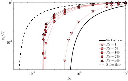
Figure 9: Average of the modulus of the impact velocity $v_{1}=\langle v_{1}^{\rm coll}\rangle$ at the first collision, as a function of the Stokes number for the various Reynolds numbers, including the limiting cases of the Stokes creeping flow and the inviscid potential flow.

Figure 9 shows the average $v_{1}=\langle v_{1}^{\rm coll}\rangle$ $v_{1}^{\rm coll}$ of the velocity modulus at first impact over all particles that collide at least once with the sphere. Again, as for the collision efficiencies, all data are contained in between the two limiting cases of the Stokes and Euler flows. Despite the fact that the Reynolds numbers span different regimes of the flow past a sphere, there is no evidence of any abrupt change in the average impact velocity. Colliding particles are indeed only influenced by the upstream flow, which actually does not undergo any discontinuous changes when $Re$ increases. In addition, the curves are ordered: For a fixed Stokes number, the average impact velocity grows as a function of the Reynolds number and becomes closer to the potential flow. This can be explained by the fact that the viscous boundary layer becomes thinner when $Re$ increases, and this is the place where particles are the most efficiently slowed down. The convergence to the inviscid case is faster at larger Stokes numbers. In that limit, the effect of the boundary layer is indeed becoming weaker because the time during which it affects particles dynamics becomes less than their response time. Note that there is a wide gap in impact velocity amplitude when moving from Stokes to Euler flow. This important increase is due to the fact that the tangential component of the velocity does not vanish in the inviscid case.

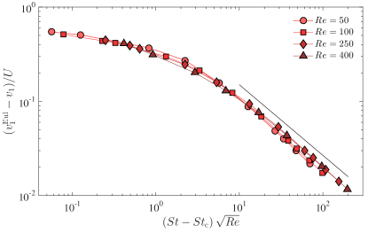
Figure 10: Deviations from the inviscid potential case of the average impact velocity at the first collision. They collapse on the top of each other when represented as a function of $(St-St_{c})\,\sqrt{Re}$. The black line shows a slope $-3/4$.

Figure 10 represents the deviation from the Euler inviscid case of the average impact velocity as a function of the Stokes number. We indeed observe that the deviations vanish when the Stokes number increases. This can be understood with the following argument. Let us suppose that a particle is entering the viscous boundary layer, i.e. is at a distance $\delta_{\nu}\propto d/\sqrt{Re}$ from the surface, with a radial velocity $v_{1}^{\rm Eul}$ that is resulting from the action of the inviscid Euler flow. For a sufficiently large Reynolds number, we assume that the fluid velocity seen by the particle is indeed that of the Euler potential flow until it reaches a distance $\delta_{\nu}$ from the sphere. For large Stokes numbers, the fluid velocity in the boundary layer is always much smaller that the particle velocity. The particle is thus decelerated as if it was in a fluid at rest and impacts the surface with a velocity $v_{1}\simeq v_{1}^{\rm Eul}-\delta_{\nu}/\tau_{\rm p}$. The deviation to the Euler flow is thus indeed decreasing with the Stokes number. This phenomenology also suggests that the deviations are just a function of $St\sqrt{Re}=U\tau_{\rm p}/\delta_{\nu}$. Such a scaling is indeed confirmed in Fig. 9 where representing the average impact velocity as a function of $(St-St_{\rm c})\sqrt{Re}$ allows one to collapse the results associated to the various Reynolds numbers. Surprisingly, such a scaling seems to reasonably extend to the moderate values of the Stokes and/or Reynolds numbers ($Re=1$ has a similar trend as the one for Stokes flow and is thus not shown). At large values, the deviations to the Euler case decreases approximatively as $v_{1}^{\rm Eul}-v_{1}\sim(St\sqrt{Re})^{-3/4}$. Such a behavior, which is different from that obtained above with one-dimensional phenomenological arguments, is certainly due to the spherical geometry of the boundary layer.

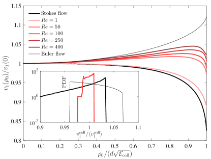
Figure 11: $v_{1}^{\rm coll}$ at the first collision as a function of the injection location $\rho_{0}$ for $St=2$ and the various Reynolds number that we have considered. Inset: Probability density function of the first impact velocity $v_{1}^{\rm coll}$ for $St=2$ and various flows (Stokes flow, $Re=100$, and Euler flow).

The behavior of the average impact velocity seems rather simple, at least for the first collision, and displays qualitative features that resemble much those of the collision efficiency. This could lead to postulate that the more likely the collisions are, the more energetic they are. However, the actual outcomes of collisions cannot be inferred from such an average: They depend on whether or not the individual collision energies of each particle are above or below a critical value. This leads to studying how the impact velocity varies among the colliding particles. Figure 11 shows the average value of $v_{1}(\rho_{0})=\langle v_{1}^{\rm coll}\,|\,\rho_{0}\rangle$ conditioned on the initial distance $\rho_{0}$ of the particle from the symmetry axis. It is here represented for $St=2$ and the various values of the Reynolds number that we have considered. One observes that the two limiting cases of Stokes creeping flow and Euler potential flow display very different qualitative behaviors. In Stokes flow $v_{1}(\rho_{0})$ attains its maximum on the symmetry axis and decreases with $\rho_{0}$ while in Euler flow the potential flow attains a minimum at $\rho_{0}=0$ and then increases. These two different behaviors are related to the very different nature of the near-surface dynamics. In particular, the impact velocity vanishes at $\rho_{0}=(d/2)\,\sqrt{\mathcal{E}_{\rm coll}}$ in the Stokes case. This value corresponds to the colliding particles that are the furthest from the axis of symmetry. As we have seen in Sec. II.1, this corresponds to the initial conditions of the critical trajectory that delimits colliding from non-colliding particles in a quadratic viscous boundary layer (see, e.g., the red bold trajectory on Fig. 8). Such a trajectory is actually touching the sphere surface but only after an infinite time and with a vanishing velocity. Such a trajectory does not exist in the potential flow which vanishes linearly at the sphere surface, as long as $St>St_{\rm c}=1/24$. In this case the impact kinetic energy is essentially given by the amount of deceleration experienced by the particles before touching. The structure of Euler’s potential flow is such that the $z$ component of the fluid velocity at a distance of the order of $d/2$ from the symmetric axis is higher than $U$. Thus the most eccentric particles are those which are the less slowed down, explaining the increase of $v_{1}(\rho_{0})$ as a function of $\rho_{0}$. Finite values of the Reynolds number yield an intermediate behavior: The impact velocity first increases when moving away from the symmetry axis, as in the potential case, and vanishes for $\rho_{0}=(d/2)\,\sqrt{\mathcal{E}_{\rm coll}}$, under the effect of the viscous boundary layer. It attains a maximum in between these two extremes.

The conditional average $v_{1}(\rho_{0})$ leads to an expression for the distribution of the impact velocities if we assume that the particles are homogeneously distributed far upstream. We can indeed write

$$p(v_{1})=p(\rho_{0})\,\left|\frac{\mathrm{d}\rho_{0}}{\mathrm{d}v_{1}}\right|=\frac{1}{\mathcal{E}_{\rm coll}\,(d/2)^{2}}\,\left|\frac{\mathrm{d}\rho_{0}^{2}}{\mathrm{d}v_{1}}\right|.$$ (16)

The corresponding distributions are shown in the inset of Fig. 11. One recovers the two qualitatively different cases of the creeping and potential flows. The distribution in Euler flow is rather flat and bends down at the largest values of $v_{1}$. Conversely the Stokes flow leads to a peaked distribution associated to the flat behavior of $v_{1}$ close to $\rho_{0}=0$. For intermediate Reynolds numbers, the distribution is obtained as a superposition of these two behaviors. The peak persists at the maximal value of $v_{1}$, which is now attained at a finite $\rho_{0}$ rather than on the symmetry axis. Also, the distribution contains two steps associated to the two branches of $v_{1}\mapsto\rho_{0}$.

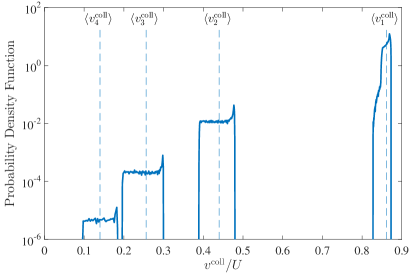
Figure 12: Probability density function of the impact velocity $v^{\rm coll}$ for $Re=100$, $St=2$ and $e=1$. The distribution is multimodal, with the various modes associated to successive bounces of the particles. The vertical dashed lines show the averages impact velocities $\langle v_{n}^{\rm coll}\rangle$ at the $n$-th collision.

Now that we have described impact velocity statistics at the first collision, we extend here this approach to the case of bouncing particles. Figure 12 shows the probability density function of the impact velocity $v^{\rm coll}$ for particles with $St=2$, a coefficient of restitution $e=1$ in the $Re=100$ flow. One clearly observes a multimodal distribution. The right-most bump corresponds to the first impact and has a shape as given above when considering the conditional average of $v_{1}^{\rm coll}$. The other modes to the left are associated to the successive rebounds of the particles. Their shapes are similar to each other but do not exactly reproduce the first-collision distribution. All modes are characterized by a flat region at small values associated to a quadratic minimum on the symmetry axis, and a peak at large values due to the maximum of impact velocity. When successive bounces occur, two phenomena are at play in order to predict the shape of the next mode in the distribution of $v^{\rm coll}$. The first is a decrease of the typical value of $v^{\rm coll}$, which might be described by the results of previous section. The second relates to the fact that only a fraction of bouncing particles will touch again the sphere at a later time. This diminishes the probability weight of each mode when $v^{\rm coll}$ decreases. The combination of these two effects results in an enlargement of each mode when the number of bounces increases. In some cases other than the one shown in Fig. 12, different modes can even superpose. Except that, all results associated to other values of $St$, $e$ and $Re$ display similar behaviors. To complete the picture, we have represented in Fig. 13 the average impact velocity $\langle v^{\rm coll}_{n}\rangle$ at the $n$-th impact. When the Reynolds number is large enough, two behaviors are visible as a function of $n$: $\langle v^{\rm coll}_{n}\rangle$ starts with decreasing exponentially during the first collisions. This corresponds to bounces with a large enough energy such that the particles exit again the viscous boundary layer and the dynamics is close to that given in Eq. (15). Once the collisions are not sufficiently energetic, the particles are trapped in the viscous boundary layer and the impact velocity decreases faster than an exponential.

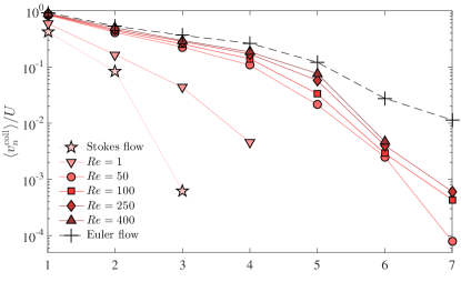
Figure 13: Average of the impact velocity $\langle v^{\rm coll}_{n}\rangle$ at the $n$-th bounce as a function of $n$ for $St=2$, $e=1$ and the various Reynolds number that we have considered.

To complete the picture, we finally propose a way to interpret previous results in terms of an accretion efficiency. For that purpose, we focus on the case of the Stokes creeping flow which, as long as near-boundary dynamics are concerned, is qualitatively representative of flows developing a viscous layer and is easily amenable for a detailed systematic study. As explained in Sec. II.2, we consider here the simplest model for accretion: A particle sticks to the sphere as soon as its impact kinetic energy is less than a threshold which behaves linearly as a function of the small particle size. The relevant parameter is thus $\gamma=\min_{n}v_{n}^{\rm coll}/(U\,St^{1/4})$, where the minimum is over all experienced collisions. For given settings (type of particles and of fluid, nature of the sphere surface) accretion occurs when $\gamma$ is less than a fixed dimensionless critical value $\gamma_{\star}$.

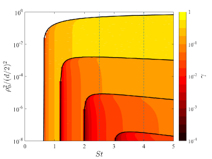
Figure 14: Minimal value of the impact parameter $\gamma=\min_{n}v_{n}^{\rm coll}/(U\,St^{1/4})$ (colored background and level lines) as a function of the particles Stokes number $St$ and of the square $\rho_{0}^{2}$ of their initial distance to the symmetry axis in the Stokes creeping flow and for a restitution coefficient $e=1$. The two vertical lines correspond to the cut shown in Fig. 15.

Figure 14 shows in the case of purely elastic particles ($e=1$) how the impact parameter $\gamma$ depends upon both the particles Stokes number and their initial distance $\rho_{0}$ from the symmetry axis. We have represented here the minimal value of $\gamma$ that a particle experiences when it has multiple bounces, such as a part of the graph that is below a fixed value $\gamma_{\star}$ defines particles which are actually sticking to the sphere. The white area in the left/top of the figure corresponds to values of $\rho_{0}$ and $St$ for which no collision occur and $\gamma$ is not defined. This area is delimited by the collision efficiency, that is by the curve $\rho_{0}^{2}/(d/2)^{2}=\mathcal{E}_{\rm coll}(St)$. Below it, in the colored area, at least one collision occurs. This area is itself divided into several islands (here four) associated to successive rebounds of the particles. Each of these islands is bounded from above and the left by a critical curve which defines the set of parameters for which particles are indeed experiencing at least $n$ collisions. The behavior of these curves as $\rho_{0}\to 0$ defines a critical value of the Stokes number $St_{\rm c}^{(n)}$ below which no particle experiences $n$ collision. Of course, $St_{\rm c}^{(1)}$ is given by the critical Stokes number $St_{\rm c}$ discussed in Sec. II.1. The typical values of $\gamma$ are decreasing from one island to that below, because of the dissipation occuring between successive bounces. In each island, $\gamma$ is minimal close to the upper/left boundary curve. This is because particles with such settings are exactly falling on a critical trajectory: They approach asymptotically the sphere and thus touch at an infinite time with a vanishing velocity. For the data shown in Fig. 14, the impact parameter $\gamma$ decreases when $St$ increases. We however expect that at much larger values of $St$, the impact velocity stabilizes to $v^{\rm coll}\simeq U$, so that the impact parameter should decrease as $\gamma\simeq St^{-1/4}$.

Figure 15: Impact parameter $\gamma$ for the Stokes flow and elastic particles ($e=1$) for two values of the Stokes number ($St=1.5$ and $St=4$). The horizontal dashed line correspond to a specific choice $\gamma_{\star}=0.1$ of the accretion critical parameter. All particles such that $\gamma<\gamma_{\star}$ stick to the sphere. The inset represents for the same settings the accretion efficiency associated to this specific value of $\gamma_{\star}$, as a function of the Stokes number.

To get a better grasp on the interpretation of Fig. 14 in terms of accretion efficiency, we have represented in Fig. 15 two cuts for $St=2.5$ and $St=4$ of the impact parameter $\gamma$ as a function of $\rho_{0}^{2}$. The rebounds islands now appear as steps. Assume that we fix the value $\gamma_{\star}$ of the critical impact parameter. The accreting particles are those which were located at an initial distance $\rho_{0}$ from the symmetric axis satisfying $\gamma(\rho)<\gamma_{\star}$. The accretion efficiency is then obtained by integrating the infinitesimal flux $\propto\rho_{0}\,\mathrm{d}\rho_{0}\propto\mathrm{d}\rho_{0}^{2}$ associated to these values. As an illustration, we consider $\gamma_{\star}=0.1$ (horizontal dashed line in Fig. 15). For $St=4$, all particles colliding three times or more stick to the sphere. In addition, a small fraction of the particles colliding once or twice will stick when they are close to the critical trajectories. This contribution corresponds to the steep dips separating successive plateaux. In the case $St=2.5$, again all particles colliding at least three times will accrete, together with those corresponding to the neighborhood of critical trajectories. However an additional fraction of the particles colliding only twice will stick to the sphere. Putting together all these contribution leads to an evaluation of the accretion rate, that is of the ratio between the particles actually sticking to the sphere and those included upstream in the sphere cross-section. This efficiency is shown as an inset in Fig. 15, again for Stokes’ flow, $e=1$, and the specific choice $\gamma_{\star}=0.1$. The resulting curve has a non-trivial dependence upon $St$ resulting from the various possible behaviors described above.

Notice that we have here chosen to represent data for the elastic case $e=1$. Lesser values of the restitution leads to qualitatively equivalent results with of course a stronger depletion of impact velocities from one bounce to the next but simultaneously, lesser particles experiencing such a rebound. Because of this competition, inelasticity can either enhance or reduce adhesion and its effect is non monotonic. The dependence upon $e$ of the number of collisions that can be experienced by given particles is illustrated in Fig. 16 for Stokes’ creeping flow. The black lines separating the various colored areas are given by the value of the $n$-collisions critical Stokes numbers $St_{\rm c}^{(n)}$. One indeed observes that for a given value of the Stokes number, the maximal number of successive rebounds decreases as a function of $e$.

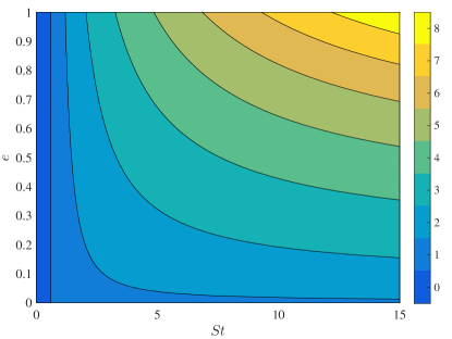
Figure 16: Maximum number of collisions experienced by particles in the Stokes flow, as a function of the Stokes number $St$ and of the restitution coefficient $e$. The black lines show the dependence upon $e$ of the critical Stokes number $St_{c}^{(n)}$ above which particles experience at least $n$ bounces.

V Concluding remarks

We have here focused on the accretion of small particles by a large fixed sphere embedded in a mean flow and we have investigated the effect of inelastic collisions with the sphere. We have characterized the collision efficiency as a function of the two dimensionless parameters (Reynolds and Stokes numbers). In particular, there is a critical Stokes number below which no collision occurs and we have observed that the collision efficiency depends on the Reynolds number based on the sphere diameter only through the value of this critical Stokes number. Besides, our theoretical analysis has demonstrated that successive inelastic collisions do not lead to any kind of inelastic collapse since multiple bounces do not provide enough energy dissipation for the particles to stick to the surface within a finite time. Yet, adding a refined criteria which accounts for particle-surface microphysical interactions can change significantly these results. Here, we have chosen to assume that the particles can stick if their kinetic energy at impact is below a certain threshold. Numerical simulations have shown that successive bounces can possibly enhance accretion regardless of the Reynolds number.

The present numerical simulations also provide interesting qualitative results. It has indeed been shown that, in the case of a Stokes flow, the accretion efficiency has a non-trivial behavior as a function of the Stokes number for a given value of the critical impact parameter ($\gamma_{\star}$ below which particles stick to the surface). In fact, it appears that there is a ’selective’ (or preferential) accretion of specific particle sizes: The accretion efficiency is relatively high at low Stokes number but drops significantly for a narrow range of particle Stokes numbers (around $St=1$). In the context of wet deposition, such a selective accretion can prove to be dramatic in the scavenging of ultrafine particles (within the micrometer range) which are the most dangerous to health. For that reason, it will be also interesting to investigate how the accretion efficiency evolves as a function of the particle Stokes number for other flows (Euler flow, turbulent flows at various Reynolds number) and to verify whether such a selective accretion remains valid in such cases.

These results raise additional questions on the accretion of small particles by a large sphere, among which:

1. What is the effect of diffusion? It has indeed been shown that multiple bounces cannot provide any kind of inelastic collapse in the absence of molecular diffusion. In principle, adding diffusion will give two effects: On the one hand it will alter the results at small values of the Stokes number since the existence of a critical Stokes number disappears. On the other hand, diffusion will grant inelastic collapse for sufficiently small values of the restitution coefficient.

2. What is the effect of more realistic particle-sphere interactions? The present simulations have been performed in the simple case of a flow past a sphere without accounting for specific particle-surface interactions such as: electro-magnetic forces or gravitation (in the context of astrophysical flows), surface tension or capillary forces (in the context of bubble/droplet growth). Besides, more realistic outcomes of collisions can also be investigated by taking into account friction forces and their effect on particle rotation.

3. What is the effect of geometry? A large part of the present results, even at a qualitative level, have been obtained in the case of a flow past a sphere. In that case, it has been seen that bouncing particles can escape downstream if their tangential velocity after impact is high enough to prevent them from coming back to the sphere surface. This situation is specific to the case of a flow past a sphere but can be significantly different in the case of a different geometry such as a flat infinite boundary. This will be the topic of future studies. In particular, we aim at analyzing the effect of successive bounces on the inelastic collapse in the case of particles impacting a flat boundary, such as a channel flow.

References

- Henry et al. (2012) C. Henry, J.-P. Minier, and G. Lefèvre, Adv. Colloid Interface Sci. 185, 34 (2012).
- Pruppacher and Klett (1997) H. Pruppacher and J. Klett, Microphysics of Clouds and Precipitation (Kluwer Academic, Dordrecht, 1997).
- Lissauer (1993) J. J. Lissauer, Annu. Rev. Astron. Astrophys. 31, 129 (1993).
- Bec et al. (2013) J. Bec, S. Musacchio, and S. S. Ray, Phys. Rev. E 87, 063013 (2013).
- Belan et al. (2014) S. Belan, I. Fouxon, and G. Falkovich, Phys. Rev. Lett. 112, 234502 (2014).
- Belan (2016) S. Belan, Physica A 443, 128 (2016).
- Belan et al. (2016) S. Belan, A. Chernykh, V. Lebedev, and G. Falkovich, Phys. Rev. E 93, 052206 (2016).
- Cornell et al. (1998) S. J. Cornell, M. R. Swift, and A. J. Bray, Phys. Rev. Lett. 81, 1142 (1998).
- Cecconi et al. (2003) F. Cecconi, A. Puglisi, U. M. B. Marconi, and A. Vulpiani, Phys. Rev. Lett. 90, 064301 (2003).
- Mircea et al. (2000) M. Mircea, S. Stefan, and S. Fuzzi, Atmos. Environ. 34, 5169 (2000).
- Berthet et al. (2010) S. Berthet, M. Leriche, J.-P. Pinty, J. Cuesta, and G. Pigeon, Atmos. Res. 96, 325 (2010).
- Levy et al. (2013) H. Levy, L. W. Horowitz, M. D. Schwarzkopf, Y. Ming, J.-C. Golaz, V. Naik, and V. Ramaswamy, J. Geophys. Res. 118, 4521 (2013).
- Guo et al. (2016) L.-C. Guo, Y. Zhang, H. Lin, W. Zeng, T. Liu, J. Xiao, S. Rutherford, J. You, and W. Ma, Environ. Pollut. 215, 195 (2016).
- Beard (1974) K. Beard, J. Atmos. Sci. 31, 1595 (1974).
- Beard and Grover (1974) K. Beard and S. Grover, J. Atmos. Sci. 31, 543 (1974).
- Ardon-Dryer et al. (2015) K. Ardon-Dryer, Y.-W. Huang, and D. J. Cziczo, Atmos. Chem. Phys. 15, 9159 (2015).
- Lemaitre et al. (2017) P. Lemaitre, A. Querel, M. Monier, T. Menard, E. Porcheron, and A. I. Flossmann, Atmos. Chem. Phys. 17 (2017).
- Chen et al. (2016) R. Chen, B. Hu, Y. Liu, J. Xu, G. Yang, D. Xu, and C. Chen, Biochim. Biophys. Acta 1860, 2844 (2016).
- Phillips and Kaye (1999) C. Phillips and S. Kaye, J. Aerosol Sci. 30, 709 (1999).
- Slinn (1983) W. Slinn, Atmospheric Sciences and Power Production Chap.11 (1983).
- Sellentin et al. (2013) E. Sellentin, J. Ramsey, F. Windmark, and C. Dullemond, Astron. Astrophys. 560, A96 (2013).
- Homann et al. (2016) H. Homann, T. Guillot, J. Bec, C. Ormel, S. Ida, and P. Tanga, Astron. Astrophys. 589, A129 (2016).
- Chokshi et al. (1993) A. Chokshi, A. Tielens, and D. Hollenbach, Astrophys. J. 407, 806 (1993).
- Windmark et al. (2012) F. Windmark, T. Birnstiel, C. Ormel, and C. P. Dullemond, Astron. Astrophys. 544, L16 (2012).
- Garaud et al. (2013) P. Garaud, F. Meru, M. Galvagni, and C. Olczak, Astrophys. J. 764, 146 (2013).
- Mitra et al. (2013) D. Mitra, J. S. Wettlaufer, and A. Brandenburg, Astrophys. J. 773, 120 (2013).
- Hachem et al. (2010) E. Hachem, B. Rivaux, T. Kloczko, H. Digonnet, and T. Coupez, J. Comput. Phys. 229, 8643 (2010).
- Drazin (2002) P. Drazin, Introduction to Hydrodynamic Stability (Cambridge University Press, Cambridge, 2002).
- Fabre et al. (2008) D. Fabre, F. Auguste, and J. Magnaudet, Phys. Fluids 20, 051702 (2008).
- Falkovich (2011) G. Falkovich, Fluid mechanics: A short course for physicists (Cambridge University Press, Cambridge, 2011).
- Ashgriz and Poo (1990) N. Ashgriz and J. Poo, J. Fluid Mech. 221, 183 (1990).
- Qian and Law (1997) J. Qian and C. Law, J. Fluid Mech. 331, 59 (1997).
- Saffman and Turner (1956) P. Saffman and J. Turner, J. Fluid Mech. 1, 16 (1956).
- Sommerfeld and Kuschel (2016) M. Sommerfeld and M. Kuschel, Exp. Fluids 57, 187 (2016).
- Rabe et al. (2010) C. Rabe, J. Malet, and F. Feuillebois, Phys. Fluids 22, 047101 (2010).
- Eggers and Villermaux (2008) J. Eggers and E. Villermaux, Rep. Prog. Phys. 71, 036601 (2008).
- Clift et al. (1978) R. Clift, J. R. Grace, and M. E. Weber, Bubbles, drops, and particles (Academic Press, New York, 1978).
- Chate et al. (2003) D. Chate, P. Rao, M. Naik, G. Momin, P. Safai, and K. Ali, Atmos. Environ. 37, 2477 (2003).
- Elimelech et al. (2013) M. Elimelech, J. Gregory, and X. Jia, Particle deposition and aggregation: measurement, modelling and simulation (Butterworth-Heinemann, Oxford, 2013).
- Maximova and Dahl (2006) N. Maximova and O. Dahl, Current opinion in colloid & interface science 11, 246 (2006).
- Stronge (2004) W. J. Stronge, Impact mechanics (Cambridge University Press, Cambridge, 2004).
- Israelachvili (2015) J. N. Israelachvili, Intermolecular and surface forces (Academic Press, Amsterdam, 2015).