Acoustic resonance in periodically sheared glass

Abstract

Using molecular dynamics simulation, we study acoustic resonance in low-temperature glass by applying a small periodic shear at a boundary wall. Shear wave resonance occurs as the frequency $\omega$ approaches $\omega_{\ell}=\pi c_{\perp}\ell/L$ ($\ell=1,2,3,...)$. Here, $c_{\perp}$ is the transverse sound speed and $L$ is the cell length. At resonance, large-amplitude sound waves appear after many cycles even for very small applied strains. They then induce plastic events, which are heterogeneous in space and intermittent on time scales longer than the oscillation period $2\pi/\omega$. From these irreversible particle motions, there arises strong dissipation suppressing the growth of sounds. After many resonant cycles, we observe a phenomenon of forced aging, where the shear modulus (measured after switching off the oscillation) is increased significantly. Sometimes, exceptionally large plastic events and system-size sliding motions induce a transition from resonant to off-resonant states. At resonance, translational diffusion becomes appreciable as well as aging due to enhanced configurational changes.

Introduction.– Systems with oscillating degrees of freedom can resonate to an externally applied periodic perturbation as its frequency $\omega$ approaches a resonance one $\omega_{r}$ Landau ; Mook ; Nature . In fact, parametric resonance has been observed in various systems with spin waves Suhl and surface waves Faraday . It is well known that small-amplitude mechanical perturbations can greatly excite particular sound modes in many systems (including musical instruments). Such acoustic resonance has been used to accurately determine the elastic moduli RUS , when the resonance width $\Delta\omega$ is sufficiently small in the frequency range. In crystals, dislocation motions give rise to damping of large-amplitude sounds, so $\Delta\omega$ should depend on the defect density damp . For fluids, we should include the transport coefficients and the nonlinear terms in the hydrodynamic equations to describe resonance of longitudinal sounds. In particular, in fluids near gas-liquid criticality, resonance saturation is due to the singular bulk viscosity Moldover .

In this Letter, we report unique aspects of acoustic resonance in glass at low temperature $T$. Here, we should mention recent papers on dynamics of glass under periodic shear in the low frequency limit Pine ; Keim ; Priez ; Hern ; Regev ; Sood ; Sastry ; Berthier ; Schall ; Haya . These papers have confirmed that the particles motions can be microscopically reversible for small strain amplitude $\gamma_{0}$ but become partially irreversible with increasing $\gamma_{0}$ at low $T$. In contrast, as $\omega\to\omega_{r}$ with small $\gamma_{0}$, the energy input from a wall accumulates in the cell even if it is small in one cycle. Thus, after many cycles, there appear regions with relatively large strains, where plastic events occur heterogeneously and intermittently on time scales longer than the period $t_{p}=2\pi/\omega$ Yamamoto ; Anael . Inducing random particle motions and emission of sounds Shiba , they give rise to a dissipation mechanism, which suppresses the growth of sounds and determines $\Delta\omega$.

Between two parallel walls with distance $L$, the reflection time of shear waves is $t_{r}=2L/c_{\perp}$, where $c_{\perp}$ is the transverse sound speed. If one wall is oscillated at a small $\gamma_{0}$, shear wave resonance occurs for $t_{r}=\ell t_{p}$ or for $\omega=\pi\ell c_{\perp}/L$ ($\ell=1,2,\cdots)$, where the wave nodes are at the walls. However, this criterion is only approximate because of the following. First, the sound modes in glass are highly heterogeneous and the continuum theory holds only at very long wavelengths Gelin ; Sch ; Elliott ; Monaco ; Barrat ; Reichman ; KawaJCP . Second, the amplified sound waves at resonance are largely deformed from sinusoidal forms, where plastic events are proliferated and the linear elasticity does not hold.

In amplified sounds in glass, the particles should noticeably jump out of cages. We shall indeed detect enhanced diffusion at resonance. Moreover, if the system is at resonance for a long time, there should be acceleration of the aging processes (which are extremely slow in quiescent states) Nagel ; Lacks . In fact, we shall find a significant increase in the shear modulus $G$ after many resonant cycles. This effect may be called resonance hardening.

Simulation method.– Our system is a two-dimensional binary mixture in glassy states. In a $L\times L$ cell, the particle numbers are $N_{1}=N_{2}=N/2$ with $N=4000$. The particle pairs separated by $r$ interact via potentials,

$$\phi_{\alpha\beta}(r)=\epsilon({\sigma_{\alpha\beta}}/{r})^{12}-C_{\alpha\beta}\quad(r<r_{\rm c}),$$ (1)

where we introduce $\epsilon$, $\sigma_{1}$, and $\sigma_{2}=1.4\sigma_{1}$ with ${\sigma_{\alpha\beta}}=({\sigma_{\alpha}}+{\sigma_{\beta}})/2$. Here, $\phi_{\alpha\beta}=0$ for $r\geq r_{\rm c}=4.5\sigma_{\alpha\beta}$ with the constant $C_{\alpha\beta}$ ensuring the continuity of $\phi_{\alpha\beta}$ at $r=r_{\rm c}$. The mass ratio is $m_{1}/m_{2}=1.96$. We will measure space, time, and temperature in units of $\sigma_{1}$, $t_{0}=\sigma_{1}(m_{2}/\epsilon)^{1/2}$, and $\epsilon/k_{B}$, respectively. Then, the cell length is $L=70.2$.

To the cell ($0<y<L$), we attached two boundary layers in the regions $-L/16<y<0$ and $L<y<17L/16$. Each layer contains 250 particles bound to pinning points ${\mbox{\boldmath$R$}}_{j}$ on it by the spring potential $\phi_{j}=100\epsilon|{\mbox{\boldmath$r$}}-{\mbox{\boldmath$R$}}_{j}|^{2}/\sigma_{1}^{2}$, where ${\mbox{\boldmath$R$}}_{j}$ were determined in a liquid state Shiba . These boundary particles interact with those in the cell via the potentials in Eq.(1), so layer motions along the $x$ axis induce shear motions in the cell. Keeping the lower layer at rest, we moved the upper one along the $x$ axis as

$$u_{x}(L,t)=-d\sin(\omega t)\quad(t>0),$$ (2)

where $d$ is a small displacement. In this Letter, the mean applied strain $\gamma_{0}=d/L$ is very small (0.002 for $d=0.15$).

To prepare initial glassy states, we started with a liquid at a high $T$, lowered $T$ to $0.01$ below the glass transition, and waited for a time of $10^{3}$, where we used Nosé-Hoover thermostats in the three space regions. After these steps, we removed the thermostat in the cell at $t=0$, keeping those in the boundary layers. Using this initial state for each $d$ and $\omega$, we applied the shear in Eq.(2); then, the local temperature (the local average of the kinetic energy per particle) became inhomogeneous due to heating, but it was fixed at $0.01$ in the boundary layers.

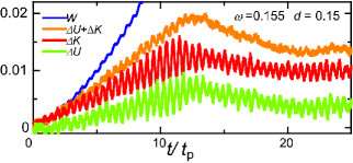
Figure 1: (Color online) Evolution after application of periodic shear with $d=0.15$ at first resonance frequency $\omega=\omega_{1}=0.155$. Here, $0<t<25t_{p}$ with $t_{p}=40.5$. Plotted are deviations of kinetic energy $K$, potential energy $U$, and sum $K+U$ from their initial values divided by $N\epsilon$. $W(t)$ (in blue) is energy input from the upper boundary layer in units of $N\epsilon$.

Resonance.– In this Letter, the resonant frequencies are close to $\omega_{\ell}=\pi\ell c_{\perp}/L$ up to $\ell=3$. The latter are the frequencies of the standing shear waves. In our initial state, we have $c_{\perp}=(G/\rho)^{1/2}=3.5$, where $G=16~{}\epsilon/\sigma_{1}^{2}$ is the shear modulus and $\rho=1.20~{}{m}_{2}/\sigma_{1}^{2}$ is the mass density. In Supplementary Material (SM) Supp , we present microscopic analysis of the vibrational modes Gelin ; Sch ; Elliott ; Monaco ; Barrat ; Reichman , where the first one with the lowest frequency represents the shear wave with $\ell=1$ and the quasi-localized ones have higher frequencies for our system size. In SM Supp , we also provide a movie of resonant growth.

At the first resonance $\omega=\omega_{1}=0.155$ with $d=0.15$, Fig. 1 displays growth of the kinetic energy $K(t)$, the potential energy $U(t)$, and their sum $H(t)$ of the particles in the cell. The deviations $\Delta K(t)=K(t)-K(0)$ and $\Delta U(t)=U(t)-U(0)$ from the initial values consist of oscillating parts due to sounds and slowly evolving parts due to heating. The sum of the former is the total acoustic energy with weaker oscillation, which grows up to $0.005N\epsilon$ for $d=0.15$ and $0.02N\epsilon$ for $d=0.3$. The temperature in the middle is higher than 0.01 by $0.025$ for $d=0.15$ and by $0.04$ for $d=0.3$ for $t/t_{p}\gtrsim 20$. We also plot the energy input from the upper layer to the cell, denoted by $W(t)$ (see its definition in Ref. input ). It is initially changed into the acoustic energy but is eventually balanced with the energy transport from the cell to the boundary layers Shiba .

We next examine how the resonance occurs as $\omega$ is varied. We define the average displacement length by

$${\Delta r}(\omega,\tau)=\sum_{0\leq n-n_{0}<M}\sum_{i}\frac{|{\mbox{\boldmath$r$}}_{i}(nt_{p}+\tau)-{\mbox{\boldmath$r$}}_{i}(nt_{p})|}{MN},$$ (3)

where $0<\tau\leq t_{p}$. We sum over the particles in the cell and over $M$ consecutive cycles ($n_{0}\leq n<n_{0}+M)$. With $n_{0}=50$ and $M=200$, Fig. 2 gives ${\Delta r}(\omega,\tau)$ vs $\omega$ for (a) $\tau=t_{p}/4$ and (b) $\tau=t_{p}$. The displacements in (a) consist of reversible (periodic) and irreversible (non periodic) ones, while those in (b) are all irreversible. Amplification occurs around $\omega\sim 0.15,0.33$, and $0.53$, which correspond to $\omega_{\ell}$ ($\ell=1,2,3$). For $\omega\sim 0.15$, the reversible ones are dominant such that ${\Delta r}$ in (a) is much larger than ${\Delta r}$ in (b). For $\omega\sim 0.33$ and 0.53, the resonance width $\Delta\omega$ is large with enhanced irreversibility. In Fig. 3, we display typical amplified displacements in a quarter period ($n<t/t_{p}<n+1/4$), where $\omega=0.155$, 0.325, and 0.525 with $d=0.3$. These correspond to the first three shear waves, but they are deformed from sinusoidal forms and their irregularity is more marked for larger $\omega$.

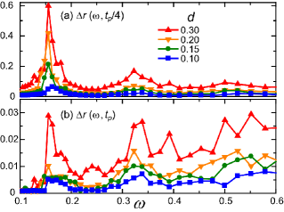
Figure 2: (Color online) Average displacement length ${\Delta r}(\omega,\tau)$ in Eq.(3) vs $\omega$ for (a) $\tau=t_{p}/4$ and (b) $\tau=t_{p}$ with $d=0.3,0.25,0.2$, and 0.1. Average is taken over 200 cycles for $t\geq 50t_{p}$. At $\omega\cong\omega_{1}$ reversibility is conspicuous in (a), but irreversibility increases with increasing $\omega$ in (b).

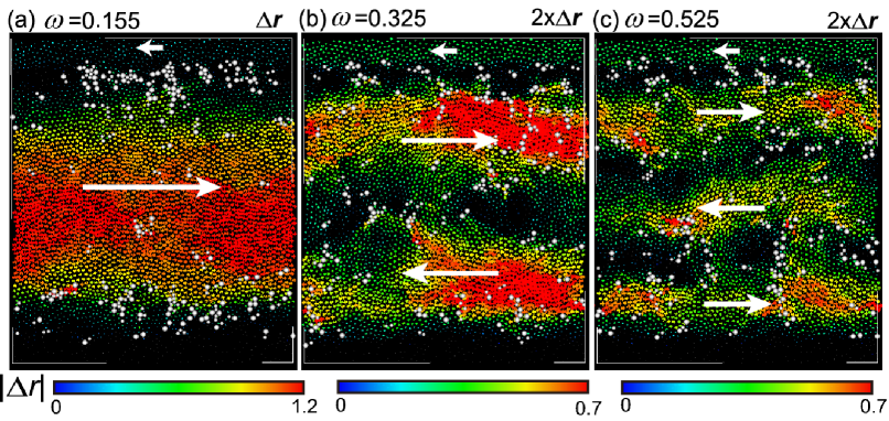
Figure 3: (Color online) Displacements $\Delta{\mbox{\boldmath$r$}}_{i}={\mbox{\boldmath$r$}}_{i}(nt_{p}+t_{p}/4)-{\mbox{\boldmath$r$}}_{i}(nt_{p})$ in a quarter cycle at $n\sim 100$ for $d=0.3$, where $\omega$ is (a) $\omega_{1}=0.155$, (b) $\omega_{2}=0.325$, and (c) $\omega_{3}=0.525$. Colors represent $|\Delta{\mbox{\boldmath$r$}}_{i}|$ according to the color bar. Particles in white are those with bonds broken in $[nt_{p},(n+1)t_{p}]$. White arrows are eye guides to show the average of $\Delta{\mbox{\boldmath$r$}}_{i}$ along the $x$ axis.

To describe plastic events, we here introduce the bond breakage Yamamoto for each cycle. Namely, particles $i$ and $j$ have broken bonds if their distance $r_{ij}(t)$ is shorter than $1.15\sigma_{\alpha\beta}$ at $t=nt_{p}$ and is longer than $1.25\sigma_{\alpha\beta}$ at $t=(n+1)t_{p}$. In Fig. 3, these particles are marked (in white). Then plastic events are visualized, which are collective and heterogeneous, taking place more frequently in regions with larger velocity gradients. Let $N_{\rm B}(\omega,n)$ be the number of these particles with broken bonds in the $n$-th cycle. Then, the energy dissipation at resonance fluctuates around $\epsilon N_{\rm B}(\omega,n)$ in each cycle comment1 . In fact, the averages of the one-cycle energy input $\Delta W(n)=W(nt_{p}+t_{p})-W(nt_{p})$ input and $\epsilon N_{\rm B}(\omega,n)$ over $n$ are both about $50\epsilon$ for $\omega=0.155$ and $d=0.3$.

Intermittency and big drop.– In Fig. 4(a), we show $N_{\rm B}(\omega,n)$ vs $n$ at $\omega=0.155$ in the range $n=t/t_{p}\leq 1300$. See its behavior on shorter time scales in SM Supp . It evolves intermittently for $n\lesssim 800$ but largely drops at $n\sim 800$. This drop indicates a transition from resonant to off-resonant states, which is similar to the absorbing transitions from active to inactive states Abs ; Pine ; Keim ; Berthier ; Sood . In (b), we plot the energy deviation $\Delta H(t)=\Delta K+\Delta U$ from its initial value at $\omega=0.155$, whose fluctuations greatly increase with increasing $d$. For $d=0.2$ and $0.3$, it drops to negative values ($-0.01N\epsilon$ and $-0.02N\epsilon$, respectively). The curves of $d=0.3$ in (a) and (b) are obtained from the same run. With the drop, cooling occurs to the boundary temperature 0.01 on time scales of $25-50t_{p}$. On the other hand, for $d=0.15$, $\Delta H$ decreases to a small positive value ($\sim 10^{-3}$), where a weakly resonant state follows. The time of these transitions is random depending on the initial state.

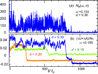
Figure 4: (Color online) Long time behaviors at $\omega=0.155$ for $n=t/t_{p}<1300$. (a) Particle number $N_{B}(\omega,n)$ with broken bonds vs $n$ for $d=0.3$, showing intermittency for $n\lesssim 800$. (b) Normalized deviation of energy $\Delta H/N\epsilon=(\Delta K+\Delta U)/N\epsilon$. Resonance disappears for $d=0.3$ at $n\sim 800$ and for $d=0.2$ at $n\sim 350$, while it is weakened for $d=0.15$ at $n\sim 550$.

Forced aging.– We show that the aging is accelerated during resonance Lacks ; Nagel . In Figs. 1 and 4(b), however, heating and amplified waves yield positive energy changes $\Delta H>0$ from the initial value. Thus, we switched off the oscillation after many resonant cycles and cooled the cell to 0.01 in an equilibration time of $10^{3}$. If we use the data of $d=0.3$ in Fig. 4 after $M$ cycles, $\Delta H$ is $-0.045N\epsilon$ for $M=600$ and is $-0.047N\epsilon$ for $M=1000$ after cooling. Furthermore, in Fig. 5(a), the shear modulus $G$ from the stress-strain relation (in units of $\epsilon\sigma_{1}^{-2}$) is 20 both in these two cases after cooling, which is considerably larger than the initial value $16$. Since the big drop is at $t/t_{p}\sim 800$ for $d=0.3$ in Fig. 4, the structure change leading to this hardening should have occurred before the big drop. If we again applied a periodic shear to these cooled states, resonance occurred at a higher frequency about $\pi(G/\rho)^{1/2}/L\cong 0.17$ (not shown here). Thus, the resonant states realized in simulation are history-dependent. For the run of $d=0.15$ in Fig. 4(b), $G$ increased only by 1 from its initial value.

At high-amplitude resonance, the waves are largely deformed on mesoscopic scales in considerably heated regions, where $G$ considerably depends on $T$ comment2 . Thus, the sound propagation in resonance is very complicated. Remarkably, at big drops breaking resonance, we observed exceptionally large plastic events and system-size sliding motions, as in Fig. 5(b). We conjecture that these large-scale motions break the resonance condition. In Fig. S4 in SM Supp , we will visualize smaller-scale sliding motions not breaking resonance. As a similar finding, Fiocco et al. Sastry numerically realized a thick shear band at large periodic strains. It is worth noting that long-range elastic deformations are produced around local plstic events Anael . We should further study these large-scale motions (in addition to plastic events) in sheared glass.

Diffusion.– The particles can jump out of cages appreciably at large strains even at very low $T$ Berthier ; Sastry ; Priez . This is consistent with our claim that the aging processes are accelerated at resonance. Here, we examine the stroboscopic mean square displacement along the $y$ axis in time intervals with width $nt_{p}$ written as

$$M(n)=\left\langle{\sum_{1\leq i\leq N}|{y}_{i}((n+s)t_{p})-{y}_{i}(st_{p})|^{2}/N}\right\rangle.$$ (4)

where the average is taken over $s$ ($0\leq s<100$) at fixed $n$. In Fig. 6, we plot $M(n)$ in the range $n<10^{3}$. For $d=0.3$, it grows as $4D_{\perp}nt_{p}$ for $n\gtrsim 20$, where the diffusion constant is given by $D_{\perp}=5.0\times 10^{-5}~{}\sigma_{1}^{2}/t_{0}$ diffusion .

For $d=0.15$ in Fig. 6, $M(n)$ remains close to its plateau, so it does not give $D_{\perp}$. Here, we note that the diffusion constant can be obtained from short-time analysis of jump motions in glass KawasakiPRE . To this end, we pick up the particles with large displacement $|{\mbox{\boldmath$r$}}_{i}((s+n)t_{p})-{\mbox{\boldmath$r$}}_{i}(st_{p})|>\ell_{\rm J}=0.8$, where $\ell_{\rm J}$ gives the first minimum of the Van Hove self-correlation function. Their contribution to $M(n)$ in Eq.(4) is written as

$$M_{\rm JP}(n)=\left\langle{\sum_{i\in{\rm jump}}|{y}_{i}((n+s)t_{p})-{y}_{i}(st_{p})|^{2}/N}\right\rangle.$$ (5)

where we remove the contribution from the thermal cage motions. Indeed, for $d=0.15$ in Fig. 6, we find $M_{\rm JP}(n)\cong 4D_{\perp}nt_{p}$ from small $n$ with $D_{\perp}=3.25\times 10^{-7}~{}\sigma_{1}^{2}/t_{0}$, where the jump number is of order $10^{-4}N$ per cycle and is small.

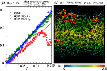
Figure 5: (Color online) (a) Stress $\sigma_{xy}$ vs strain $\gamma$ in three states at $T=0.01$. Initial slope of each curve gives the shear modulus $G$. It is 16 for the initial state in simulation. It is 20 for the other states obtained by switching-off the oscillation after $600$ and 1000 cycles in the run of $d=0.3$ in Fig. 4. (b) Displacements $\Delta{\mbox{\boldmath$r$}}_{i}$ in time interval $[750t_{p},850t_{p}]$ in the run of $d=0.3$ at $\omega=0.155$ in Fig. 4. Here, large plastic events and system-size sliding break resonance. Particles with $|\Delta{\mbox{\boldmath$r$}}_{i}|>2$ (in red) amount to 24 due to multiple stringlike motions.

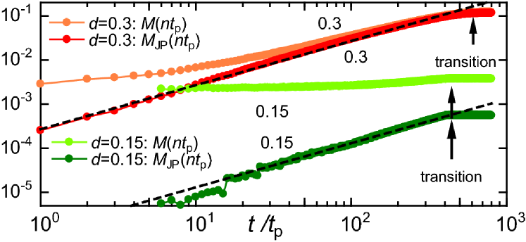
Figure 6: (Color online) Stroboscopic mean square displacement $M(n)$ and contribution to it from the particles with large jumps $M_{\rm JP}(n)$ as functions of $n=t/t_{p}<1000$ for $d=0.15$ and 0.3 at $\omega=0.155$. Here, $M(n)\propto D_{\perp}n$ at large $n$ only for $d=0.3$, but $M_{\rm JP}(n)\propto D_{\perp}n$ after several cycles even for $d=0.15$. They cease to increase after the big drop (arrow).

Summary.– We have examined acoustic resonance in a 2D model glass under periodic shear with amplitude $d$ and frequency $\omega$ applied at a wall. The resonant displacements can be very large even for small $d$. The damping arises from heterogeneous and intermittent plastic events. We have found resonance hardening (increase in the shear modulus $G$), which could be used in technological applications. Here, we predict that if we increase $\omega$ gradually depending on $G$, we can maintain resonance to achieve further hardening.

We still do not understand how the sound waves are emitted, deformed, and reflected in glass, where plastic events come into play at large amplitudes. See very complex wave behaviors in the movie in SM Supp . We should further examine how the resonance saturation occurs and how the structural changes proceed during resonance. We will also report on resonance of longitudinal sounds in glass by periodically changing the cell volume. For crystals and polycrystals, we should investigate how the resonance is influenced by the structural defects.

Supplementary Material

Acoustic resonance in periodically sheared glass

Takeshi Kawasaki¹ and Akira Onuki²

¹Department of Physics, Nagoya University, Nagoya 464-8602, Japan

²Department of Physics, Kyoto University, Kyoto 606-8502, Japan

I Early-stage time-evolution: caption of movie

In Fig. 1 of our Letter, we have shown resonant growth of the kinetic and potential energies for $d=0.30$ and $\omega=0.155$. Here, in Fig. S1(a), we obtain a periodically deformed state with small acoustic energy at off-resonance at $\omega=0.1$. We also explain the movie attached, which illustrates time evolution for $d=0.3$ and $\omega=0.155$ in the first ten cycles ($0<t<10t_{p}$). Depicted are the incremental changes of the particle positions,

$$\Delta{\mbox{\boldmath$r$}}_{i}(t,\Delta t)={\mbox{\boldmath$r$}}_{i}(t+\Delta t)-{\mbox{\boldmath$r$}}_{i}(t)\quad(t/\Delta t=0,1,2,\cdots,\quad t/t_{p}<10),$$ (S.1)

where $\Delta t=t_{p}/40\cong 1.0$. In (b), the kinetic energy deviation $\Delta K(t)$ consists of the oscillatory acoustic part and the slowly increasing thermal part due to heating, which are about $0.01N\epsilon$ and $0.02N\epsilon$, respectively, at $t/t_{p}\sim 10$. The random thermal motions within narrow cages change on a rapid time scale of $0.1$ and appear as small noises in $\Delta{\mbox{\boldmath$r$}}_{i}$. In the movie, the arrows with noticeable sizes can be identified as the acoustic velocities multiplied by $\Delta t$.

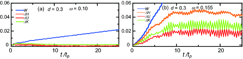
Figure S1: Deviations of kinetic energy $K$, potential energy $U$, and sum $K+U$ divided by $N\epsilon$ with $W(t)$ being energy input after application of periodic shear, where (a) $\omega=0.1$ with $d=0.30$ at off-resonance and (b) $\omega=\omega_{1}=0.155$ with $d=0.3$ at resonance. In (a) $\Delta K$ and $\Delta U$ remain small, while (b) corresponds to the movie attached.

II Eigenmodes with rigid walls

To understand the resonance we should also examine the vibrational normal modes from the Hessian matrix, where the eigenvectors should vanish at $y=0$ and $L$. To this end we included the 500 particles connected to the boundary walls (in the regions $-L/16<y<0$ and $L<y<17L/16$) by the spring potentials. We thus treated a 2D binary mixture of 4500 particles in a $L\times 9L/8$ rectangle with $L=70.2$, imposing the periodic boundary condition along the $x$ axis. We used the particle configuration obtained by cooling the state after $700$ resonant cycles for $d=0.3$ in Fig. 4 (see the explanation of Fig. 5(a)). This linear analysis itself is of interest, because the periodic boundary condition has been imposed along all the axes in the previous calculations of the vibrational modes (see Refs.$[22-26]$ in our Letter).

Figure S2: First 15 normal modes obtained from the Hessian matrix with the rigid boundary condition at $-L/16<y<0$ and $L<y<17L/16$ and the periodic boundary condition along the $x$ axis. Colors of the particles represent the displacement magnitude $|{\mbox{\boldmath$u$}}_{i}|$ of the corresponding eigenmode. Particle positions in the Hessian matrix are obtained from cooling the state at $t=700t_{p}$ with $d=0.3$ in Fig. 4(a). The first, second, and sixth shear modes are amplified in Fig. 3 in our Letter.

Our system is sufficiently large such that the first few extended sound modes have lower frequencies $\omega$ than those of the quasi-localized vibrations SchS . Thus, at low $\omega$, we can compare the eigenmodes from the Hessian matrix and the elastic modes from the linear elasticity (EMs). In the latter, the 2D displacement ${\mbox{\boldmath$u$}}=(u_{x},u_{y})$ obeys LandauS

$$-\rho\omega^{2}{\mbox{\boldmath$u$}}=B\nabla(\nabla\cdot{\mbox{\boldmath$u$}})+G\nabla^{2}{\mbox{\boldmath$u$}},$$ (S.2)

where $\rho$ is the mass density, $B$ is the bulk modulus, and $G$ is the shear modulus. Dissipation is neglected here. We solve this equation assuming the sinusoidal $x$ dependence ${\mbox{\boldmath$u$}}\propto e^{ik_{x}x}$ and the boundary condition ${\mbox{\boldmath$u$}}={\mbox{\boldmath$0$}}$ at $y=0$ and $L$ in the complex number representation.

First, for $k_{x}=0$, we obtain the transverse and longitudinal EMs:

$${\mbox{\boldmath$u$}}_{\ell}^{\rm T}=\sin(\pi\ell y/L){\mbox{\boldmath$e$}}_{x},\quad{\mbox{\boldmath$u$}}_{\ell}^{\rm L}=\sin(\pi\ell y/L){\mbox{\boldmath$e$}}_{y}\quad(\ell=1,2,\cdots),$$ (S.3)

where ${\mbox{\boldmath$e$}}_{x}$ and ${\mbox{\boldmath$e$}}_{y}$ are the unit vectors along the $x$ and $y$ axes, respectively. In terms of the sound speeds $c_{\perp}=(G/\rho)^{1/2}$ and $c_{\parallel}=[(B+G)/\rho]^{1/2}$, their eigenfrequencies are given by

$$\omega_{\ell}=\pi\ell c_{\perp}/L,\quad\omega_{\ell}^{\prime}=\pi\ell c_{\parallel}/L\quad(\ell=1,2,\cdots).$$ (S.4)

Here, $\pi$ is replaced by $2\pi$ in the periodic boundary condition along the $y$ axis. Second, let $k_{x}=2\pi/L$ in Eq. (S2). In this case, $u$ represents a mixed EM, since it can be expressed as

$$u_{x}=-\nabla_{y}H-ik_{x}J,\quad u_{y}=ik_{x}H-\nabla_{y}J,$$ (S.5)

where $\nabla_{y}=\partial/\partial y$. The two functions $H(y)$ and $J(y)$ satisfy $\nabla_{y}^{2}H=(k_{x}^{2}-\omega^{2}/c_{\perp}^{2})H$ and $\nabla_{y}^{2}J=(k_{x}^{2}-\omega^{2}/c_{\parallel}^{2})J$. This decomposition of $u$ into the transverse and longitudinal parts can be used to calculate the Rayleigh surface wave LandauS . In the range $\omega_{2}<\omega<\omega_{2}^{\prime}$ we set

$$H=H_{0}\cos[q_{\perp}(y-L/2)],\quad J=J_{0}\sinh[q_{\parallel}(y-L/2)]$$ (S.6)

where $(q_{\perp}/k_{x})^{2}=(\omega/\omega_{2})^{2}-1$ and $(q_{\parallel}/k_{x})^{2}=1-(\omega/\omega_{2}^{\prime})^{2}$ with $H_{0}$ and $J_{0}$ being constants. Here, $\omega$ is determined by $q_{\perp}q_{\parallel}/k_{x}^{2}=-\cot(q_{\perp}L/2)\tanh(q_{\parallel}L/2)$, which gives $\omega/\omega_{2}=1.17$ for $c_{\parallel}/c_{\perp}=3$, for example.

In Fig. S2, we display the first 15 eigenmodes of the Hessian matrix, which vanish at $y=0$ and $L$. The first two modes correspond to those of transverse EMs $(\ell=1,2)$. However, their frequencies $0.176$ and $0.360$ are somewhat higher than the resonant ones $0.155$ and $0.323$ in Figs. 2 and 3. The third and fourth modes are roughly proportional to $\cos(2\pi x/L+\alpha)$ and $\sin(2\pi x/L+\alpha)$ with $\alpha$ being a constant, so they correspond to the mixed EM ($\propto e^{2\pi ix/L}$) in Eq. (S5) with $\omega/\omega_{2}\sim 1.2$. In fact, $u_{x}$ is odd and $u_{y}$ is even as functions of $y-L/2$ for these modes. In the fifth mode, all the displacements of the particles are upward, so it corresponds to the first longitudinal EM, leading to $c_{\parallel}\cong 11$ from $\omega=\pi c_{\parallel}/L$. The sixth and ninth ones correspond to the third and fourth transverse EMs $(\ell=3$ and 4), but they largely vary in the $x$ direction. The seventh and eighth ones look similar to the sixth one, but are amplified at the middle ($y\sim L/2$). From the sixth to ninth modes, the excited regions form long stripes. The other ones vary in space both in the $x$ and $y$ directions in quasi-localized manners, where mesoscopic regions of large displacements are distinctly separated but are weakly connected SchS . In our case, all the eigenvectors from the Hessian matrix are extended in the whole cell. This aspect has not been well studied.

We also calculated the eigenvectors for the particle positions in the initial state of simulation and for those after 1000 cycles for $d=0.3$ in Fig. 4. The first 6 eigenvectors in these cases are nearly the same as those in Fig. S2, but the higher quasi-localized modes are significantly different. We can see that the quasi-localized modes sensitively depend on the details of the particle configurations. In the resonant states, they are also excited and mixed with the primary shear wave mode, but they vary in time with the structural changes.

III Periodic solution from linear elasticity

Let us calculate the periodic shear displacement $u_{x}(y,t)$ from the linear elasticity without damping LandauS , which can be realized after many cycles at off-resonance. Imposing the boundary conditions $u_{x}(0,t)=0$ and $u_{x}(L,t)=-d\sin(\omega t)$ in Eq. (2), we obtain

$$u_{x}=-d\sin(\omega t)\sin(\omega y/c_{\perp})/\sin(\omega L/c_{\perp}),$$ (S.7)

which diverges as $\omega\to\omega_{\ell}=\pi\ell c_{\perp}/L$, so we assume $\omega\neq\omega_{\ell}$. If $\omega\ll\omega_{1}$, this continuum expreesion is consistent with our simulation data far from the boundary walls on the average. Here, the acoustic energy $E_{a}$ is the space integral of $\rho({\partial u_{x}}/{\partial t})^{2}/2+G(\partial u_{x}/\partial y)^{2}/2$ in the linear elasticity. Therefore, if $E_{a}$ is averaged over one cycle, we obtain

$$\left\langle{E_{a}}\right\rangle=\frac{1}{t_{p}}\int_{0}^{t_{p}}dtE_{a}(t)=\rho L^{2}[d\omega/2\sin(\omega L/c_{\perp})]^{2}\quad(\omega\neq\omega_{\ell}).$$ (S.8)

For our model system, this gives $\left\langle{E_{a}}\right\rangle\cong 2.1\times 10^{-5}N\epsilon/(\omega/\omega_{\ell}-1)^{2}$ close to resonance for $d=0.15$, where the coefficient is very small. However, as Fig. 2 of our Letter indicates, the above expression holds only for $\omega\ll\omega_{1}$. Here, as $\omega\to 0$, $\left\langle{E_{a}}\right\rangle$ tends to $Gd^{2}/4$, where $G=\rho c_{\perp}^{2}$ is the shear modulus in the limit of low frequency and long wavelength.

IV Intermittency and collective motions

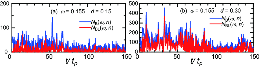
Figure S3: Particle numbers $N_{\rm B}(\omega,n)$ with broken bonds (in blue) and $N_{\rm BL}(\omega,n)$ with large jumps (in red) in time interval $[nt_{p},(n+1)t_{p}]$ vs $n=t/t_{p}$ at $\omega=0.155$ in the range $n=t/t_{p}<150$, where $d$ is (a) $0.15$ and (b) 0.3.

In Fig. 4(a), we have plotted the particle number $N_{\rm B}(\omega,n)$ with broken bonds in the $n$-th cycle at the first resonance $\omega=0.155$ for $d=0.3$ in the time range $n=t/t_{p}<1300$. In Fig. S3, we display its intermittent time evolution in the shorter range $n=t/t_{p}<150$ for $d=0.15$ and 0.3. Here, we should note that a considerable fraction of these particles with broken bonds return to their original positions in subsequent cycles, as has been reported in the off-resonant situations (see Refs.$[10-17]$ in our Letter). Hence, we also consider the particles with large displacement with $|{\mbox{\boldmath$r$}}_{j}(nt_{p}+t_{p})-{\mbox{\boldmath$r$}}_{j}(nt_{p})|>0.8$, as in Fig. 6 in our Letter KawasakiPRES . These particles have irreversibly escaped from cages and have also broken bonds in the n-th cycle, so their number ${N}_{\rm BL}(\omega,n)$ is smaller than or equal to ${N}_{\rm B}(\omega,n)$ in Fig. S3. Note that their jump motions give rise to translational diffusion as in Fig. 6.

In Fig. S4, we show snapshots of the irreversible displacements $\Delta r_{i}={\mbox{\boldmath$r$}}_{i}(nt_{p}+t_{p})-{\mbox{\boldmath$r$}}_{i}(nt_{p})$ for $d=0.3$ and $\omega=0.155$ in four consecutive cycles, where $n=t/t_{p}$ is (a) 23, (b) 24, (c) 25 and (d) 26. The distributions of the particles with broken bonds (in white) demonstrate intermittent fluctuations of the plastic events in successive cycles. Remarkably, in (a), (b), and (d), we can see large-scale collective motions with considerably large displacements ($\sim 0.5$ in (a)), while in (c) such collective motions are inconspicuous. During these cycles, the system remains at resonance. In Fig. 5(b), we have shown system-size sliding along the $x$ axis at $n\sim 800$ in the same run, which breaks resonance. Thus, large-scale collective motions of various sizes appear intermittently together with plastic events. We note that they may be treated as elastic deformations away from the particles with broken bonds. Indeed, long-range elastic strains have been calculated around local plastic events in glass AnaelS , which are similar to the Eshelby strains around precipitates in metallic alloys.

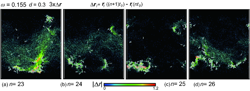
Figure S4: Snapshots of irreversible displacements $\Delta{\mbox{\boldmath$r$}}_{i}={\mbox{\boldmath$r$}}_{i}(nt_{p}+t_{p})-{\mbox{\boldmath$r$}}_{i}(nt_{p})$ for consecutive four cycles with $n=t/t_{p}=23,24,25$ and $26$, where $\omega=0.155$ and $d=0.3$. They largely fluctuate, because collective plastic events occur intermittently. Particles with broken bonds are drawn in while circles. We can see repeated plastic events in the lower region. Large-scale collective motions are also shown.

V Excitation of longitudinal waves

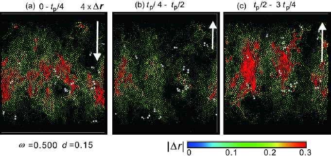
Figure S5: Resonance of longitudinal sounds induced by small periodic shear, where $\omega$ is increased in a stepwise manner up to $0.5$ with $d=0.15$. Depicted are $\Delta{\mbox{\boldmath$r$}}_{j}={\mbox{\boldmath$r$}}_{j}(t_{1}+t_{p}/4)-{\mbox{\boldmath$r$}}_{j}(t_{1})$ (multiplied by 4) in consecutive quarter cycles with width $t_{p}/4$, where $t_{1}$ is (a) $225t_{p}$, (b)$(225+1/4)t_{p}$, and (c) $(225+1/2)t_{p}$. Averages of $\Delta{\mbox{\boldmath$r$}}_{i}=(\Delta x_{i},\Delta y_{i})$ over all the particles are (a) $(0.07,-0.14)$, (b) $(0.003,0.095)$, and (c) $(-0.02,0.14)$ (white arrows).

In our Letter, we started with the same initial state and applied the periodic shear in Eq. (2) fixing $d$ and $\omega$ in each simulation run. We also performed simulation by increasing $\omega$ slowly in a stepwise manner at each fixed $d$, where we found considerably different resonance behavior at relatively high $\omega\gtrsim\omega_{2}$. In particular, we realized resonance of longitudinal sounds at $\omega\cong\pi c_{\parallel}/L\sim 0.5$ with $c_{\parallel}\sim 10$. In fact, in Fig. S5, we show amplified compression and expansion along the $y$ axis vanishing at the walls for $\omega=0.5$ with $d=0.15$. We can see that the particle displacements are mostly downward in (a) and upward in (b) and (c), though they are partially transverse varying along the $x$ axis. Therefore, the resonant behaviors are so complex in glass such that they even depend on the simulation path (protocol). In future work we will apply periodic dilation to glass to induce longitudinal wave resonance.

References

- (1) L.D. Landau and E.M. Lifshitz, Theory of Elasticity (Pergamon, New York,1973).
- (2) H. R. Schober and G. Ruocco, Philos. Mag. 84, 1361 (2004).
- (3) T. Kawasaki and A. Onuki, Phys. Rev. E 87, 012312 (2013).
- (4) A. Lemaître and C. Caroli, Phys. Rev. E 76, 036104 (2007).