Split energy cascade in turbulent thin fluid layers

Abstract

We discuss the phenomenology of the split energy cascade in a three-dimensional thin fluid layer by mean of high resolution numerical simulations of the Navier-Stokes equations. We observe the presence of both an inverse energy cascade at large scales, as predicted for two-dimensional turbulence, and of a direct energy cascade at small scales, as in three-dimensional turbulence. The inverse energy cascade is associated with a direct cascade of enstrophy in the intermediate range of scales. Notably, we find that the inverse cascade of energy in this system is not a pure 2D phenomenon, as the coupling with the 3D velocity field is necessary to guarantee the constancy of fluxes.

I Introduction

Fifty years ago, Kraichnan showed in the seminal paper Kraichnan (1967) that the dynamics of an incompressible flow in two-dimensions (2D) is dramatically different from the classical phenomenology of three-dimensional (3D) turbulence. The presence of two inviscid quadratic invariants, energy and enstrophy, gives rise to a double-cascade scenario Eyink (1996). At variance with the 3D case, in which the kinetic energy cascades toward small viscous scales, in 2D it is transferred toward large scales. Such “inverse energy cascade” is accompanied by a “direct enstrophy cascade”, which proceeds towards small scales Boffetta and Ecke (2012). In the inverse and direct ranges of scales the theory predicts a kinetic energy spectrum $E(k)\simeq\varepsilon_{f}^{2/3}k^{-5/3}$ and $E(k)\simeq\eta_{f}^{2/3}k^{-3}$ with possible logarithmic corrections Kraichnan (1971). Here and in the following $\varepsilon_{f}$ and $\eta_{f}$ denote the energy and the enstrophy injection rates respectively. The Kraichnan seminal concept of inverse cascade has become since then a prototypical model for several turbulent systems, from the inverse cascade in strongly rotating 3D flows Pouquet et al. (2013), to the inverse cascade of magnetic helicity in three-dimensional magneto-hydrodynamic turbulence Frisch et al. (1975), of passive scalar in compressible turbulence Chertkov et al. (1998), of wave action in weak turbulence Zakharov and Zaslavskii (1982).

The presence of the two cascades in two-dimensional turbulence has been observed in a number of numerical simulations Frisch and Sulem (1984); Herring and McWilliams (1985); Maltrud and Vallis (1991); Smith and Yakhot (1993); Boffetta et al. (2000, 2002); Chen et al. (2003); Xiao et al. (2009); Boffetta and Musacchio (2010); Cencini et al. (2011) and in experiments in soap films Rutgers (1998); Belmonte et al. (1999); Rivera et al. (1998); Rivera and Wu (2000, 2002); Bruneau and Kellay (2005); Rivera et al. (2014) and in thin fluid layers Paret and Tabeling (1997); Paret et al. (1999); Kellay and Goldburg (2002).

At variance with the numerical investigations, which allows to to study the ideal 2D Navier-Stokes equations, the experiments have to deal with the effects of the finite thickness of the fluid layer. This issue, which has been often considered a limitation for two-dimensional experiments, opens a series of interesting questions. How is the ideal 2D phenomenology modified in the case of a thin (3D) fluid layer? How thin should the layer be, in order to display the 2D-like double cascade? In which way does the transition from the 2D to the 3D regime occur at increasing the thickness of the layer?

These questions have been addressed both in numerical simulations Smith et al. (1996); Celani et al. (2010) and experiments Xia et al. (2011); Byrne et al. (2011) which have shown that the critical parameter which controls the cascade direction is the ratio $S=L_{z}/L_{f}$ of the thickness to the forcing scale. When $S\geq 1$ the flow is 3D at the forcing scale and the injected energy produces a direct cascade as in usual 3D turbulence. By decreasing $S$ one observes the phenomenon of cascade splitting with a fraction of the injected energy which goes to large scales and the remaining energy which flows to small scales Smith et al. (1996); Celani et al. (2010). For $S\ll 1$ the flux of the direct energy cascade is expected to scale as $S^{2}$. This prediction has been verified in shell models for quasi-two-dimensional turbulence Boffetta et al. (2011). Further reducing $S$, the cascade of energy towards small scale vanishes when the thickness $L_{z}$ reaches the Kolmogorov scale $L_{\nu}$ and the flow recovers the standard 2D phenomenology.

In the present paper we investigate the entanglement of 2D and 3D dynamics which occurs in a turbulent fluid layer by means of numerical simulations of the 3D Navier-Stokes equations in a confined domain with $L_{z}<L_{f}$ (and $L_{z}>L_{\nu}$). In agreement with previous findings, we observe the phenomenon of splitting of the energy cascade. By introducing a suitable decomposition of the velocity field, we show that the inverse cascade involves mainly the kinetic energy of the 2D modes, while the energy of the remnant 3D velocity is transferred toward the viscous scales. We also show that the development of the inverse energy cascade is associated with a partial conservation of the enstrophy in the intermediate range of scales $L_{z}<\ell<L_{f}$. Interestingly, we find that 3D modes play a relevant role in the the 2D phenomenology which is observed at large scales. In particular, the transport of the 2D modes by the 3D velocity is necessary to ensure a constant flux of energy in the inverse cascade as well as a constant flux of enstrophy in the range $L_{z}<\ell<L_{f}$.

The remaining of the paper is organized as follows. Section II introduces the Navier-Stokes equations and the decomposition of the velocity field in the 2D and 3D modes. In Section III we report the results of the numerical simulations. Section IV is devoted to the conclusions. In the Appendix A we derive a 2D model for the dynamics of a thin layer in the limit $L_{z}\to 0$.

II Navier-Stokes equations for a thin layer

We consider the dynamics of a three-dimensional thin layer of fluid, ruled by the Navier-Stokes equations for the velocity field ${\bm{u}}({\bm{x}},t)$:

$$\partial_{t}{\bm{u}}+{\bm{u}}\cdot{\bm{\nabla}}{\bm{u}}=-{\bm{\nabla}}p+\nu\Delta{\bm{u}}+{\bm{f}}$$ (1)

where $\nu$ is the kinematic viscosity, ${\bm{f}}$ is the external forcing, and the pressure $p$ is determined by the incompressibility constraint ${\bm{\nabla}}\cdot{\bm{u}}=0$. The flow is confined in a thin domain of size $L_{x}=L_{y}=rL_{z}$ with $r\gg 1$ and periodic boundary conditions in all the directions.

In absence of forcing and dissipation, (1) preserves the kinetic energy $E=(1/2)\langle|{\bm{u}}|^{2}\rangle$ (where $\langle...\rangle$ denotes average over the space). The energy balance in the forced-dissipated case reads:

$$\frac{dE}{dt}=\varepsilon_{f}-\varepsilon_{\nu}$$ (2)

where $\varepsilon_{\nu}=\nu\langle({\bm{\nabla}}{\bm{u}})^{2}\rangle$ is the energy dissipation rate due to the viscosity and $\varepsilon_{f}=\langle{\bm{f}}\cdot{\bm{u}}\rangle$ is the energy input provided by the external forcing.

The forcing provides also an input of enstrophy $Z=(1/2)\langle|{\bm{\omega}}|^{2}\rangle$, (${\bm{\omega}}={\bm{\nabla}}\times{\bm{u}}$ denotes the vorticity field) at the rate $\eta_{f}=\langle({\bm{\nabla}}\times{\bm{f}})\cdot{\bm{\omega}}\rangle$. At variance with the ideal 2D case, the enstrophy is not preserved by the full 3D inviscid dynamics, but it is produced by the vortex stretching mechanism Tennekes and Lumley (1972). The equation for the vorticity field is obtained by taking the curl of (1)

$$\partial_{t}{\bm{\omega}}+{\bm{u}}\cdot{\bm{\nabla}}{\bm{\omega}}={\bm{\omega}}\cdot{\bm{\nabla}}{\bm{u}}+\nu\Delta{\bm{\omega}}+{\bm{f}_{\omega}}$$ (3)

where ${\bm{f}_{\omega}}={\bm{\nabla}}\times{\bm{f}}$ and ${\bm{\omega}}\cdot{\bm{\nabla}}{\bm{u}}$ represents the vortex stretching term.

In order to highlight the presence of a 2D phenomenology in the 3D flow, it is useful to decompose the velocity field as ${\bm{u}}={\bm{u}}^{2D}+{\bm{u}}^{3D}$. The 2D mode ${\bm{u}}^{2D}=(u_{x}^{2D}(x,y),u_{y}^{2D}(x,y),0)$ is defined as the average along the $z$ direction of the $x$ and $y$ components of the velocity field ${\bm{u}}$, and it satisfies the 2D incompressibility condition $\partial_{x}u_{x}^{2D}+\partial_{y}u_{y}^{2D}=0$. In the Fourier space it corresponds to the mode $k_{3}=0$ of the horizontal velocity ${\bm{u}}^{2D}(k_{1},k_{2})=(u_{x}(k_{1},k_{2}),u_{y}(k_{1},k_{2}),0)$. The field ${\bm{u}}^{3D}$ is defined as the difference ${\bm{u}}^{3D}={\bm{u}}-{\bm{u}}^{2D}$. By the above definitions it is easy to show that the total energy decomposes into a 2D contribution $E^{2D}=(1/2)\langle|{\bm{u}}^{2D}|^{2}\rangle$ and a 3D contribution $E^{3D}=(1/2)\langle|{\bm{u}}^{3D}|^{2}\rangle$ as $E=E^{2D}+E^{3D}$. We notice that, beside the kinetic energy of the vertical velocity, $E^{3D}$ contains also the contributions of the modes $k_{3}\neq 0$ of the horizontal components of the velocity.

Similarly, the vorticity field can be decomposed as ${\bm{\omega}}=\omega^{2D}\hat{\bm{z}}+{\bm{\omega}}^{3D}$, where $\omega^{2D}=\partial_{x}u_{y}^{2D}-\partial_{y}u_{x}^{2D}$ is the scalar vorticity of the two-dimensional flow. In the limit of vanishing thickness $L_{z}\to 0$ (at finite viscosity $\nu$) the vertical dependence disappears and ${\bm{u}}^{2D}$ becomes solution of the 2D Navier-Stokes equation (see Appendix A). Therefore, it is reasonable to assume that the occurrence of an inverse energy cascade at finite thickness $L_{z}$ should be associated to the dynamics of the 2D mode ${\bm{u}}^{2D}$.

III Direct numerical simulations

We performed a direct numerical simulation of the Navier-Stokes equations (1) in a confined geometry with periodic boundary conditions. The computational domain has dimensions $L_{x}=L_{y}=2\pi$, $L_{z}=L_{x}/64$ ($r=64$) and it is discretized on a uniform grid at resolution $N_{x}\times N_{y}\times N_{z}=4096\times 4096\times 64$. The numerical simulations are performed by means of a fully-parallel, pseudospectral code, with $2/3$ dealiasing scheme. We adopt an hyperviscous damping scheme $(-1)^{p-1}\nu_{p}\Delta^{p}$ with $p=4$ and $\nu_{p}=10^{-21}$. We do not use any large-scale dissipation (such as linear friction).

The flow is sustained by a “two-components, two-dimensional” forcing, that is, the forcing is active on the horizontal components of the velocity and it is dependent on the horizontal coordinates only, ${\bm{f}}=(f_{x}(x,y),f_{y}(x,y),0)$. Therefore in the vorticity equation (3) forcing ${\bm{f}}_{\omega}$ is active on the 2D field $\omega^{2D}$ only. Forcing is restricted to a narrow wavenumber shell in Fourier space with $k_{h}=(k_{1}^{2}+k_{2}^{2})^{1/2}\simeq k_{f},k_{3}=0$. Here $k_{f}=16$. The forcing is Gaussian and $\delta$-correlated in time to control the injection rates $\varepsilon_{f}$ and $\eta_{f}$. The characteristic time at the forcing scale is defined as $\tau_{f}=\eta_{f}^{-1/3}$. The ratio between the thickness $L_{z}=2\pi/k_{z}$ and the forcing scale $L_{f}=2\pi/k_{f}$ is $S=L_{z}/L_{f}=4$ This ensures the regime of split cascade with the coexistence of the 3D and the 2D phenomenology (see Fig. 1) Celani et al. (2010).

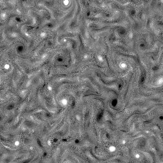
Figure 1: Snapshot of the scalar vorticity field $\omega^{2D}$ in the late stage of the simulation. Typical two-dimensional objects, such as strong vortices at the forcing scale $L_{f}$, coexist with small scale three-dimensional features.

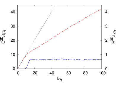
Figure 2: Temporal evolution of the kinetic energy $E^{2D}$ (red, dashed line, left $y$-axis) and $E^{3D}$ (blue, solid line, right $y$-axis). The dotted line represents the linear growth with the input rate $\varepsilon_{f}$ (left $y$-axis).

The velocity field at time $t=0$ is initialized to zero, plus a small random perturbation, which is required to trigger the 3D instability. The results shown in this Section has been obtained with an energy of the initial perturbation $E_{pert}\simeq 1.6\cdot 10^{-7}\varepsilon_{f}\tau_{f}$.

Because of the purely 2D forcing, in the early stage of the simulation ($t<10\tau_{f}$), the energy accumulates in the 2D mode ${\bm{u}}^{2D}$ at a rate equal to the forcing input, while the energy $E^{3D}$ of the 3D component is negligible (see Figure 2). The activation of the 3D modes ${\bm{u}}^{3D}$ (at $t\simeq 10\tau_{f}$) is accompanied by a significant reduction of the growth rate of the 2D energy as some of the injected energy is now transferred to small scales. At later times, $E^{3D}$ saturates to a statistically steady value (as in standard 3D turbulence), while the two-dimensional component $E^{2D}$ energy keeps increasing with a constant reduced rate $\varepsilon_{\alpha}<\varepsilon_{f}$. We stop the simulation at time $t=100\tau_{f}$, when the inverse energy cascade has reached the lowest wavenumber (see Figure 4). Continuing the simulation for further times, in absence of large-scale dissipation, we expect that the kinetic energy will accumulate in the lowest mode, giving rise to the so called “condensate”  Chertkov et al. (2007); Xia et al. (2009); Laurie et al. (2014). The 2D mode contains almost all the kinetic energy of the horizontal velocities, and the kinetic energy of the vertical component $u_{z}$ contained in the mode $k_{3}=0$ represents only $24\%$ of the total.

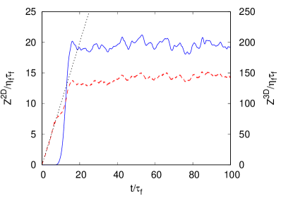
Figure 3: Temporal evolution of the enstrophy of $\omega^{2D}$ (red, dashed line, left $y$-axis) and ${\bm{\omega}}^{3D}$ (blue, solid line, right $y$-axis). The dotted line represents the linear growth with the input rate $\eta_{f}$ (left $y$-axis).

The enstrophy of the 2D mode $Z^{2D}=1/2\langle(\omega^{2D})^{2}\rangle$ grows initially with the input rate $\eta_{f}$, reflecting the pure 2D nature of the initial flow (see Figure 3). As 3D motions develop (at $t\simeq 10\tau_{f}$), the enstrophy associated to the 3D modes $Z^{3D}=1/2\langle|{\bm{\omega}}^{3D}|^{2}\rangle$ increases very rapidly and reaches a stationary value which is much larger than the saturation level of $Z^{2D}$.

III.1 Energy spectra

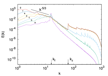
Figure 4: Energy spectra $E(k,t)$ at times $t/\tau_{f}=$ $4.6$ (a, violet), $6.9$ (b, green), $9.2$ (c, cyan), $13.7$ (d, orange), $18.3$ (e, yellow), $45.8$ (f, blue), $91.6$ (g, red). The last three spectra are almost superposed for $k>k_{z}$.

In Figure 4 we show the instantaneous spectra $E(k,t)$ of the total energy at different times $t$. The initial spectra are almost completely 2D, because the forcing is active only on 2D modes. We observe that the 3D instability begins at high harmonics of the thickness wavenumber $k_{z}$, then it propagates to all the modes $k>k_{z}$. The energy spectrum at $k>k_{f}$ saturates at time $t\simeq 16\tau_{f}$. At scales larger than the forcing scale, $k<k_{f}$, we observe the development of an inverse energy cascade with a power-law spectrum $E(k)\simeq\varepsilon_{\alpha}^{2/3}k^{-5/3}$.

The “spiky” aspect of the energy spectrum at high wavenumbers $k>k_{z}$ is due to the anisotropic spacing of the wavenumbers in the Fourier space. The separation between the discrete wavenumbers in the horizontal direction is $\Delta k_{h}=2\pi/L_{x}$ while in the vertical direction it is $\Delta k_{3}=2\pi/L_{z}=k_{z}$. Given that $L_{z}\ll L_{x}$, the wavenumber space is structured as horizontal dense layers, separated by large gaps in the vertical direction. Because the complete energy spectrum is defined as the integral of the square amplitude of the modes over a spherical wavenumber shell of radius $k$, one gets a sudden increase of the spectrum each time the spherical shell is a multiple of $k_{z}$.

In order to analyze the contribution of the 2D mode to the total energy spectrum, it is interesting also to consider the 2D spectra $E^{2D}(k)$, in which the integral is restricted to the horizontal wavenumbers $k_{h}=\sqrt{k_{1}^{2}+k_{2}^{2}}$ on the plane $k_{3}=0$. In physical space, this is equivalent of averaging first the velocity fields in the vertical direction $z$ and then computing the spectrum of the averaged 2D fields. It is worth to notice that, for $k<k_{z}$, the 2D spectra and 3D spectra coincide, because the spherical shell of radius $k<k_{z}$ intersects the planes $k_{3}=\pm mk_{z}$ only for $m=0$.

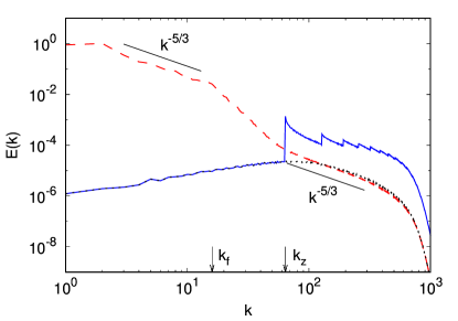
Figure 5: Energy spectrum $E^{2D}(k)$ of the 2D mode ${\bm{u}}^{2D}$ (red, dashed line) and 3D mode ${\bm{u}}^{3D}$ (blue, solid line). We also show the 2D spectrum of the vertically-averaged vertical velocity $u_{z}$ (black, dotted line). The spectra are computed at $t=100\tau_{f}$

In Figure 5 we compare the 2D energy spectrum $E^{2D}(k)$ of the 2D mode ${\bm{u}}^{2D}$ with the 3D energy spectrum of the 3D mode ${\bm{u}}^{3D}$. At low wavenumbers $k<k_{z}$ almost all the kinetic energy is contained in the 2D mode. This confirms that the inverse cascade which develops in the range $k<k_{f}$ concerns only the 2D energy. Conversely, the 3D mode contains the largest fraction of the kinetic energy at high wavenumbers $k>k_{z}$. Interestingly, in the same range of wavenumber, the 2D spectrum of the 2D mode displays a $-5/3$ slope, and it is very close to the 2D spectrum of the vertical component $u_{z}$.

The spectrum $E^{2D}(k)$ shown in Fig. 5 is reminescent of the horizontal spectrum (of meridional and zonal winds) observed in the upper troposphere by the Global Atmospheric Sampling Program Nastrom and Gage (1985) where a transition from a $k^{-3}$ to a $k^{-5/3}$ spectrum at small scales is observed. We remark that, despite the similarities between the two spectra, the physical mechanisms are probably different (see, for example, Lilly (1983), Vallgren et al. (2011)) as the transition in the atmospheric spectrum is observed at a scale around $500\,km$, while in our simulations it occours at a scale comparable with tickness of the layer.

III.2 Spectral fluxes

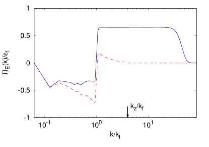
Figure 6: Spectral energy flux $\Pi_{E}(k)$ (blue solid line) and 2D energy flux (red, dashed line), at $t=100\tau_{f}$

The analysis of the spectral flux of the total kinetic energy $\Pi_{E}(k)$ shows that in a thin fluid layer the energy injected by the forcing at the wavenumber $k_{f}$ indeed splits in two parts (see Figure 6). At low wavenumbers $k<k_{f}$ we observe a constant, negative flux of energy, which indicates the presence of an inverse energy transfer toward large scales. At high wavenumbers $k>k_{f}$ we also observe a constant energy flux, now positive, indicating a direct cascade of energy toward small scales. It is worth to remind that the kinetic energy transported in the direct cascade is not only that of the vertical component of the velocity, but contains also the contributions of the modes $k_{3}\neq 0$ of the horizontal velocities. In this range of scales the dynamics in the vertical and horizontal directions is strongly coupled, and the positive energy flux cannot be explained in terms of a direct cascade of the vertical velocity passively transported by a two-dimensional, three components (2D3C) flow Campagne et al. (2014); Moffatt (2014); Biferale et al. (2017).

As we have shown in Fig. 4, the inverse cascade involves mainly the energy of the 2D mode. This observation suggests to check whether or not this inverse cascade coincides with a pure 2D dynamics of the 2D mode ${\bm{u}}^{2D}$. To this purpose we have taken the fields ${\bm{u}}^{2D}$ and we have truncated them at $k_{h}=k_{z}$ by setting to zero all the modes with $k_{h}>k_{z}$. Then, we have computed the 2D spectral fluxes of the truncated 2D fields, assuming that they were solutions of the two-dimensional Navier-Stokes equations. Surprisingly, we find that the 2D energy flux in the range of scales of the inverse cascade does not coincide with the 3D flux shown in Fig. 5. The physical interpretation of this result is that the energy of the 2D mode is not simply transported toward large scales by the 2D flow itself, but the 3D modes contribute to the transport process. This contrasts with a 2D3C scenario at large scales, with the vertical velocity being passively transported by the 2D flow  Campagne et al. (2014); Moffatt (2014); Biferale et al. (2017).

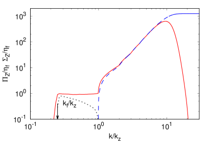
Figure 7: Spectral enstrophy flux $\Pi_{Z}(k)$ (red solid line), Spectral enstrophy production $\Sigma_{Z}(k)$ (blue, dashed line), and 2D enstrophy flux (black, dotted line), at $t=100\tau_{f}$

As discussed in Section II, the main difference between 3D and 2D Navier-Stokes equations is the absence of the vortex stretching term ${\bm{\omega}}\cdot{\bm{\nabla}}{\bm{u}}$ in the latter. The presence of two positive-defined inviscid invariants (energy and enstrophy) causes the reversal of the direction of the energy cascade. Even if the enstrophy is not conserved by the 3D dynamics, it is tempting to conjecture that the development of the inverse cascade in thin fluid layers is due to a dynamical suppression of the enstrophy production. To investigate this issue we computed the total spectral enstrophy flux $\Pi_{z}(k)$ and the total spectral enstrophy production $\Sigma_{Z}(k)$ defined as:

$$\Pi_{Z}=\int_{|\bm{q}|\leq{k}}d\bm{q}(\bm{v}\cdot\nabla\bm{\omega})(\bm{q})\bm{\omega}^{\ast}(\bm{q})\,,$$ (4)

$$\Sigma_{Z}=\int_{|\bm{q}|\leq{k}}d\bm{q}(\bm{\omega}\cdot\nabla\bm{v})(\bm{q})\bm{\omega}^{\ast}(\bm{q})\,.$$ (5)

In the range of wavenumbers $k_{f}<k<k_{z}$ the production of enstrophy is negligible, and the enstrophy flux is constant, as shown in Fig. 7. This constant flux corresponds to the presence of a direct enstrophy cascade. At high wavenumbers, $k>k_{z}$, the enstrophy production becomes significant and therefore the enstrophy flux is not constant anymore but grows following the production term. Our results show that, in analogy with the case of ideal 2D Navier-Stokes equations, also in a thin fluid layer the emergence of the inverse energy cascade is due to the presence of a “quasi invariant”, the enstrophy, which is conserved by the large-scale dynamics. Nonetheless, it is worth to notice, that the conservation of the enstrophy is not due to the transport by the 2D mode itself. Following the same procedure described in the case of the energy flux, we have computed the 2D enstrophy flux from the truncated 2D velocity fields. In the range of scale $k_{f}<k<k_{z}$ the 2D flux is positive, but not constant, thus indicating that the full 3D dynamics is required for the conservation of enstrophy (see Fig. 7).

The presence of an intermediate direct enstrophy cascade in the range of scales $L_{z}<\ell<L_{f}$ allows to derive a simple dimensional argument for the scaling of the energy flux toward small scales. A direct cascade with constant enstrophy flux $\eta_{f}=\varepsilon_{f}k_{f}^{2}$ carries also a residual energy flux, which decreases as $\Pi(k)\sim\varepsilon_{f}(k_{f}/k)^{2}$. By assuming that the flux of energy of the direct cascade which starts from $k_{z}$ is equal to the residual flux $\Pi(k_{z})$ carried by the enstropy cascade at the scale $k_{z}$, one gets the prediction $\varepsilon_{\nu}=\Pi(k_{z})\sim\varepsilon_{f}S^{2}$. This prediction has been verified in shell models for quasi-two-dimensional turbulence Boffetta et al. (2011).

IV Conclusions

In this paper we present a numerical study of the phenomenology of a turbulent flow confined in a thin fluid layer. We discuss the possibility to disentangle the complex mixture of 2D and 3D dynamics by a suitable decomposition of the velocity field in 2D and 3D modes.

In analogy with previous studies Smith et al. (1996); Celani et al. (2010), when the flow is forced at scales $L_{f}$ larger that the thickness $L_{z}$ of the layer we observe a splitting of the energy cascade in two directions. A fraction of the energy is transported toward large scale, giving rise to an inverse energy cascade, while the remnant energy is transported toward the small viscous scales, as in 3D turbulence. We show that the inverse energy cascade is accompanied by the development of a direct cascade of enstrophy in the intermediate range of scales $L_{z}<\ell<L_{f}$. The enstrophy production becomes relevant only at small scales $\ell<L_{z}$, allowing for a partial conservation of the enstrophy by the large-scale dynamics.

The scenario which emerges from our findings is a coexistence of 2D phenomenology, with a double cascade of energy and enstrophy à la Kraichnan at large scales $\ell>L_{z}$ and a 3D direct energy cascade à la Kolmogorov at small scales $\ell<L_{z}$. Interestingly, the decomposition of the velocity field in the 2D modes and the remaining 3D part reveals that the 2D and 3D dynamics are deeply entangled. On one hand, we find that the energy and enstrophy which are involved in the double cascade at large scales are those of the 2D modes. On the other hand, the 3D velocity is necessary to guarantee a constant flux of 2D energy and enstrophy in the large-scale transport.

We plan to extend the analysis of the interactions between 2D and 3D modes to the case of rotating and stably stratified thin fluid layers. Previous results Deusebio et al. (2014) shows that rotation causes a suppression of the enstrophy production similar to the effects of confinement, favoring the two-dimensionalization of the flow and the development of the inverse energy cascade. Nonetheless, this effect is not accompanied by the presence of a range of scales in which the enstrophy is conserved by the large-scale dynamics. This is likely to affect the interactions between 2D and 3D modes. In the case of stably stratified fluid layers, it has been shown that the conversion of kinetic energy into potential energy, which is promptly transferred toward the small diffusive scales, provides a fast dissipative mechanism which suppresses the large scale energy transfer Sozza et al. (2015). Investigating the interactions between 2D vortical modes and 3D potential modes will improve the understanding of this process.

Appendix A 2D model for thin layers

In this Appendix we discuss a two-dimensional model to describe the dynamics of a thin layer in which the both the thickness $L_{z}$ and the Kolmogorov scale $L_{\nu}$ tend to zero, but their ratio remains of order unity.

We consider Navier-Stokes equations (1) in a box in which the horizontal dimensions $L_{x}=L_{y}=L$ are much larger than the vertical thickness $L_{z}=\epsilon L$. The aspect ratio of the box is determined by the ratio $\epsilon=L_{x}/L_{z}$. We assume periodic b.c. in all the directions. We assume also that the external force ${\bm{f}}$ acts only on horizontal components and depends only on horizontal coordinates: ${\bm{f}}({\bm{x}})=(f_{x}(x,y),f_{y}(x,y),0)$.

The assumption that the thickness $L_{z}$ of the layer is very small and it is of the order of the viscous scale, allows to suppose that the modes $k_{3}>k_{z}$ are suppressed by the viscosity, and can be neglected. Therefore we make a Fourier truncation in the vertical direction by retaining only the first modes in the vertical direction $k_{3}=0,\pm k_{z}$ where $k_{z}=2\pi/L_{z}=O(\epsilon^{-1})$. The velocity fields can be expanded as

$$u_{l} = u^{0}_{l}+\sqrt{2}\left[u_{l}^{c}\cos(k_{z}z)+u_{l}^{s}\sin(k_{z}z)\right]\;$$ (6)

$$u_{3} = u^{0}_{3}+\sqrt{2}\left[u_{3}^{c}\cos(k_{z}z)+u_{3}^{s}\sin(k_{z}z)\right]\;.$$ (7)

where $l\in[1,2]$. Within this notation, the 2D mode ${\bm{u}}^{2D}$ introduced in Sec. II coincides with the field ${\bm{u}}^{0}=(u_{1}^{0},u_{2}^{0})$.

The incompressibility condition $\nabla\cdot{\bm{u}}=0$ gives:

$$\partial_{l}u_{l}^{0}=0\;;\;\partial_{l}u_{l}^{c}=-k_{z}u_{3}^{s}\;;\;\partial_{l}u_{l}^{s}=k_{z}u_{3}^{c}\;.$$ (8)

This shows that the 2D mode ${\bm{u}}^{0}$ satisfies the 2D incompressibility. The fields $u_{3}^{s,c}$ are determined by the compressibility of the fields ${\bm{u}}_{l}^{s,c}$. Expanding at leading order in $\epsilon$ the Navier-Stokes equations (1) one obtains the equations for the fields $u_{l}^{0}$,$u_{l}^{s,c}$ and $u_{3}^{0}$:

$$\partial_{t}u^{0}_{l}+u^{0}_{n}\partial_{n}u^{0}_{l} = -\partial_{l}p+\nu\partial_{n}\partial_{n}u^{0}_{l}+f_{l}$$

$$-\partial_{n}(u^{c}_{n}u^{c}_{l}+u^{s}_{n}u^{s}_{l})$$

$$\partial_{t}u^{c}_{l}+u^{0}_{n}\partial_{n}u^{c}_{l} = \nu\partial_{n}\partial_{n}u^{c}_{l}-\alpha u^{c}_{l}$$

$$-u^{c}_{n}\partial_{n}u^{0}_{l}+u^{0}_{3}k_{z}u^{s}_{l}$$

$$\partial_{t}u^{s}_{l}+u^{0}_{n}\partial_{n}u^{s}_{l} = \nu\partial_{n}\partial_{n}u^{s}_{l}-\alpha u^{s}_{l}$$

$$-u^{s}_{n}\partial_{n}u^{0}_{l}-u^{0}_{3}k_{z}u^{c}_{l}$$

$$\partial_{t}u^{0}_{3}+u^{0}_{n}\partial_{n}u^{0}_{3} = \nu\partial_{n}\partial_{n}u^{0}_{3}$$

$$+\left(u^{c}_{n}\partial_{n}\partial_{l}u^{s}_{l}-u^{s}_{n}\partial_{n}\partial_{l}u^{c}_{l}\right)/k_{z}\;,$$

where $l,n\in[1,2]$ and summation over repeated indices is assumed.

The linear friction term $-\alpha{\bm{u}}^{s,c}$ in the 2D model comes from the derivatives in the vertical direction of the viscous term in Eq. (1). At finite viscosity $\nu$, in the limit $k_{z}\to\infty$ the friction coefficient $\alpha=\nu k_{z}^{2}$ diverges. The modes ${\bm{u}}^{c,s}$ are therefore exponentially suppressed. In this limit, the equation for the 2D mode ${\bm{u}}^{0}$ reduces to the two-dimensional Navier-Stokes equations.

It is interesting also to consider the limit $k_{z}\to\infty$, in which the viscosity vanishes as $\nu\sim k_{z}^{-2}\to 0$ such that $\alpha=\nu k_{z}^{2}\to const$. In this case, the 2D mode ${\bm{u}}^{0}$ remains coupled with the 3D modes ${\bm{u}}^{s,c}$. The latters are transported and stretched by the gradients of the velocity field ${\bm{u}}^{0}$ and are coupled among themselves as an harmonic oscillator whose frequency is determined by the scalar field $u^{0}_{3}$.

The stretching of the fields ${\bm{u}}^{s,c}$ is contrasted by the linear relaxation term $-\alpha{\bm{u}}^{s,c}$. If the dissipation prevails the two fields are exponentially damped, and their feedback on the 2D velocity field ${\bm{u}}^{0}$ can be neglected. Conversely, when stretching dominates, part of the kinetic energy is transferred to the fields ${\bm{u}}^{s,c}$ and it is dissipated by the friction. The transition between the two regimes is expected to occur when $\lambda\sim\alpha$, where $\lambda$ is a suitable measure of the intensity of the gradients of the 2D mode. A dimensional estimate based on the scaling laws of the direct enstrophy cascade gives $\lambda\sim\eta_{f}^{1/3}$ where $\eta_{f}$ is the enstrophy flux. Recalling that the viscous scale $L_{\nu}$ (defined as the scale at which $Re=1$ ) is $L_{\nu}=\nu^{1/2}\eta_{f}^{-1/6}$ and that $\alpha\sim\nu L_{z}^{-2}$, the condition $\lambda>\alpha$ for the transition is equivalent to $L_{z}>L_{\nu}$. This shows that 3D modes can be excited only when the thickness $L_{z}$ is larger than the viscous scale $L_{\nu}$.

The development of the 3D modes causes a reduction of the growth rate of the 2D mode. This can be seen from the energy balance of the 2D model:

$$\frac{d}{dt}(E^{2D}+E^{3D})=\varepsilon_{f}-2\alpha E^{3D}$$ (13)

where $E^{2D}=1/2\langle|{\bm{u}}^{0}|^{2}\rangle$ is the energy of the 2D mode and $E^{3D}=1/2\langle|{\bm{u}}^{c}|^{2}+|{\bm{u}}^{s}|^{2}\rangle$ is the energy of the 3D modes. For $L_{z}>L_{\nu}$ the $E^{3D}$ attains a positive, statistically constant value, and therefore the growth rate $dE^{2D}/dt$ reduces to $\varepsilon_{\alpha}=\varepsilon_{f}-2\alpha E^{3D}<\varepsilon_{f}$.

We notice that the model does not provide a quantitative estimate of the energy $E^{3D}$ which appears in Eq. 13, and therefore it is not possible to determine the scaling dependence of the growth rate of $E^{2D}$ on the ratio $L_{z}/L_{\nu}$.

References

- Kraichnan (1967) R. H. Kraichnan, Phys. Fluids 10, 1417 (1967).
- Eyink (1996) G. L. Eyink, Physica D 91, 97 (1996).
- Boffetta and Ecke (2012) G. Boffetta and R. E. Ecke, Annu. Rev. Fluid Mech. 44, 427 (2012).
- Kraichnan (1971) R. H. Kraichnan, J. Fluid Mech. 47, 525 (1971).
- Pouquet et al. (2013) A. Pouquet, A. Sen, D. Rosenberg, P. D. Mininni, and J. Baerenzung, Phys. Scripta 2013, 014032 (2013).
- Frisch et al. (1975) U. Frisch, A. Pouquet, J. Léorat, and A. Mazure, J. Fluid Mech. 68, 769 (1975).
- Chertkov et al. (1998) M. Chertkov, I. Kolokolov, and M. Vergassola, Phys. Rev. Lett. 80, 512 (1998).
- Zakharov and Zaslavskii (1982) V. Zakharov and M. Zaslavskii, Izv. Atmos. Ocean. Phys. 18, 747 (1982).
- Frisch and Sulem (1984) U. Frisch and P.-L. Sulem, Phys. Fluids 27, 1921 (1984).
- Herring and McWilliams (1985) J. Herring and J. McWilliams, J. Fluid Mech. 153, 229 (1985).
- Maltrud and Vallis (1991) M. Maltrud and G. Vallis, J. Fluid Mech. 228, 321 (1991).
- Smith and Yakhot (1993) L. M. Smith and V. Yakhot, Phys. Rev. Lett. 71, 352 (1993).
- Boffetta et al. (2000) G. Boffetta, A. Celani, and M. Vergassola, Phys. Rev. E 61, R29 (2000).
- Boffetta et al. (2002) G. Boffetta, A. Celani, S. Musacchio, and M. Vergassola, Phys. Rev. E 66, 026304 (2002).
- Chen et al. (2003) S. Chen, R. E. Ecke, G. L. Eyink, X. Wang, and Z. Xiao, Phys. Rev. Lett. 91, 214501 (2003).
- Xiao et al. (2009) Z. Xiao, M. Wan, S. Chen, and G. Eyink, J. Fluid Mech. 619, 1 (2009).
- Boffetta and Musacchio (2010) G. Boffetta and S. Musacchio, Phys. Rev. E 82, 016307 (2010).
- Cencini et al. (2011) M. Cencini, P. Muratore-Ginanneschi, and A. Vulpiani, Phys. Rev. Lett. 107, 174502 (2011).
- Rutgers (1998) M. A. Rutgers, Phys. Rev. Lett. 81, 2244 (1998).
- Belmonte et al. (1999) A. Belmonte, W. Goldburg, H. Kellay, M. Rutgers, B. Martin, and X. Wu, Phys. Fluids 11, 1196 (1999).
- Rivera et al. (1998) M. Rivera, P. Vorobieff, and R. E. Ecke, Phys. Rev. Lett. 81, 1417 (1998).
- Rivera and Wu (2000) M. Rivera and X.-L. Wu, Phys. Rev. Lett. 85, 976 (2000).
- Rivera and Wu (2002) M. Rivera and X.-L. Wu, Phys. Fluids 14, 3098 (2002).
- Bruneau and Kellay (2005) C. H. Bruneau and H. Kellay, Phys. Rev. E 71, 046305 (2005).
- Rivera et al. (2014) M. Rivera, H. Aluie, and R. Ecke, Phys. Fluids 26, 055105 (2014).
- Paret and Tabeling (1997) J. Paret and P. Tabeling, Phys. Rev. Lett. 79, 4162 (1997).
- Paret et al. (1999) J. Paret, M.-C. Jullien, and P. Tabeling, Phys. Rev. Lett. 83, 3418 (1999).
- Kellay and Goldburg (2002) H. Kellay and W. I. Goldburg, Report Prog. Phys. 65, 845 (2002).
- Smith et al. (1996) L. M. Smith, J. R. Chasnov, and F. Waleffe, Phys. Rev. Lett. 77, 2467 (1996).
- Celani et al. (2010) A. Celani, S. Musacchio, and D. Vincenzi, Phys. Rev. Lett. 104, 184506 (2010).
- Xia et al. (2011) H. Xia, D. Byrne, G. Falkovich, and M. Shats, Nature Phys. 7, 321 (2011).
- Byrne et al. (2011) D. Byrne, H. Xia, and M. Shats, Phys. Fluids 23, 095109 (2011).
- Boffetta et al. (2011) G. Boffetta, F. De Lillo, and S. Musacchio, Phys. Rev. E 83, 066302 (2011).
- Tennekes and Lumley (1972) H. Tennekes and J. L. Lumley, A first course in turbulence (MIT press, 1972).
- Chertkov et al. (2007) M. Chertkov, C. Connaughton, I. Kolokolov, and V. Lebedev, Phys. Rev. Lett. 99, 084501 (2007).
- Xia et al. (2009) H. Xia, M. Shats, and G. Falkovich, Phys. Fluids 21, 125101 (2009).
- Laurie et al. (2014) J. Laurie, G. Boffetta, G. Falkovich, I. Kolokolov, and V. Lebedev, Phys. Rev. Lett. 113, 254503 (2014).
- Nastrom and Gage (1985) G. Nastrom and K. Gage, J. Atmos. Sciences 42, 950 (1985).
- Lilly (1983) D. K. Lilly, Journal of the Atmospheric Sciences 40, 749 (1983).
- Vallgren et al. (2011) A. Vallgren, E. Deusebio, and E. Lindborg, Phys. Rev. Lett. 107, 268501 (2011).
- Campagne et al. (2014) A. Campagne, B. Gallet, F. Moisy, and P.-P. Cortet, Phys. Fluids 26, 125112 (2014).
- Moffatt (2014) H. K. Moffatt, J. Fluid Mech. 741, R3 (2014).
- Biferale et al. (2017) L. Biferale, M. Buzzicotti, and M. Linkmann, ArXiv e-prints (2017), arXiv:1706.02371 [physics.flu-dyn] .
- Deusebio et al. (2014) E. Deusebio, G. Boffetta, E. Lindborg, and S. Musacchio, Phys. Rev. E 90, 023005 (2014).
- Sozza et al. (2015) A. Sozza, G. Boffetta, P. Muratore-Ginanneschi, and S. Musacchio, Phys. Fluids 27, 035112 (2015).