On the Origin of the Double-Cell Meridional Circulation in the Solar Convection Zone

Abstract

Recent advances in helioseismology, numerical simulations and mean-field theory of solar differential rotation have shown that the meridional circulation pattern may consist of two or more cells in each hemisphere of the convection zone. According to the mean-field theory the double-cell circulation pattern can result from the sign inversion of a nondiffusive part of the radial angular momentum transport (the so-called $\Lambda$-effect) in the lower part of the solar convection zone. Here, we show that this phenomenon can result from the radial inhomogeneity of the Coriolis number, which depends on the convective turnover time. We demonstrate that if this effect is taken into account then the solar-like differential rotation and the double-cell meridional circulation are both reproduced by the mean-field model. The model is consistent with the distribution of turbulent velocity correlations determined from observations by tracing motions of sunspots and large-scale magnetic fields, indicating that these tracers are rooted just below the shear layer.

1 Introduction

Angular momentum transport on the Sun is tightly related to the influence of the Coriolis force on motions inside the convection zone. The mean-field hydrodynamic theory predicts that in addition to viscous redistribution of the angular momentum by convective motions there is a nondissipative contribution to turbulent stresses. This contribution is called the $\Lambda$-effect (Kitchatinov & Rüdiger, 1993). According to this theory, the differential rotation profile in stellar convection zones is established as a result of a nonlinear balance between the turbulent stresses and meridional circulation (Durney, 1999). The meridional circulation itself is driven by perturbation of the Taylor-Proudman balance between the centrifugal and baroclinic forces. The baroclinic forces result from the nonuniform distribution of the mean entropy because of the anisotropic heat transport in a rotating convective zone (Durney, 1999).

Along with the solar-like angular velocity profiles, the standard mean-field models predict the meridional circulation structure with one circulation cell in each hemisphere. Contrary, direct numerical simulations, in most cases, predict the meridional circulation structure with multiple cells (see, Miesch & Hindman 2011; Gastine et al. 2013; Guerrero et al. 2013; Käpylä et al. 2014; Featherstone & Miesch 2015; Hotta et al. 2015). The double-cell (or multiple-cell) structure of the meridional circulation has been suggested by recent helioseismology inversions (Zhao et al., 2013; Schad et al., 2013; Kholikov et al., 2014), but is still under debate. For example, Rajaguru & Antia (2015) found that the meridional circulation can be approximated by a single-cell structure with the return flow deeper than 0.77R_⊙. However, their results indicate an additional weak cell in the equatorial region, and contradict to the recent results of Böning et al. (2017) who confirmed a shallow return flow at 0.9R_⊙.

Recent mean-field hydrodynamic modeling by Pipin & Kosovichev (2016) and Bekki & Yokoyama (2017) (hereafter BY17) showed that the double-cell meridional circulation structure can be reproduced by tuning the nondissipative turbulent stresses, i.e., the $\Lambda$-effect. In particular, BY17 argued that the double-cell meridional circulation structure can be explained if the radial transport of angular momentum by the $\Lambda$-effect changes sign at some depth of the convection zone. This effect was demonstrated by prescribing ad hoc radial profile of the $\Lambda$-tensor, changing sign at the midpoint of the convection zone, at $r=0.825~{}R_{\odot}$. Direct numerical simulations by Käpylä et al. (2011) also showed that the radial $\Lambda$-effect can inverse sign in a case of high Coriolis number $\Omega^{*}=2\Omega\tau_{c},$ where $\Omega$ is the global mean rotation rate, and $\tau_{c}$ is the local turnover time of convection. These results motivated us to search for the turbulent mechanism that can explain the sign inversion of the $\Lambda$-effect in the solar convection zone.

In this paper, we show that the sign inversion of the radial $\Lambda$-effect follows naturally from the standard mean-field hydrodynamics theory (Kitchatinov & Rüdiger, 1993; Kitchatinov, 2004). By employing the standard solar model and the mixing-length theory of convective energy transport, we show that the sign inversion of the $\Lambda$-effect is located in the lower convection zone, at $r\simeq 0.78~{}R_{\odot}$. The key point is that in addition to the density stratification considered in the previous mean-field models, the radial gradients of the functions that describe effects of the Coriolis force have to be taken into account. We demonstrate that when these gradients are taken into account then both the solar-like distribution of the angular velocity profile and the double-layer meridional circulation structure are both reproduced by the mean-field model.

2 Basic equations.

2.1 The angular momentum balance

We decompose the axisymmetric mean velocity into poloidal and toroidal components: $\mathbf{\overline{U}}=\mathbf{\overline{U}}^{m}+r\sin\theta\Omega\hat{\mathbf{\boldsymbol{\phi}}}$, where $\boldsymbol{\hat{\phi}}$ is the unit vector in the azimuthal direction. The mean flow satisfies the stationary continuity equation,

$$\boldsymbol{\nabla}\cdot\overline{\rho}\mathbf{\overline{U}}=0,$$ (1)

Similarly to Rüdiger (1989), the conservation of the angular momentum is expressed as follows:

$$\frac{\partial}{\partial t}\overline{\rho}r^{2}\sin^{2}\theta\Omega = -\boldsymbol{\nabla\cdot}\left(r\sin\theta\left(\hat{\mathbf{T}}_{\phi}+r\overline{\rho}\sin\theta\Omega\mathbf{\overline{U}^{m}}\right)\right)$$ (2)

where the turbulent stresses tensor, $\hat{\mathbf{T}}$, is written in terms of small-scale fluctuations of velocity:

$$\hat{T_{ij}} = \overline{\rho}\left\langle u_{i}u_{j}\right\rangle=\hat{T}_{i,j}^{\left(\Lambda\right)}+\hat{T}_{i,j}^{\left(\nu\right)}.$$ (3)

$$= \Lambda_{ijk}\overline{U}_{k}-N_{ijkl}\frac{\partial\overline{U}_{k}}{\partial r_{l}}+\dots,$$ (4)

where, in following the mean-field hydrodynamic framework (see Rüdiger, 1989; Kitchatinov et al., 1994), the turbulent stress tensor is expressed as a sum of two major parts: the first term, $\hat{T}_{i,j}^{\left(\Lambda\right)}=\Lambda_{ijk}\overline{U}_{k}$, represents the nondissipative part (the $\Lambda$-effect), and the second term, $\hat{T}_{i,j}^{\left(\Lambda\right)}=-N_{ijkl}\overline{U}_{k,l}$, describes the eddy viscosity tensor contribution. The analytical expressions for $\hat{\mathbf{T}}$ is given in the Appendix.

To determine the meridional circulation, we consider the azimuthal component of the large-scale vorticity, $\omega=\left(\boldsymbol{\nabla}\times\overline{\mathbf{U}}^{m}\right)_{\phi}$, which is governed by the following equation:

$$\frac{\partial\omega}{\partial t} = r\sin\theta\boldsymbol{\nabla}\cdot\left(\frac{\hat{\boldsymbol{\phi}}\times\boldsymbol{\nabla\cdot}\overline{\rho}\hat{\mathbf{T}}}{r\overline{\rho}\sin\theta}-\frac{\mathbf{\overline{U}}^{m}\omega}{r\sin\theta}\right)\!\!+r\sin\theta\frac{\partial\Omega^{2}}{\partial z}+\frac{1}{\overline{\rho}^{2}}\left[\boldsymbol{\nabla}\overline{\rho}\times\boldsymbol{\nabla}\overline{p}\right]_{\phi}$$ (5)

where $\partial/\partial z=\cos\theta\partial/\partial r-\sin\theta/r\cdot\partial/\partial\theta$ is the gradient operator along the axis of rotation. Turbulent stresses affect generation and dissipation of large-scale flows, and, in turn, they are affected by global rotation and magnetic field. In this paper, we neglect magnetic field effects. The magnitude of kinetic coefficients in tensor $\hat{\mathbf{T}}$ depends on the convective turnover time, $\tau_{c}$, and on the RMS of the convective velocity, $\mathrm{u}^{\prime}$. The radial profile of $\tau_{c}$ is obtained from the standard solar interior model calculated using the MESA code (Paxton et al., 2011, 2013). The RMS velocity, $\mathrm{u}^{\prime}$, is determined in the mixing-length approximations from the gradient of the mean entropy, $\overline{s}$,

$$\mathrm{u}^{\prime}=\frac{\ell}{2}\sqrt{-\frac{g}{2c_{p}}\frac{\partial\overline{s}}{\partial r}},$$

where $\ell=\mathrm{\alpha_{MLT}}H_{p}$ is the mixing length, $\alpha_{\mathrm{MLT}}=2.2$ is the mixing-length theory parameter, and $H_{p}$ is the pressure scale height. For a nonrotating star, the $\mathrm{u}^{\prime}(r)$ profile corresponds to results of the MESA code. The mean-field equation for the heat transport takes into account effects of rotation:

$$\overline{\rho}\overline{T}\left(\frac{\partial\overline{s}}{\partial t}+\left(\overline{\mathbf{U}}\cdot\boldsymbol{\nabla}\right)\overline{s}\right)=-\boldsymbol{\nabla}\cdot\left(\mathbf{F}^{conv}+\mathbf{F}^{rad}\right)-\hat{T}_{ij}\frac{\partial\overline{U}_{i}}{\partial r_{j}},$$ (6)

where, $\overline{\rho}$ and $\overline{T}$ are the mean density and temperature,and $\mathbf{F}^{conv}$ and $\mathbf{F}^{rad}$ are the convective and radiative energy fluxes. The last term in Eq.(6) describes the thermal energy loss and gain due to generation and dissipation of large-scale flows. For the anisotropic convective flux, we employ the expression suggested by Kitchatinov et al. (1994) (hereafter KPR94):

$$F_{i}^{conv}=-\overline{\rho}\overline{T}\chi_{ij}\nabla_{j}\overline{s}.$$ (7)

For calculation of the heat eddy-conductivity tensor, $\chi_{ij}$, we take into account effects of global rotation:

$$\chi_{ij}=\chi_{T}\left(\phi\left(\Omega^{*}\right)\delta_{ij}+\phi_{\parallel}\left(\Omega^{*}\right)\frac{\Omega_{i}\Omega_{j}}{\Omega^{2}}\right),$$ (8)

where functions $\phi$ and $\phi_{\parallel}$ were defined in KPR94.

The eddy conductivity and viscosity are determined from the mixing-length approximation:

$$\chi_{T} =\mathrm{u}^{\prime}\ell= \frac{\ell^{2}}{2}\sqrt{-\frac{g}{2c_{p}}\frac{\partial\overline{s}}{\partial r}},$$

$$\nu_{T} = \mathrm{Pr}_{T}\chi_{T},$$

where $\mathrm{Pr}_{T}$ is the turbulent Prandtl number. We found that $\mathrm{Pr}_{T}={\displaystyle\frac{3}{4}}$ gives the magnitude of the latitudinal differential rotation on the surface in agreement with solar observations.

2.1.1 The $\Lambda$-effect profiles

Table 1: Characteristics of the mean-field hydrodynamics models.

Model	The $\Lambda$ effect	Anisotropy parameter	Reference
M1	standard		Kitchatinov & Rüdiger (1993)
M2	anisotropy of the backround turbulent velocity added	a=2	Kitchatinov (2004)
M3	derivative of the Coriolis number added	a=2	this work

In analytical derivations of the $\Lambda$ effect within the mean-field hydrodynamics framework, it is assumed that the background turbulence can be modeled as a randomly forced quasi-isotropic spatially inhomogeneous turbulent flow. Furthermore, the mean flow generation effect appears in the second-order terms of the Taylor expansions in terms of the large-scale inhomogeneity parameter, $\ell/L$, where $\ell$ is a characteristic size of convective vortexes, and $L$ is a spatial scale of mean-field parameters. In the $\Lambda$-effect calculations, it is assumed that $L=H_{\rho}$, where $H_{\rho}=-{\displaystyle\left(\frac{\partial\log\bar{\rho}}{\partial r}\right)^{-1}}$ is the density scale height. This approximation is different from the assumptions employed in derivations of the heat eddy-conductivity tensor, ${\chi_{ij}}$ (see Eq.7), or the eddy viscosity tensor $N_{ijkl}$. In this case, it is assumed that the background turbulent flow is spatially homogeneous. The dissipative effects appear when gradients of the large-scale flow are taken into account, i.e., additional terms of the order of $\ell/L$ in Eq(4) (e.g. see Kitchatinov et al., 1994). A detailed discussion of approximations and assumptions of the mean-field hydrodynamics can be found in Rüdiger (1989).

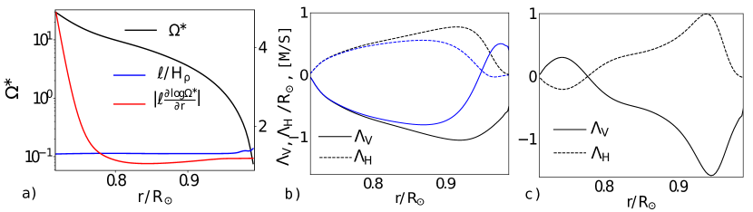
Figure 1: a) Radial profiles of parameters that affect the magnitude and sign of the $\Lambda$-effect: the Coriolis number $\Omega^{*}=2\Omega\tau_{c}$, where $\Omega=2.90\cdot 10^{-6}$ s^-1 is the mean angular velocity (black line), the ratio of the mixing length and the density scale height, $\ell/H_{\rho}$ (blue line), and the ratio of the mixing length and the scale height of the Coriolis number (red); the right vertical axis shows the scale of the last two parameters; b) theoretical profiles of the vertical ($\Lambda_{V}$) and horizontal ($\Lambda_{H}$) components of the $\Lambda$-tensor in the solar convection zone at co-latitude $\theta=45^{\circ}$ for models M1 (blue lines) and M2 (black lines) ; c) the same as b) but for model M3.

For accurate description of the angular momentum transfer, it is important to take into account the effect of the radial profile of the Coriolis number, $\Omega^{*}$, on the $\Lambda$ effect. To illustrate this, we consider the case of fast rotation, $\Omega^{*}\gg 1$. The nondiffusive flux of angular momentum can be expressed as follows:

$$\Lambda_{r\phi\phi}\overline{U}_{\phi} = \Lambda_{V}\Omega\sin\theta,$$ (9)

$$\Lambda_{V} \approx \nu_{T}\cos^{2}\theta\frac{J_{1}\ell}{H_{\rho}}\left(\frac{\ell}{H_{\rho}}+\ell\frac{\partial\log\Omega^{*}}{\partial r}\right),$$ (10)

$$\Lambda_{\theta\phi\phi}\overline{U}_{\phi} = \Lambda_{H}\Omega\cos\theta,$$ (11)

$$\Lambda_{H} \approx -\nu_{T}\sin^{2}\theta\frac{J_{1}\ell}{H_{\rho}}\left(\frac{\ell}{H_{\rho}}+\ell\frac{\partial\log\Omega^{*}}{\partial r}\right),$$ (12)

where $J_{1}=-{\displaystyle\frac{\pi}{4\Omega^{*}},}$ and and $\Lambda_{V}$, $\Lambda_{H}$ are the vertical and horizontal components of the $\Lambda$ effect. We reproduce the original results of Kitchatinov & Rüdiger (1993) if the contribution of the Coriolis number gradient, ${\displaystyle\frac{\partial\log\Omega^{*}}{\partial r}}$, is neglected. We would like to stress that the dependence of the $\Lambda$ effect coefficients on the Coriolis number is included in models M1 and M2. Those models disregard the effect of the spatial derivatives of the $\Omega^{*}$ which seems to be important near the bottom of the convection zone.

However, because the convective overturn time, $\tau_{c}$, in stellar convection zones changes with depth, the radial gradient of the Coriolis number, $\Omega^{*}=2\Omega\tau_{c}$, can be essential for the amplitude and direction of the $\Lambda$ effect. The $\tau_{c}$-profile can be obtained from results of the MESA code using the standard mixing-length approximation, $\tau_{c}=\ell/\mathrm{u}^{\prime}$. Note that with the use of the mixing-length theory for the solar interior model, this formula is equivalent to another expression (see Kippenhahn & Weigert, 1994):

$$\tau_{c}=\left(\frac{4c_{p}\overline{\rho}\ell^{2}\overline{T}}{g\delta F_{con}}\right)^{1/3},$$ (13)

where $F_{con}$ is the amount of heat flux transported by convection, and $\delta=-{\displaystyle\left(\frac{\partial\log\overline{\rho}}{\partial\log\overline{T}}\right)_{P}}$ ($\delta=1$ for an ideal mono-atomic gas). The profile of the Coriolis number calculated from the solar interior model is shown in Figure 1a. It is seen that parameter $|\ell{\displaystyle\frac{\partial\log\Omega^{*}}{\partial r}}|$ is greater than unity in the lower part of the convection zone, and thus it should be taken into account.

Below, we consider results for the mean-field hydrodynamic models of the solar differential rotation based on three models of the $\Lambda$ effect, listed in Table 1. We would like to stress that the dependence of the $\Lambda$ effect coefficients on the Coriolis number is included in models M1 and M2, but these models disregard the radial derivative of the $\Omega^{*}$. Note that models M1 and M2 differ only in the parameter of anisotropy, which is $a=0$ in M1 and $a=2$ in M2. Model M3 includes both the radial derivative of $\Omega^{*}$ and the convective anisotropy.

Figures 1(b) and (c) show the theoretical profiles of components of the $\Lambda$-tensor in the solar convection zone. The impact of the convective velocity anisotropy is illustrated for the anisotropy parameter $a={\displaystyle\frac{\overline{{u_{h}^{2}}}-2\overline{{u_{r}^{2}}}}{\overline{{u_{r}^{2}}}}=}2$, where ${u_{h}}$ and ${u_{r}}$ are the horizontal and vertical RMS velocities. With this parameter value, the radial nondiffusive transport of the angular momentum at the top of the convection zone is negative (model M2). This allows us to model the subsurface shear layer. The contribution of the ${\displaystyle\frac{\partial\log\Omega^{*}}{\partial r}}$ term, included in model M3, also changes the $\Lambda$-effect components. These changes are of two kinds. Firstly, we see that the magnitude of the $\Lambda$-tensor is reduced in the middle of convection zone. Secondly, the vertical and horizontal components of the tensor both change their sign near the bottom of the convection zone, at $r\simeq 0.78~{}R_{\odot}$.

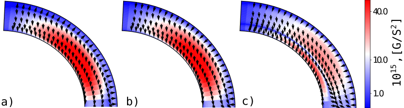
Figure 2: Directions and amplitude of the angular momentum flux due to the $\Lambda$ effect (with the vector components given by Eqs (9) and (11)) in three models: a) M1; b) M2; c) M3, listed in Table 1.

Figure 2 shows the direction of the angular momentum flux by the $\Lambda$ effect for the three models. In all of these cases, the direction of the nondiffusive angular momentum transport is predominantly along the axis of rotation from higher to lower latitudes in the main part of the convection zone. Model M1 shows the outward transport by the $\Lambda$ effect in the upper part of the convection zone. Figure 2b (model M2) illustrates that including effects of the convective velocity anisotropy results in the inward angular momentum transport at the top of the convection zone. This effect was suggested by Kitchatinov (2004). Taking into account contributions of the Coriolis number gradients in the $\Lambda$ effect, we get the inversion of the angular momentum transport of direction near the base of the convection zone (Fig. 1c). In the upper part of the convection zone the pattern shown in Figure 2c is in qualitative agreement with Bekki & Yokoyama (2017) (hereafter, BY17). Near the bottom of the convection zone both, the radial and the horizontal components of the $\Lambda$-effect, change sign. This is different from the model of BY17, who employed an approximate fit of the $\Lambda$-effect profile to satisfy the gyroscopic pumping equation. For convenience, we briefly review this concept. For details and applications, please consult the paper by Miesch & Hindman (2011). Let us introduce the mean specific angular momentum, $\mathcal{L}=r^{2}\sin^{2}\theta\Omega$. Helioseismology tells that, in the solar convection zone, $\mathcal{L}$ is constant on cylinders increasing outward from the rotational axis. For the mean stationary stage, the equation of the angular momentum balance can be approximated as follows:

$$\overline{\rho}\mathbf{\overline{U}_{\zeta}^{m}\nabla_{\zeta}\mathcal{L}} \approx -\boldsymbol{\nabla\cdot}\left(r\sin\theta\hat{\mathbf{T}}_{\phi}\right)$$ (14)

where $\zeta=r\sin\theta$ and we take into account cylinder-like distribution of $\mathcal{L}$. Note, that $\nabla_{\zeta}\mathcal{L}>0$. The double-cell meridional circulation like that found by Zhao et al. (2014) gives the negative $\mathbf{\overline{U}}_{\zeta}^{m}$ at the bottom, positive in the middle, and negative at the top of the convection zone. Then, the LHS of Eq(14) gets the same signs. Therefore, Eq(14) can be satisfied for a radially converging vector field $\hat{\mathbf{T}}_{\phi}$. The pattern demonstrated in Figure 2c satisfies this condition as well as the $\Lambda$-effect model introduced by BY17 (see Fig. 1 in their paper). As it is seen in Figure 2 that for the case of the moderate and fast rotation regimes, $\Omega^{*}>1$, the mean-field theory predicts a nearly cylinder-like distribution of the angular momentum fluxes produced by the $\Lambda$-effect in the rotating stratified convective media. We note that effects of the convective velocity anisotropy are strongly quenched with the increase of the Coriolis number (Kitchatinov et al., 1994; Kitchatinov, 2004).

3 Results

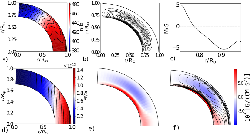
Figure 3: Properties of large-scale flows in model M1 (no inversion of the $\Lambda$- effect sign and $a=0$): a) the distribution of the rotation rate, $\Omega\left(r,\theta\right)/2\pi$, in the solar convection zone; the isolines are plotted in the range of 385-480 nHz nHz with interval of $\approx 7$nHz b) streamlines of the meridional circulation; c) the radial profile of the meridional velocity component at $\theta=45^{\circ}$; d) distribution of the specific angular momentum, $=r^{2}\sin^{2}\theta\Omega$; e) the angular momentum advected by the meridional flow, i.e., $\overline{\rho}\left(\mathbf{\overline{U}}^{m}\cdot\boldsymbol{\nabla}\right)\mathcal{L}$; f) the total torque of the turbulent stresses, $-\nabla\cdot(r\sin\theta\hat{\mathbf{T}}_{\phi})$ (background color) and the torque component from the $\Lambda$-effect (contours), i.e., $-\nabla\cdot(r\sin\theta\hat{\mathbf{T}}_{\phi}^{\left(\Lambda\right)})$, (see, Eqs(3,4) ); both are displayed in the same interval as shown by the color bar.

Numerical solutions of Eq. (1)-(5) for the three models of Table 1 are shown in Figures 3-5. Figures 3(a)-(c) show profiles of the angular velocity, streamlines of the meridional circulation and the radial profile of the meridional flow velocity at $\theta=45^{\circ}$ for model M1. The amplitude of the poleward meridional flow velocity is of $\sim 5$ m s^-1 at the surface, and the same velocity is found near the bottom. These results are similar to the models of Küker et al. (1993) and Kitchatinov et al. (1994). Some differences with their models are likely due to the different models of the solar interior and the $\tau_{c}$ profile. Model M1 shows a positive gradient of the angular velocity near the surface, as found in the above cited papers, as well. However, this is not consistent with results of helioseismology inversions (Schou et al., 1998; Howe et al., 2011). Figures 3d shows distribution of the specific angular momentum. It has a cylinder-like profile (cf. Miesch & Hindman, 2011). Contrary to the observations it shows the poleward deviations of the isolines in the near-surface layer. Figures 3 e and f , show the angular momentum advected by the meridional flow, i.e., $\overline{\rho}\left(\mathbf{\overline{U}}^{m}\cdot\boldsymbol{\nabla}\right)\mathcal{L}$, and the rotational forces of the $\Lambda$-effect, i.e., $-\nabla\cdot(r\sin\theta\hat{\mathbf{T}}_{\phi}^{\left(\Lambda\right)})$, and the same for the total turbulent stress, $-\nabla\cdot(r\sin\theta\hat{\mathbf{T}}_{\phi}^{\left(\Lambda\right)})$, (see, Eqs(3,4). We see that the effect of the meridional flow is in balance with the turbulent stresses. Contrary to results of BY17 signs of the torque from the $\Lambda$-effect are not fully balanced with the meridional circulation. This means that the effect of the diffusive part of the angular momentum is also important. Our models take into account the anisotropic eddy viscosity. Its importance for the mean-field models of the solar differential rotations was addressed previously by Küker et al. (1993) and Kitchatinov et al. (1994). The mean direction of the turbulent angular momentum flux corresponds to the direction of the nondiffusive flux driven by the $\Lambda$- effect (see, Fig.2a). Note that the amplitude of the near-surface meridional circulation is suppressed. Moreover, the model of Kitchatinov et al. (1994) has a weak clockwise circulation cell near the surface. Their model, as well as model M1, has positive radial shear at the surface. In both cases, it results from the $\Lambda$- effect profile which corresponds to the outward angular momentum flux.

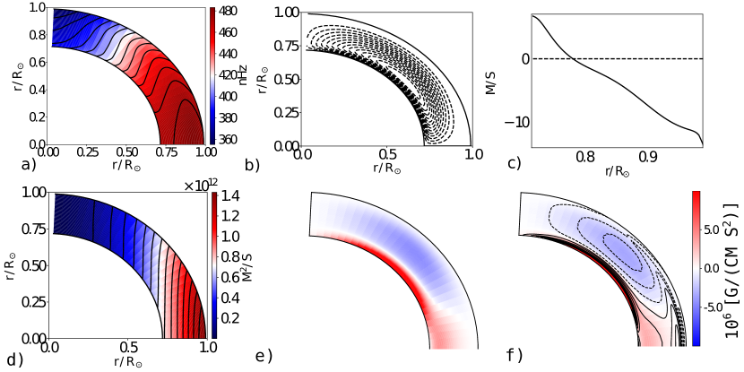
Figure 4: The same as Figure 3 for model M2.

Taking into account the convective velocity anisotropy in the $\Lambda$-effect formulation, Kitchatinov (2004) and Kitchatinov & Rüdiger (2005) showed that the mean-field model can approximately reproduce the subsurface rotational shear. Figure 4 shows results for model M2. The results are similar to those in Kitchatinov (2004). The amplitude of the surface poleward meridional flow velocity is about 10 m/s. Similarly to the results of Kitchatinov (2004), the stagnation point of the meridional circulation streamline is located near the bottom of the convection zone. Similarly to the model M1, the model M2 shows a balance between distributions of the angular momentum transport by the meridional circulation and by the turbulent stresses. This is illustrated by Figures 4e and f.

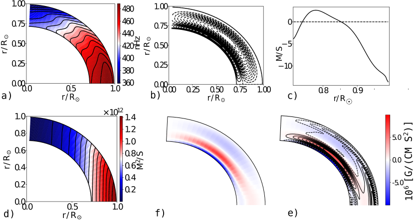
Figure 5: The same as Figure 3 for model M3.

The results for our complete model M3 (with the sign inversion of the $\Lambda$- effect and convective anisotropy) are presented in Fig. 5. The model shows the double-cell circulation pattern with the upper stagnation point located at $r=0.85R_{\odot}$. Observational results of Hathaway (2012) and Zhao et al. (2013) show it at about $0.92R_{\odot}$, and Böning et al. (2017) found at $0.9R_{\odot}$. The amplitude of the surface poleward flow is about 10 m s^-1. It is likely that our model underestimates the photospheric magnitude of the meridional flow because the top of the integration domain is located below the photospheric level. The angular velocity profile shows a strong subsurface shear, as well as an increased radial gradient at the bottom.

Compared to models M1 and M2, model M3 shows a weak poleward turbulent angular momentum flux near the bottom of the convection zone (see Figure 2c). It results from the $\Lambda$-effect profile. The distribution of the angular momentum density advected by the meridional flow, $\overline{\rho}\left(\mathbf{\overline{U}}^{m}\cdot\boldsymbol{\nabla}\right)\mathcal{L}$, (Fig. 5e) is very similar to results of BY17. Excluding some difference in the near equatorial regions, both the model of BY17 and our model M3 have similar distributions of the torque produced by the $\Lambda$-effect, in particular, the negative torque at the bottom and at the top of the convection zone. Model M3 shows the positive torque near the equator with maximum below the subsurface shear. This is different from BY17, and is likely due to the more complicated structure of the $\Lambda$-effect in our model. At the bottom boundary, the negative $\Lambda$-effect results in the positive radial shear of the angular velocity. In high-latitude regions, the existence of such feature disagrees with the helioseismology inversions of Howe et al. (2011). It is likely that the issue cannot be consistently resolved without considering dynamics of the solar tachocline. This problem is outside the scope of this paper.

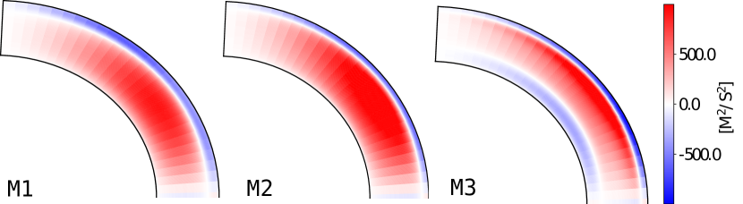
Figure 6: Distributions of $\left\langle{u^{\prime}_{\theta}u^{\prime}_{\phi}}\right\rangle$ in models M1, M2 and M3.

Figure 6 shows the correlation of turbulent velocities, $\left\langle{u^{\prime}_{\theta}u^{\prime}_{\phi}}\right\rangle$, for the all three models. It is positive in the bulk of the convection zone except the near-surface layer. Models M1 and M2 agree with earlier conclusions of Küker et al. (1993). In model M3, this correlation is negative near the bottom of the convection zone. The maximum of $\left\langle{u^{\prime}_{\theta}u^{\prime}_{\phi}}\right\rangle$ is about $10^{3}~{}$m²s^-2. This is in agreement by an order of magnitude with the model of BY17. In model M3, the correlation $\left\langle{u^{\prime}_{\theta}u^{\prime}_{\phi}}\right\rangle$ has a peak near the bottom boundary of the subsurface shear layer. We compare this result with observations in the next section.

Our results suggest that the model of the meridional circulation is sensitive to the choice of the radial Coriolis number profile in the convection zone. In particular, we found that there is no sign inversion of the $\Lambda$-effect for the profile of Stix (2002),

$$\Omega^{*}=\Omega_{0}^{*}\left(\frac{x}{x_{0}}\right)^{7/6}\left(\frac{1-x}{1-x_{0}}\right)^{3/2},$$

where $x=r/R_{\odot}$, and $\Omega_{0}^{*}$ is the Corioils number at $x_{0}=0.8$ (e.g., $\Omega_{0}^{*}\equiv 3$). Using this profile and taking into account the inhomogeneity of the Coriolis number we get no inversion of the $\Lambda$-effect. Results of that model are very similar to our model M2.

4 Discussion and conclusions

In this paper, we have presented a new model of the angular momentum transport. The model naturally explains the double-cell meridional circulation structure. We confirm the conclusions of Bekki & Yokoyama (2017) that the sign inversion of the radial part of the $\Lambda$-effect in the solar convection zone results in the double-cell meridional circulation.

Our model demonstrated that the double-cell meridional circulation pattern can result from the radial gradient of the Coriolis number, which leads to the sign inversion of the nondissipative angular momentum flux (the so-called $\Lambda$-effect) in the low part of the solar convection zone. In our model, both the radial and horizontal components of the $\Lambda$-effect change sign in the lower part of the convection zone. The vector field of the nondiffusive angular momentum transport in our most complete model M3 converges in the middle of the convection zone. Therefore, the resulting profile of the $\Lambda$-effect is consistent with the gyroscopic pumping arguments. Despite the fact that in this paper the viscous part of the gyroscopic pumping equation is substantially different from the simplified version of Bekki & Yokoyama (2017) the resulting distribution of the $\Lambda$-effect in the solar convection zone is qualitatively similar.

We conclude that the knowledge of the convective turnover time distribution is very important for robustness of the mean-field model prediction of the large-scale flow structure inside the solar convection zone. Moreover, the mixing-length theory’s estimation of the turbulent parameters, like the characteristic time-scale, $\tau_{c}$; the mixing length, $\ell$; and the convective velocity RMS ${u^{\prime}}$ may not be sufficiently accurate at the convective zone boundaries because of overshooting and anisotropy of convection.

Pipin & Kosovichev (2016) studied the robustness of the meridional circulation structure with respect to variations of the latitudinal profiles of the radial $\Lambda$-effect. They found that the small increase of the radial $\Lambda$-effect toward the equator can result to the multi-cell meridional circulation structure as well. The obtained pattern of the meridional circulation is different to results of Zhao et al. (2014). We can conclude that the variations of the latitudinal profiles of the radial $\Lambda$-effect are less important to reproduce the results of helioseismology. To understand the nature of the multi-cell meridional circulation in the stellar convection zone the further theoretical progress in the theory of the $\Lambda$-effect is needed.

The original theoretical formulation was obtained by Kitchatinov & Rüdiger (1993) using the second-order correlation approximation (SOCA, Krause & Rädler 1980) for the forced isothermal turbulence rather than for the stellar turbulent convection. The numerical simulations of Käpylä et al. (2011) suggest that in general case the SOCA can be valid only by an order of magnitude. Another need for the future development follows from direct numerical simulations. They often show multiple meridional circulation cells, see, e.g., Guerrero et al. (2016) or Warnecke et al. (2018). These results are difficult to explain within our model. In our paper, we discussed components of the $\Lambda$-effect, which contribute to the generation of the azimuthal large-scale flow. In addition to them, there is a theoretical possibility for the $\Lambda$-effect components which generate the meridional circulation. This effect results from the nondissipative part of the off-diagonal turbulent stresses: $\hat{T}_{r\theta}=\left\langle{u^{\prime}_{\theta}u^{\prime}_{r}}\right\rangle-{\displaystyle\frac{1}{4\pi\overline{\rho}}}\left\langle{b^{\prime}_{\theta}b^{\prime}_{r}}\right\rangle$, where $\boldsymbol{{u}}^{\prime}$ and $\boldsymbol{{b}}^{\prime}$ are the fluctuating velocity and magnetic field. The origin of this effect can be tightly related to inhomogeneities of the kinetic and magnetic helicities of turbulent flows (Yokoi & Brandenburg, 2016). It is interesting that the so-called “anisotropic kinetic alpha - effect” or the “AKA-effect” (Frisch et al., 1987; Pipin et al., 1996; Brandenburg & Rekowski, 2001) also results in the nondissipative part of the $\hat{T}_{r\theta}$ (as well as the azimuthal components of $\mathbf{\hat{T}}$). Therefore, the theory of the $\Lambda$-effect, which is employed in our paper is rather incomplete.

The model correlation $\left\langle{u^{\prime}_{\theta}u^{\prime}_{\phi}}\right\rangle$ can be compared with motions of sunspots (Sudar et al., 2017) and the large-scale magnetic fields (Latushko, 1993). Both of these measurements show the positive correlation in the northern hemisphere of the Sun. The sign of $\left\langle{u^{\prime}_{\theta}u^{\prime}_{\phi}}\right\rangle$ is the main reason for the solar-like differential rotation with the equator rotating faster than the poles (Rüdiger, 1989). Model M3 has the positive $\left\langle{u^{\prime}_{\theta}u^{\prime}_{\phi}}\right\rangle$ in the middle of the convection zone of the northern hemisphere of the Sun. By comparing the model results with the measurements of $\left\langle{u^{\prime}_{\theta}u^{\prime}_{\phi}}\right\rangle$ from sunspot motions and the large-scale magnetic field tracers, we can conclude that these features are likely rooted just below the subsurface shear layer. Model M3 excludes positive values of $\left\langle{u^{\prime}_{\theta}u^{\prime}_{\phi}}\right\rangle$ for the magnetic field anchored at the bottom of the convection zone. These conclusions agree with results of Benevolenskaya et al. (1999) on rotation of newly emerged active regions.

In summary, the double-cell meridional circulation on the Sun is naturally explained in our model because of a concurrent effect of the density stratification and variations of the Coriolis force acting on the cyclonic convection. The key point is that the variation of the convective turnover time with depth result in inversion of the sign of the non-dissipative turbulent stresses (the $\Lambda$-effect) in the lower part of the convection zone. However, the properties of the turbulent angular momentum transport employed in this paper using the mean-field hydrodynamics approach require further studies with the help of observations and numerical simulations.

Acknowledgments. Valery V. Pipin thanks the grant of Visiting Scholar Program supported by the Research Coordination Committee, National Astronomical Observatory of Japan (NAOJ). Also, a support from of RFBR grants 16-52-50077 and 17-52-53203, and support of project II.16.3.1 of ISTP SB RAS are greatly acknowledged. Alexander Kosovichev thanks a support of NASA’s grants NNX 14AB70G and NNX 17AE76A

5 Appendix

5.1 The turbulent stress tensor

Expression of the turbulent stress tensor results from the mean-field hydrodynamics theory (see, Kitchatinov et al. 1994; Kitchatinov 2004) as follows:

$${\hat{T}_{ij}=\overline{\rho}\left\langle u_{i}u_{j}\right\rangle,}$$ (15)

where ${u}$ is fluctuating velocity. Application the mean-field hydrodynamic framework leads to the Taylor expansion given by Eq(4). The viscous part of the azimuthal components of the stress tensor is determined following Kitchatinov et al. 1994 in the following form:

$${T_{r\phi}^{(\nu)}} {=} -{\overline{\rho}\nu_{T}\left\{\Phi_{\perp}+\left(\Phi_{\|}-\Phi_{\perp}\right)\mu^{2}\right\}r\frac{\partial\sin\theta\Omega}{\partial r}}$$

$$- {\overline{\rho}\nu_{T}\sin\theta\left(\Phi_{\|}-\Phi_{\perp}\right)\left(1-\mu^{2}\right)\frac{\partial\Omega}{\partial\mu}}$$

$${T_{\theta\phi}^{(\nu)}} {=} {\overline{\rho}\nu_{T}\sin^{2}\theta\left\{\Phi_{\perp}+\left(\Phi_{\|}-\Phi_{\perp}\right)\sin^{2}\theta\right\}\frac{\partial\Omega}{\partial\mu}}$$

$$+ {\overline{\rho}\nu_{T}\left(\Phi_{\|}-\Phi_{\perp}\right)\mu\sin^{2}\theta r\frac{\partial\Omega}{\partial r}},$$

where the eddy viscosity, $\nu_{T}$, is determined from the mixing-length theory assuming the turbulent Prandl number ${Pr}_{T}={\displaystyle\frac{3}{4}}$:

$$\nu_{T}=\frac{3\ell^{2}}{8}\sqrt{-\frac{g}{2c_{p}}\frac{\partial\overline{{s}}}{\partial r}}.$$

The viscosity quenching functions, $\Phi_{\perp}$ and $\Phi_{\parallel}$, depend nonlinearly on the Coriolis number, $\Omega^{*}=2\Omega\tau_{c}$ and they are determined by Kitchatinov et al. (1994).

The nondiffusive flux of angular momentum can be expressed as follows (Rüdiger, 1989):

$$\Lambda_{r\phi\phi}\overline{U}_{\phi} = r\Lambda_{V}\Omega\sin\theta,$$

$$\Lambda_{V} = \nu_{T}\left(V^{(0)}+\sin^{2}\theta V^{(1)}\right),$$ (18)

$$\Lambda_{\theta\phi\phi}\overline{U}_{\phi} = r\Lambda_{H}\Omega\cos\theta,$$

$$\Lambda_{H} = \nu_{T}\sin^{2}\theta H^{(1)}$$ (19)

The basic contributions to the $\Lambda$-effect are due to the density stratification and the Coriolis force. Kitchatinov & Rüdiger (1993) found the following expression for the $\Lambda$-tensor coefficients:

$$V^{(0,\rho)} = \frac{r}{\rho^{2}}\frac{\partial}{\partial r}\left(\frac{1}{r}\frac{\partial}{\partial r}\tau^{2}\left\langle\boldsymbol{u}^{\prime 2}\right\rangle\rho^{2}\left(I_{1}-I_{2}\right)\right)$$

$$+ \tau^{2}\left\langle\boldsymbol{u}^{\prime 2}\right\rangle\rho^{2}\left(I_{3}-I_{4}\right)r\frac{\partial}{\partial r}\frac{1}{r\rho}\frac{\partial\rho}{\partial r}$$

$$+ \frac{1}{\rho^{3}}\frac{\partial\rho}{\partial r}\frac{\partial}{\partial r}\tau^{2}\left\langle\boldsymbol{u}^{\prime 2}\right\rangle\rho^{2}\left(I_{5}-I_{6}\right),$$

$$V^{(1,\rho)} = \frac{r}{\rho^{2}}\frac{\partial}{\partial r}\left(\frac{1}{r}\frac{\partial}{\partial r}\tau^{2}\left\langle\boldsymbol{u}^{\prime 2}\right\rangle\rho^{2}I_{2}\right)$$

$$+ \tau^{2}\left\langle\boldsymbol{u}^{\prime 2}\right\rangle\rho^{2}I_{4}r\frac{\partial}{\partial r}\frac{1}{r\rho}\frac{\partial\rho}{\partial r}$$

$$+ \frac{1}{\rho^{3}}\frac{\partial\rho}{\partial r}\frac{\partial}{\partial r}\tau^{2}\left\langle\boldsymbol{u}^{\prime 2}\right\rangle\rho^{2}\left(I_{5}-I_{6}\right),$$

where $I_{n}$ are functions of the Coriolis number and $H^{(1,\rho)}=-V^{(1,\rho)}$. If we neglect the contributions of all inhomogeneities except the density stratification and variations of the Coriolis number in functions $I_{n}$ we get the following results:

$$V^{(0,\rho)} = \left(\frac{\ell}{H_{\rho}}\right)^{2}\left(J_{0}+J_{1}\right)-\frac{\ell^{2}}{H_{\rho}}\frac{\partial}{\partial r}\left\{\left(J_{0}+J_{1}\right)-I_{5}+I_{6}\right\}+\ell^{2}\frac{\partial^{2}}{\partial r^{2}}\left(I_{1}-I_{2}\right),$$ (22)

$$V^{(1,\rho)} = -\left(\frac{\ell}{H_{\rho}}\right)^{2}J_{1}+\frac{\ell^{2}}{H_{\rho}}\frac{\partial}{\partial r}\left\{J_{1}+I_{6}\right\}+\ell^{2}\frac{\partial^{2}}{\partial r^{2}}I_{2},$$ (23)

where, $H_{\rho}=-{\displaystyle\left(\frac{\partial\log\bar{\rho}}{\partial r}\right)^{-1}}$ , $J_{0}=4I_{1}+2I_{5}$ and $J_{1}=-4I_{2}-2I_{6}$ are defined in the above cited paper. Functions $I_{n}$ have the following form (also, see, Kitchatinov & Rüdiger 1993):

$$I_{1} = \frac{1}{4\Omega^{*4}}\left(\frac{6+5\Omega^{*2}}{1+\Omega^{*2}}-\left(6+\Omega^{*2}\right)\frac{\arctan\Omega^{*}}{\Omega^{*}}\right),$$

$$I_{2} = \frac{1}{8\Omega^{*4}}\Bigl{(}60+\Omega^{*2}-\frac{6\Omega^{*2}}{1+\Omega^{*2}}$$

$$+ \left(\Omega^{*4}-15\Omega^{*2}-60\right)\frac{\arctan\Omega^{*}}{\Omega^{*}}\Bigr{)},$$

$$I_{3} = \frac{1}{2\Omega^{*4}}\left(-3+\frac{\Omega^{*2}}{1+\Omega^{*2}}+3\frac{\arctan\Omega^{*}}{\Omega^{*}}\right),$$

$$I_{4} = \frac{1}{2\Omega^{*4}}\left(-15+\frac{2\Omega^{*2}}{1+\Omega^{*2}}+\left(15+3\Omega^{*2}\right)\frac{\arctan\Omega^{*}}{\Omega^{*}}\right),$$

$$I_{5} = \frac{1}{2\Omega^{*4}}\left(-3+\left(\Omega^{*2}+3\right)\frac{\arctan\Omega^{*}}{\Omega^{*}}\right),\,I_{6}=\frac{1}{2}I_{4}.$$

Using the mixing-length approximation for the adiabatic distribution of the thermodynamic parameters we define the mixing-length parameter as follows: ${\displaystyle\frac{\ell}{H_{\rho}}\equiv\frac{\alpha_{MLT}}{\gamma}}$. As was noted by Kitchatinov & Rüdiger 1993 in case of $\Omega^{*}\ll 1$ we have: ${\displaystyle I_{1}=\frac{1}{30}}$, ${\displaystyle I_{3}=-\frac{1}{5}}$, ${\displaystyle I_{5}=\frac{1}{15}}$, and $I_{2,4,6}=0$. Therefore the derivatives of $I_{n}$ and $J_{0,1}$ in Eq(22) and Eq(23) can be neglected.

For case of fast rotation, it is found $I_{2}={\displaystyle\frac{\pi}{16\Omega^{*}},}$ $J_{1}={\displaystyle-\frac{\pi}{4\Omega^{*}},}$ and others functions are of $O\left(\Omega^{*-3}\right)$. Then for $V^{(0,\rho)}$ from Eq(22) we have

$$V^{(0,\rho)} \approx \frac{\ell}{H_{\rho}}J_{1}\left(\frac{\ell}{H_{\rho}}+\ell\frac{\partial\log\Omega^{*}}{\partial r}\right),$$ (24)

$$V^{(1,\rho)} \approx -\frac{\ell}{H_{\rho}}J_{1}\left(\frac{\ell}{H_{\rho}}+\ell\frac{\partial\log\Omega^{*}}{\partial r}\right)$$ (25)

where the first term is positive , and the second term is negative (as the $\Omega^{*}$ decreased toward surface) . The first term dominate in the upper part of the convection zone but the second term increases steeply toward the bottom, and overcome the first one (Fig. 1a) and the density height scale varies slowly. We conclude that it is important to keep the second contributions in Eq(22) and Eq(23).

In the final expressions of the $\Lambda$-effect we take into account anisotropy of convective velocities (see, Kitchatinov 2004). Therefore, the final coefficients of the $\Lambda$-tensor are:

$$V^{(0)} = \Bigl{[}\left(\frac{\alpha_{MLT}}{\gamma}\right)^{2}\left\{J_{0}+\!J_{1}+\!a\left(I_{0}+\!I_{1}\right)\right\}$$

$$- \Bigl{(}\frac{\alpha_{MLT}\ell}{\gamma}\frac{\partial}{\partial r}\left\{\left(J_{0}+J_{1}\right)-I_{5}+I_{6}\right\}+\ell^{2}\frac{\partial^{2}}{\partial r^{2}}\left(I_{1}-I_{2}\right)\Bigr{]},$$

$$V^{(1)} = -\left\{\left(\frac{\alpha_{MLT}}{\gamma}\right)^{2}\left(J_{1}+aI_{1}\right)-\frac{\alpha_{MLT}\ell}{\gamma}\frac{\partial}{\partial r}\left(J_{1}+I_{6}\right)-\ell^{2}\frac{\partial^{2}}{\partial r^{2}}I_{2}\right\},$$ (27)

and ${H^{(1)}=-V^{(1)}}$. We employ the parameter of the turbulence anisotropy $a={\displaystyle\frac{\overline{{u_{h}^{2}}}-2\overline{{u_{r}^{2}}}}{\overline{{u_{r}^{2}}}}=}2$, where ${u_{h}}$ and ${u_{r}}$ are the horizontal and vertical RMS velocities (Kitchatinov, 2004).

The first RHS term of Eq.(5) describes dissipation of the mean vorticity, $\omega$. Similarly to Rempel (2005) we approximate it as follows,

$$-{\left[\boldsymbol{\nabla}\times\frac{1}{\overline{\rho}}\boldsymbol{\nabla\cdot}\overline{\rho}\hat{\mathbf{T}}\right]_{\phi}\approx 2\nu_{T}\phi_{1}\left(\Omega^{*}\right)\nabla^{2}\omega,}$$ (28)

where the rotational quenching function $\phi_{1}$ is given by Kitchatinov et al. (1994). We have tried to apply a more general formalism including all components of the eddy-viscosity tensor for rotating turbulence provided by Kitchatinov et al. (1994), and obtained results that are similar to the approximation given by Eq(28).

References

- Bekki & Yokoyama (2017) Bekki, Y., & Yokoyama, T. 2017, ApJ, 835, 9
- Benevolenskaya et al. (1999) Benevolenskaya, E. E., Hoeksema, J. T., Kosovichev, A. G., & Scherrer, P. H. 1999, ApJ, 517, L163
- Böning et al. (2017) Böning, V. G. A., Roth, M., Jackiewicz, J., & Kholikov, S. 2017, 2017, ApJ, 845, 2
- Brandenburg & Rekowski (2001) Brandenburg, A., & Rekowski, B. V. 2001, A&A, 379, 1153
- Durney (1999) Durney, B. R. 1999, ApJ, 511, 945
- Featherstone & Miesch (2015) Featherstone, N. A., & Miesch, M. S. 2015, ApJ, 804, 67
- Frisch et al. (1987) Frisch, U., She, Z. S., & Sulem, P. L. 1987, Physica D Nonlinear Phenomena, 28, 382
- Gastine et al. (2013) Gastine, T., Wicht, J., & Aurnou, J. M. 2013, Icarus, 225, 156
- Guerrero et al. (2016) Guerrero, G., Smolarkiewicz, P. K., de Gouveia Dal Pino, E. M., Kosovichev, A. G., & Mansour, N. N. 2016, ApJ, 819, 104
- Guerrero et al. (2013) Guerrero, G., Smolarkiewicz, P. K., Kosovichev, A. G., & Mansour, N. N. 2013, ApJ, 779, 176
- Hathaway (2012) Hathaway, D. H. 2012, ApJ, 760, 84
- Hotta et al. (2015) Hotta, H., Rempel, M., & Yokoyama, T. 2015, in Astronomical Society of the Pacific Conference Series, Vol. 498, Numerical Modeling of Space Plasma Flows ASTRONUM-2014, ed. N. V. Pogorelov, E. Audit, & G. P. Zank, 154
- Howe et al. (2011) Howe, R., Larson, T. P., Schou, J., Hill, F., Komm, R., Christensen-Dalsgaard, J., & Thompson, M. J. 2011, Journal of Physics Conference Series, 271, 012061
- Käpylä et al. (2014) Käpylä, P. J., Käpylä, M. J., & Brandenburg, A. 2014, A&A, 570, A43
- Käpylä et al. (2011) Käpylä, P. J., Mantere, M. J., Guerrero, G., Brandenburg, A., & Chatterjee, P. 2011, A&A, 531, A162
- Kholikov et al. (2014) Kholikov, S., Serebryanskiy, A., & Jackiewicz, J. 2014, ApJ, 784, 145
- Kippenhahn & Weigert (1994) Kippenhahn, R., & Weigert, A. 1994, Stellar Structure and Evolution, 192
- Kitchatinov (2004) Kitchatinov, L. L. 2004, Astronomy Reports, 48, 153
- Kitchatinov et al. (1994) Kitchatinov, L. L., Pipin, V. V., & Rüdiger, G. 1994, Astronomische Nachrichten, 315, 157
- Kitchatinov & Rüdiger (1993) Kitchatinov, L. L., & Rüdiger, G. 1993, A&A, 276, 96
- Kitchatinov & Rüdiger (2005) Kitchatinov, L. L., & Rüdiger, G. 2005, Astronomische Nachrichten, 326, 379
- Krause & Rädler (1980) Krause, F., & Rädler, K.-H. 1980, Mean-Field Magnetohydrodynamics and Dynamo Theory (Berlin: Akademie-Verlag), 271
- Küker et al. (1993) Küker, M., Rüdiger, G., & Kitchatinov, L. L. 1993, A&A, 279, L1
- Latushko (1993) Latushko, S. 1993, Sol. Phys., 146, 401
- Miesch & Hindman (2011) Miesch, M. S., & Hindman, B. W. 2011, ApJ, 743, 79
- Paxton et al. (2011) Paxton, B., Bildsten, L., Dotter, A., Herwig, F., Lesaffre, P., & Timmes, F. 2011, ApJS, 192, 3
- Paxton et al. (2013) Paxton, B., et al. 2013, ApJS, 208, 4
- Pipin & Kosovichev (2016) Pipin, V. V., & Kosovichev, A. G. 2016, Advances in Space Research, 58, 1490
- Pipin et al. (1996) Pipin, V. V., Rüdiger, G., & Kitchatinov, L. L. 1996, Geophysical and Astrophysical Fluid Dynamics, 83, 119
- Rajaguru & Antia (2015) Rajaguru, S. P., & Antia, H. M. 2015, ApJ, 813, 114
- Rempel (2005) Rempel, M. 2005, ApJ, 622, 1320
- Rüdiger (1989) Rüdiger, G. 1989, Differential rotation and stellar convection. Sun and the solar stars
- Schad et al. (2013) Schad, A., Timmer, J., & Roth, M. 2013, ApJ, 778, L38
- Schou et al. (1998) Schou, J., et al. 1998, Astrophys. J., 505, 390
- Stix (2002) Stix, M. 2002, The sun: an introduction, 2nd edn. (Berlin : Springer), 521
- Sudar et al. (2017) Sudar, D., Brajša, R., Skokić, I., Poljančić Beljan, I., & Wöhl, H. 2017, Sol. Phys., 292, 86
- Warnecke et al. (2018) Warnecke, J., Rheinhardt, M., Tuomisto, S., Käpylä, P. J., Käpylä, M. J., & Brandenburg, A. 2018, 2018, A&A, 609, A51
- Yokoi & Brandenburg (2016) Yokoi, N., & Brandenburg, A. 2016, Phys. Rev. E, 93, 033125
- Zhao et al. (2013) Zhao, J., Bogart, R. S., Kosovichev, A. G., Duvall, Jr., T. L., & Hartlep, T. 2013, ApJ, 774, L29
- Zhao et al. (2014) Zhao, J., Kosovichev, A. G., & Bogart, R. S. 2014, ApJ, 789, L7