General formulae for dipole Wilson line correlators with the Color Glass Condensate

Abstract

We present general formulae to compute Wilson line correlators with the Color Glass Condensate described by the McLerran-Venugopalan model. We explicitly construct a complete and non-orthogonal set of color-singlet bases and write matrix elements down, so that the exponential of the matrix leads to the Wilson line correlators. We further develop a systematic perturbative expansion of dipole Wilson line correlators in terms of $1/N_{\mathrm{c}}$ where $N_{\mathrm{c}}$ is the color number. As a phenomenological application we calculate the flow harmonics $v_{n}\{m\}$ in the dipole model and discuss the $N_{\mathrm{c}}$ scaling.

1 Introduction

Quantum Chromodynamics (QCD) has a special property called the asymptotic freedom that implies that the strong coupling constant runs to a smaller value in parton reactions involving harder momentum scales. In this way the perturbative calculation of QCD is a reliable theoretical description in high-energy nuclear physics. In reality, however, a naïve perturbative expansion breaks down for diffractive type reactions in which exchanged momenta are not necessary hard as compared to the collision energy. Then, it is indispensable to make a resummation over large logarithmic enhancement factors which appear kinematically. Such a resummation leads to a picture of increasing parton or gluon density with increasing scattering energy, and, one would anticipate that the parton density would eventually enter a new regime where the effect of parton overlapping is significant. In such a regime of dense partons, QCD is still perturbative in a sense that the running coupling constant $g$ is small, but is highly non-linear due to the gluon amplitude $A^{\mu}$ as large as $\sim 1/g$ [and thus $gA^{\mu}\sim\mathcal{O}(1)$]. This non-linear dynamics is a manifestation of the parton or gluon saturation (see Refs. Mueller:1993rr ; Mueller:1994jq ; Balitsky:1995ub ; Balitsky:2001re ; Kovchegov:1999yj for pioneering extensions including the non-linearity, see also Refs. Gelis:2012ri ; Blaizot:2016qgz for recent reviews).

The virtue of the gluon saturation is that physical observables exhibit universal behavior in terms of scaling variables, from which the saturation momentum, $Q_{\mathrm{s}}$, can be experimentally fixed Stasto:2000er . The theoretical framework in the saturation regime to compute physical observables as functions of $Q_{\mathrm{s}}$ has been well established and known as the Color Glass Condensate (CGC) McLerran:1993ni ; McLerran:1993ka ; McLerran:1994vd . The CGC effective theory is elegantly formulated in the renormalization group language JalilianMarian:1997jx ; JalilianMarian:1997gr ; JalilianMarian:1997dw , in which the soft gluons are given by the classical Yang-Mills fields from the hard parton color source Kovchegov:1996ty whose transverse density is characterized by $Q_{\mathrm{s}}^{2}$. The non-linear quantum evolution equation for the color source distribution is known as the JIMWLK equation named after the authors of the pioneering works JalilianMarian:1997jx ; JalilianMarian:1997gr ; JalilianMarian:1997dw ; Iancu:2000hn ; Ferreiro:2001qy . Although solving the JIMWLK equation demands huge computational resources (see, for example, Ref. Weigert:2000gi for the reformulation using the Langevin equation, and Refs. Rummukainen:2003ns ; Lappi:2015fma for numerical simulations), a Gaussian approximated solution has been derived Iancu:2002aq ; Lappi:2012nh . The simplest CGC model in the Gaussian approximation is commonly called the McLerran-Venugopalan (MV) model, which is often used as an initial input for the JIMWLK evolution, or, this model itself could provide us with a good description of the qualitative features of high-energy QCD processes.

One of the most interested and testable quantities calculated in the CGC framework is the particle production Kovner:2001vi ; Kovchegov:2001sc ; Blaizot:2004wu ; Blaizot:2004wv and correlation Baier:2005dv ; Marquet:2007vb ; Fukushima:2008ya ; Albacete:2010pg ; Kovner:2016jfp , including electromagnetic probes Gelis:2002ki ; Gelis:2002fw ; JalilianMarian:2004er ; Benic:2016yqt ; Benic:2016uku . In the MV model various correlations among gluons and quarks have been discussed, and these predictions are to be compared to the experimental data of jets and hadron correlations. One of the most well known examples is the CGC picture to understand the ridge structure seen in the di-jet or di-hadron correlations in rapidity space Dumitru:2008wn ; Dumitru:2010iy . Thus, it would be a natural extension to apply the CGC-based calculations to account for the collective behavior in small size systems. As the collision energy grows up, small size systems such as the $p$-$A$ (proton-nucleus) and even the $p$-$p$ collisions may look similar to the $A$-$A$ collision, yielding systematic patterns of the flow observables (see Ref. Loizides:2016tew for an experimental overview). The final state interaction might be still responsible for the flow observables, but at the same time, one must also estimate the initial state effect to quantify which of the initial and the final state interactions is more important. Recently, within the dipole model for the particle production the systematics of the higher order flow observables, $v_{n}\{m\}$ (i.e. $n$-th harmonics of the $m$-particle flow) has been quantified in the glasma graph approximation Skokov:2014tka ; Lappi:2015vta and in the full MV model Dusling:2017dqg ; Dusling:2017aot .

Generally, in the CGC model calculations, the most time-consuming part in numerics is the numerical computation of the expectation value of the Wilson lines. In the presence of the CGC background fields corresponding to the saturated soft gluons, one needs to take account of multiple scatterings which amount to the Wilson line in the eikonal approximation. It has been repeatedly discussed how to compute the Wilson line correlators efficiently in separate contexts (see Ref. Shi:2017gcq for a very recent work toward general formulae for the Wilson line correlators, for instance). Therefore, it would be quite useful to establish a prescription to compute the Wilson line correlators with some generality but in a fairly straightforward way. There are several preceding works along these lines from an early attempt in Ref. Fukushima:2007dy to a very recent reformulation in Ref. Dumitru:2017cwt on top of an explicit calculation in Ref. Shi:2017gcq . The purpose of the present work is to translate the powerful method of Ref. Fukushima:2007dy to a more specific physics problem in a more handy form. In particular, the setup in Ref. Fukushima:2007dy was too general and it was not clear how to utilize the formulae for phenomenological applications. In the present work, hence, we focus on the special type of correlation function in terms of the dipole operators in the color fundamental representation, which is the basic building block in the dipole model Kowalski:2006hc . For $n$-point dipole correlations the problem is reduced to the exponentiation of $n!\times n!$ matrices. The calculation of the exponential of the matrix is numerically feasible but it is sometimes insightful to perform the large-$N_{\mathrm{c}}$ expansion, especially to identify the $N_{\mathrm{c}}$ scaling of observables. We emphasize that our formulae take a quite convenient form for the large-$N_{\mathrm{c}}$ expansion and we will demonstrate the expansion explicitly up to the order where the first nonzero flow cumulants appear. We check the validity of the large-$N_{\mathrm{c}}$ formulae by comparing to the exact results known for $n=2$ with $N_{\mathrm{c}}=3$. For $n\geq 4$ we need to be very careful of the correct large-$N_{\mathrm{c}}$ counting and we will argue the subtlety in the numerical analysis.

2 Master formulae

The Wilson line correlators that we calculate in this paper are expressed in analogy to quantum mechanics as follows Fukushima:2007dy :

$$\biggl{\langle}\prod_{i=1}^{n}U({\boldsymbol{x}_{\perp}}_{i})_{\beta_{i}\alpha_{i}}U^{\ast}({\boldsymbol{y}_{\perp}}_{i})_{\bar{\beta}_{i}\bar{\alpha}_{i}}\biggr{\rangle}=\exp\bigl{[}-(H_{0}+V)\bigr{]}_{\beta_{1}\bar{\beta}_{1}\cdots\beta_{n}\bar{\beta}_{n};\alpha_{1}\bar{\alpha}_{1}\cdots\alpha_{n}\bar{\alpha}_{n}}\,,$$ (1)

where the free Hamiltonian, $H_{0}$, is defined as

$$H_{0}=Q_{\mathrm{s}}^{2}\frac{2N_{\mathrm{c}}}{N_{\mathrm{c}}^{2}-1}L(0,0)\biggl{[}\sum_{i=1}^{n}\bigl{(}{T_{\mathrm{F}}}_{i}^{a}-{T_{\mathrm{F}}^{\ast}}_{\bar{i}}^{a}\bigr{)}\biggr{]}^{2}\,.$$ (2)

Here, we take the summation over $a$ in group space (which is always implicitly assumed). In this paper we limit our considerations to the fundamental representation only and ${T_{\mathrm{F}}}_{i}^{a}$’s represent the elements of su($N_{\mathrm{c}}$) algebra in the fundamental representation, while the formula is valid for any representation. Here, $L(0,0)$ is quadratically divergent, so that only color states that have zero eigenvalues of $H_{0}$ can make finite contributions to the Wilson line correlators [and thus, the detailed definition of $L(0,0)$ is not important here; see Ref. Fukushima:2007dy for the explicit form of $L(0,0)$]. We note that the definition of $Q_{\mathrm{s}}$ is slightly different from Refs. Dusling:2017dqg ; Dusling:2017aot and we will come to this point later when we apply our formulae for the flow observables. For the moment, Eq. (2) is understood as a definition of $Q_{\mathrm{s}}$ in our convention. The color matrix in the interaction part is

$$\begin{split}V=-Q_{\mathrm{s}}^{2}\frac{2N_{\mathrm{c}}}{N_{\mathrm{c}}^{2}-1}\biggl{\{}&\sum_{i>j}^{n}\Bigl{[}{T_{\mathrm{F}}}_{i}^{a}{T_{\mathrm{F}}}_{j}^{a}\Gamma(|{\boldsymbol{x}_{\perp}}_{i}-{\boldsymbol{x}_{\perp}}_{j}|)+{T_{\mathrm{F}}^{\ast}}_{\bar{i}}^{a}{T_{\mathrm{F}}^{\ast}}_{\bar{j}}^{a}\Gamma(|{\boldsymbol{y}_{\perp}}_{i}-{\boldsymbol{y}_{\perp}}_{j}|)\Bigr{]}\\ &-\sum_{i,j=1}^{n}{T_{\mathrm{F}}}_{i}^{a}{T_{\mathrm{F}}^{\ast}}_{\bar{j}}^{a}\Gamma(|{\boldsymbol{x}_{\perp}}_{i}-{\boldsymbol{y}_{\perp}}_{j}|)\biggr{\}}\,.\end{split}$$ (3)

In the above the common building block, $\Gamma({\boldsymbol{x}_{\perp}})$, is defined in the CGC formalism by the following integral:

$$\Gamma(|{\boldsymbol{x}_{\perp}}|):=2g^{4}\int_{\Lambda}^{\infty}\frac{\mathrm{d}k}{2\pi}\,\frac{1}{k^{3}}\,\Bigl{[}1-J_{0}(k|{\boldsymbol{x}_{\perp}}|)\Bigr{]}\simeq-\frac{g^{4}}{4\pi}|{\boldsymbol{x}_{\perp}}|^{2}\ln\bigl{(}|{\boldsymbol{x}_{\perp}}|\bar{\Lambda}\bigr{)}\,,$$ (4)

where $J_{\alpha}(x)$ is the Bessel function of the first kind, $\Lambda$ is an infrared (IR) cutoff of order of $\Lambda_{\text{QCD}}$ and we introduced a shorthand notation as $\bar{\Lambda}:=\tfrac{1}{2}\Lambda\mathrm{e}^{\gamma-1}$. This approximated expression has undesirable behavior in the IR region especially when $|{\boldsymbol{x}_{\perp}}|\bar{\Lambda}<1$. We cure this IR problem, according to Ref. Dusling:2017aot , by introducing another regulator as

$$\Gamma(|{\boldsymbol{x}_{\perp}}|)\simeq\frac{g^{4}}{4\pi}|{\boldsymbol{x}_{\perp}}|^{2}\ln\biggl{(}\frac{1}{|{\boldsymbol{x}_{\perp}}|\bar{\Lambda}}+\mathrm{e}\biggr{)}\,.$$ (5)

We will adopt this regularized approximation for $\Gamma({\boldsymbol{x}_{\perp}})$ in our numerical calculations later in Sec. 5.

Now we shall sketch our strategy to proceed to concrete calculations of the Wilson line correlators using Eq. (1). We will first identify all the color-singlet bases with which $H_{0}$ vanishes. For the $n$-th power product of $U$ and $U^{\ast}$, there are $2n$ Wilson lines, and then the number of independent color-singlet bases should be $n!$, as we will explain in the next section. We can easily construct the color index structures by taking the permutations. After confirming that $H_{0}$ surely vanishes with such bases, next, we will consider the matrix elements of $V$. In general it is not an easy task to find analytical expressions for the eigenvalues of $V$. Nevertheless, it is known that the large-$N_{\mathrm{c}}$ approximation works at good quantitative accuracy, and we will systematically make an expansion in power of $1/N_{\mathrm{c}}$ to find analytical expressions.

3 Color singlet bases

Because of the dipole-type structures of the Wilson lines it is easy to find all the combinations of the color singlet indices. One trivial singlet is immediately found as

$$\langle\{\alpha\};\{\bar{\alpha}\}|s_{0}\rangle:=N_{\mathrm{c}}^{-n/2}\,\delta_{\alpha_{1}\bar{\alpha}_{1}}\cdots\delta_{\alpha_{n}\bar{\alpha}_{n}}\,.$$ (6)

Clearly all the permutations are possible, i.e. we introduce $|s_{p}\rangle$ as a permutation of $|s_{0}\rangle$. For this purpose let us introduce the symmetry group $S_{n}$ with elements $\pi_{p}$ that denotes a permutation as

$$\pi_{p}=\begin{pmatrix}1&2&\cdots&n\\ p_{1}&p_{2}&\cdots&p_{n}\end{pmatrix}\,.$$ (7)

Then,

$$\langle\{\alpha\};\{\bar{\alpha}\}|s_{p}\rangle:=\langle\{\pi_{p}\alpha\};\{\bar{\alpha}\}|s_{0}\rangle=N_{\mathrm{c}}^{-n/2}\,\delta_{\alpha_{p_{1}}\bar{\alpha}_{1}}\cdots\delta_{\alpha_{p_{n}}\bar{\alpha}_{n}}\,.$$ (8)

We note that any $\pi_{p}$ can be expressed as a product of cycles. For example, it is easy to confirm the following relation,

$$\begin{pmatrix}1&2&3&4&5&6\\ 5&1&3&6&2&4\end{pmatrix}=(152)\cdot(46)\,,$$ (9)

where one-cycles, i.e. $(3)$ in the above case, are trivial and not explicitly written. Let us see several useful formulae for later calculation checks. Because of the well-known relation,

$$2{T_{\mathrm{F}}}^{a}_{\beta_{i}\alpha_{i}}{T_{\mathrm{F}}}^{a}_{\beta_{j}\alpha_{j}}=\delta_{\beta_{i}\alpha_{j}}\delta_{\beta_{j}\alpha_{i}}-\frac{1}{N_{\mathrm{c}}}\delta_{\beta_{i}\alpha_{i}}\delta_{\beta_{j}\alpha_{j}}\,,$$ (10)

we can easily prove that

$$\langle\{\beta\};\{\bar{\beta}\}|2{T_{\mathrm{F}}}^{a}_{i}{T_{\mathrm{F}}}^{a}_{j}|s_{p}\rangle=\langle\{(i\,j)\pi_{p}\beta\};\{\bar{\beta}\}|s_{0}\rangle-\frac{1}{N_{\mathrm{c}}}\langle\{\pi_{p}\beta\};\{\bar{\beta}\}|s_{0}\rangle\,,$$ (11)

which is schematically expressed as

$$2{T_{\mathrm{F}}}_{i}^{a}{T_{\mathrm{F}}}_{\bar{j}}^{a}\,\cdot\,\pi_{p}=\biggl{[}(i\,j)-\frac{1}{N_{\mathrm{c}}}\biggr{]}\,\cdot\pi_{p}\,.$$ (12)

For the complex conjugate, because ${T_{\mathrm{F}}}^{a}$’s are Hermitean, the following should hold:

$$2{T_{\mathrm{F}}^{\ast}}^{a}_{\bar{\beta}_{i}\bar{\alpha}_{i}}{T_{\mathrm{F}}^{\ast}}^{a}_{\bar{\beta}_{j}\bar{\alpha}_{j}}=\delta_{\bar{\alpha}_{j}\bar{\beta}_{i}}\delta_{\bar{\alpha}_{i}\bar{\beta}_{j}}-\frac{1}{N_{\mathrm{c}}}\delta_{\bar{\alpha}_{i}\bar{\beta}_{i}}\delta_{\bar{\alpha}_{j}\bar{\beta}_{j}}\,,$$ (13)

which implies

$$\langle\{\beta\};\{\bar{\beta}\}|2{T_{\mathrm{F}}^{\ast}}^{a}_{\bar{i}}{T_{\mathrm{F}}^{\ast}}^{a}_{\bar{j}}|s_{p}\rangle=\langle\{\pi_{p}\beta\};\{(i\,j)\bar{\beta}\}|s_{0}\rangle-\frac{1}{N_{\mathrm{c}}}\langle\{\pi_{p}\beta\};\{\bar{\beta}\}|s_{0}\rangle\,.$$ (14)

Thanks to the index structure of $|s_{0}\rangle$, we readily see; $\langle\{\pi_{p}\beta\};\{(i\,j)\bar{\beta}\}|s_{0}\rangle=\langle\{\pi_{p}(i\,j)^{-1}\beta\};\{\bar{\beta}\}|s_{0}\rangle$ and trivially $(i\,j)^{-1}=(i\,j)$, so that we can again give a schematic representation as

$$2{T_{\mathrm{F}}^{\ast}}^{a}_{\bar{i}}{T_{\mathrm{F}}^{\ast}}^{a}_{\bar{j}}\,\cdot\pi_{p}=\pi_{p}\,\cdot\biggl{[}(i\,j)-\frac{1}{N_{\mathrm{c}}}\biggr{]}\,.$$ (15)

Also, another useful formula is

$$2{T_{\mathrm{F}}}^{a}_{\beta_{i}\alpha_{i}}{T_{\mathrm{F}}^{\ast}}^{a}_{\bar{\beta}_{j}\bar{\alpha}_{j}}=\delta_{\beta_{i}\bar{\beta}_{j}}\delta_{\alpha_{i}\bar{\alpha}_{j}}-\frac{1}{N_{\mathrm{c}}}\delta_{\beta_{i}\alpha_{i}}\delta_{\bar{\beta}_{j}\bar{\alpha}_{j}}\,.$$ (16)

In this case, if $p_{j}=i$, the contract of $\delta_{\beta_{i}\bar{\beta}_{j}}\delta_{\alpha_{i}\bar{\alpha}_{j}}=\delta_{\beta_{p_{j}}\bar{\beta}_{j}}\delta_{\alpha_{p_{j}}\bar{\alpha}_{j}}$ in the above and $\delta_{\alpha_{p_{j}}\bar{\alpha}_{j}}$ in $|s_{p}\rangle$ makes $N_{\mathrm{c}}\delta_{\beta_{p_{j}}\bar{\beta}_{j}}$. For $p_{j}\neq i$ the contract of $\delta_{\beta_{i}\bar{\beta}_{j}}\delta_{\alpha_{i}\bar{\alpha}_{j}}$ and $\delta_{\alpha_{p_{j}}\bar{\alpha}_{j}}\delta_{\alpha_{i}\bar{\alpha}_{p^{-1}_{i}}}$ together with $\delta_{\beta_{p_{j}}\alpha_{p_{j}}}\delta_{\bar{\beta}_{p^{-1}_{i}}\bar{\alpha}_{p^{-1}_{i}}}$ (which is always implicitly taken for indices not involved in ${T_{\mathrm{F}}}^{a}$ nor ${T_{\mathrm{F}}^{\ast}}^{a}$) gives $\delta_{\beta_{i}\bar{\beta}_{j}}\delta_{\beta_{p_{j}}\bar{\beta}_{p^{-1}_{i}}}=(i\,p_{j})\,\delta_{\beta_{p_{j}}\bar{\beta}_{j}}\delta_{\beta_{i}\bar{\beta}_{p^{-1}_{i}}}$, where $p^{-1}_{i}$ indicates an index that satisfies $p_{p^{-1}_{i}}=i$. Therefore, we establish the following schematic relations:

$$2{T_{\mathrm{F}}}^{a}_{i}{T_{\mathrm{F}}^{\ast}}^{a}_{j}\,\pi_{p}=\begin{cases}\displaystyle\biggl{(}N_{\mathrm{c}}-\frac{1}{N_{\mathrm{c}}}\biggr{)}\,\cdot\pi_{p}&\text{for $p_{j}=i$}\\[10.00002pt] \displaystyle\biggl{[}(i\,p_{j})-\frac{1}{N_{\mathrm{c}}}\biggr{]}\,\cdot\pi_{p}&\text{for $p_{j}\neq i$}\end{cases}$$ (17)

In what follows below, we will utilize the formulae (12), (15), and (17) to perform calculations with a compact notation.

It would be an instructive check to see how $H_{0}|s_{p}\rangle=0$ is satisfied for all $|s_{p}\rangle$. For this purpose we first need to expand the second-order Casimir operator in $H_{0}$ as

$$\biggl{[}\sum_{i=1}^{n}\bigl{(}{T_{\mathrm{F}}}_{i}^{a}-{T_{\mathrm{F}}^{\ast}}_{\bar{i}}^{a}\bigr{)}\biggr{]}^{2}=\sum_{i=1}^{n}\bigl{(}{T_{\mathrm{F}}}_{i}^{a\,2}+{T_{\mathrm{F}}^{\ast}}_{\bar{i}}^{a\,2}\bigr{)}+2\sum_{i>j}^{n}\bigl{(}{T_{\mathrm{F}}}_{i}^{a}{T_{\mathrm{F}}}_{j}^{a}+{T_{\mathrm{F}}^{\ast}}_{\bar{i}}^{a}{T_{\mathrm{F}}^{\ast}}_{\bar{j}}^{a}\bigr{)}-2\sum_{i,j=1}^{n}{T_{\mathrm{F}}}_{i}^{a}{T_{\mathrm{F}}^{\ast}}_{\bar{j}}^{a}\,.$$ (18)

Here, again, we note that the summation over $a$ is always implicitly assumed. The first term is nothing but the Casimir operator, so that it is simply given by

$$\sum_{i=1}^{n}\bigl{(}{T_{\mathrm{F}}}_{i}^{a\,2}+{T_{\mathrm{F}}^{\ast}}_{\bar{i}}^{a\,2}\bigr{)}=n\biggl{(}N_{\mathrm{c}}-\frac{1}{N_{\mathrm{c}}}\biggr{)}\,,$$ (19)

according to the su($N_{\mathrm{c}}$) algebra. Using the formulae (12), (15), and (17), we can simplify the rest (if applied to $|s_{p}\rangle$) as

$$\biggl{[}2\sum_{i>j}^{n}\bigl{(}{T_{\mathrm{F}}}_{i}^{a}{T_{\mathrm{F}}}_{j}^{a}+{T_{\mathrm{F}}^{\ast}}_{\bar{i}}^{a}{T_{\mathrm{F}}^{\ast}}_{\bar{j}}^{a}\bigr{)}-2\sum_{i,j=1}^{n}{T_{\mathrm{F}}}^{a}_{i}{T_{\mathrm{F}}^{\ast}}^{a}_{\bar{j}}\biggr{]}\,\cdot\pi_{p}$$

$$=\sum_{i>j}^{n}\biggl{\{}\biggl{[}(i\,j)-\frac{1}{N_{\mathrm{c}}}\biggr{]}\cdot\pi_{p}+\pi_{p}\cdot\biggl{[}(i\,j)-\frac{1}{N_{\mathrm{c}}}\biggr{]}\biggr{\}}-\sum_{i,j=1}^{n}\biggl{[}N_{\mathrm{c}}\delta_{ip_{j}}+(i\,p_{j})(1-\delta_{ip_{j}})-\frac{1}{N_{\mathrm{c}}}\biggr{]}\,\cdot\pi_{p}$$

$$=-n\biggl{(}N_{\mathrm{c}}-\frac{1}{N_{\mathrm{c}}}\biggr{)}\,\cdot\pi_{p}+\sum_{i>j}^{n}\bigl{[}(i\,j)\,\cdot\pi_{p}+\pi_{p}\cdot(i\,j)\bigr{]}-\sum_{i,j=1}^{n}(i\,p_{j})(1-\delta_{ip_{j}})\,\cdot\pi_{p}\,.$$ (20)

The first term cancels out with Eq. (19). Since $i$ and $j$ run from $1$ to $n$, we can equivalently take a summation with respect to $j$ instead of using $p_{j}$, leading to

$$-\sum_{i,j=1}^{n}(i\,p_{j})(1-\delta_{ip_{j}})\,\cdot\pi_{p}=-\sum_{i\neq j}^{n}(i\,j)\,\cdot\pi_{p}\,.$$ (21)

Also, we see $\pi_{p}\cdot(i\,j)=(p_{i}\,p_{j})\cdot\pi_{p}$, which allows us to replace $p_{i}$ and $p_{j}$ with $i$ and $j$ in the summations. Finally we arrive at

$$\sum_{i>j}^{n}\bigl{[}(i\,j)\,\cdot\pi_{p}+\pi_{p}\cdot(i\,j)\bigr{]}-\sum_{i,j=1}^{n}(i\,p_{j})(1-\delta_{ip_{j}})\,\cdot\pi_{p}=0\,.$$ (22)

This completes our confirmation of $H_{0}|s_{p}\rangle=0$ for any $|s_{p}\rangle$.

For the practical calculation the most important is the evaluation of the matrix elements of $V$. In our formalism we can infer the matrix elements from

$$V\,\cdot\pi_{p} =-Q_{\mathrm{s}}^{2}\,\frac{N_{\mathrm{c}}}{N_{\mathrm{c}}^{2}-1}\,\Biggl{(}\sum_{i>j}^{n}\biggl{\{}\Bigl{[}(i\,j)-\frac{1}{N_{\mathrm{c}}}\Bigr{]}\Gamma(|{\boldsymbol{x}_{\perp}}_{i}-{\boldsymbol{x}_{\perp}}_{j}|)+\Bigl{[}(p_{i}\,p_{j})-\frac{1}{N_{\mathrm{c}}}\Bigr{]}\Gamma(|{\boldsymbol{y}_{\perp}}_{i}-{\boldsymbol{y}_{\perp}}_{j}|)\biggr{\}}$$

$$\quad-\sum_{i,j=1}^{n}\Bigl{[}N_{\mathrm{c}}\delta_{ip_{j}}+(i\,p_{j})(1-\delta_{ip_{j}})-\frac{1}{N_{\mathrm{c}}}\Bigr{]}\Gamma(|{\boldsymbol{x}_{\perp}}_{i}-{\boldsymbol{y}_{\perp}}_{j}|)\Biggr{)}\,\cdot\pi_{p}\,,$$ (23)

which can be easily verified with Eqs. (12), (15), and (17). We can further simplify the above expression by introducing a notation for a proper combination of $\Gamma$’s, i.e.,

$$F({\boldsymbol{x}_{\perp}},{\boldsymbol{x}_{\perp}^{\prime}};{\boldsymbol{y}_{\perp}},{\boldsymbol{y}_{\perp}^{\prime}}):=\Gamma(|{\boldsymbol{x}_{\perp}^{\prime}}-{\boldsymbol{y}_{\perp}}|)+\Gamma(|{\boldsymbol{x}_{\perp}}-{\boldsymbol{y}_{\perp}^{\prime}}|)-\Gamma(|{\boldsymbol{x}_{\perp}}-{\boldsymbol{x}_{\perp}^{\prime}}|)-\Gamma(|{\boldsymbol{y}_{\perp}}-{\boldsymbol{y}_{\perp}^{\prime}}|)\,.$$ (24)

We then define the explicit components of the matrix elements as

$$V|s_{p}\rangle=\sum_{p^{\prime}}|s_{p^{\prime}}\rangle\,V_{p^{\prime},\,p}\,.$$ (25)

Here we must be careful of the fact that $|s_{p}\rangle$’s span a complete set of bases but they are not orthogonal. Using these notations and definitions we can summarize the non-zero components as follows:

$$V_{p,\,p} =Q_{\mathrm{s}}^{2}\biggl{[}\sum_{i=1}^{n}\Gamma(|{\boldsymbol{x}_{\perp}}_{p_{i}}-{\boldsymbol{y}_{\perp}}_{i}|)-\frac{1}{N_{\mathrm{c}}^{2}-1}\sum_{i>j}^{n}F({\boldsymbol{x}_{\perp}}_{p_{i}},{\boldsymbol{x}_{\perp}}_{p_{j}};{\boldsymbol{y}_{\perp}}_{i},{\boldsymbol{y}_{\perp}}_{j})\biggr{]}\,,$$ (26)

$$V_{p(i\,j),\,p} =Q_{\mathrm{s}}^{2}\,\frac{N_{\mathrm{c}}}{N_{\mathrm{c}}^{2}-1}\,F({\boldsymbol{x}_{\perp}}_{p_{i}},{\boldsymbol{x}_{\perp}}_{p_{j}};{\boldsymbol{y}_{\perp}}_{i},{\boldsymbol{y}_{\perp}}_{j})\,,$$ (27)

and other matrix elements vanish. These formulae are our central results in the present paper. For the actual application of the formulae, we should compute the exponential of $V$ as seen in Eq. (1).

To understand how the formulae work, let us consider the simplest example of $n=2$. The matrix elements of $2\times 2$ matrix $V$ read

$$V=\begin{pmatrix}V_{0,0}&V_{0,(21)}\\ V_{(21),0}&V_{(21),(21)}\end{pmatrix}=Q_{\mathrm{s}}^{2}\frac{2N_{\mathrm{c}}}{N_{\mathrm{c}}^{2}-1}\begin{pmatrix}\displaystyle\frac{N_{\mathrm{c}}^{2}-1}{N_{\mathrm{c}}}\gamma-\frac{1}{N_{\mathrm{c}}}(\alpha-\beta)&\gamma-\beta\\ \alpha-\beta&\displaystyle\frac{N_{\mathrm{c}}^{2}-1}{N_{\mathrm{c}}}\alpha-\frac{1}{N_{\mathrm{c}}}(\gamma-\beta)\end{pmatrix}\;,$$ (28)

where,

$$\begin{split}2\alpha:=\Gamma(|{\boldsymbol{x}_{\perp}}_{1}-{\boldsymbol{y}_{\perp}}_{2}|)+\Gamma(|{\boldsymbol{y}_{\perp}}_{1}-{\boldsymbol{x}_{\perp}}_{2}|)\,,\\ 2\beta:=\Gamma(|{\boldsymbol{x}_{\perp}}_{1}-{\boldsymbol{x}_{\perp}}_{2}|)+\Gamma(|{\boldsymbol{y}_{\perp}}_{1}-{\boldsymbol{y}_{\perp}}_{2}|)\,,\\ 2\gamma:=\Gamma(|{\boldsymbol{x}_{\perp}}_{1}-{\boldsymbol{y}_{\perp}}_{1}|)+\Gamma(|{\boldsymbol{x}_{\perp}}_{2}-{\boldsymbol{x}_{\perp}}_{2}|)\,.\end{split}$$ (29)

It is a straightforward calculation to obtain two eigenvalues as $\lambda_{\pm}=\frac{1}{2}(\mathrm{tr}V\pm\varphi)$ with

$$\varphi:=\sqrt{(\mathrm{tr}V)^{2}-4\det V}=Q_{\mathrm{s}}^{2}\frac{2N_{\mathrm{c}}^{2}}{N_{\mathrm{c}}^{2}-1}\sqrt{(\alpha-\gamma)^{2}+\frac{4}{N_{\mathrm{c}}^{2}}(\beta-\alpha)(\beta-\gamma)}\;.$$ (30)

Now we can express the exponential of $V$ in a simple form as

$$\mathrm{e}^{-V}=\mathrm{e}^{-\frac{1}{2}\mathrm{tr}V}\begin{pmatrix}\displaystyle\cosh\tfrac{1}{2}\varphi-\frac{\sinh\tfrac{1}{2}\varphi}{\varphi}(V_{0,0}-V_{(21),(21)})&\displaystyle-2\frac{\sinh\tfrac{1}{2}\varphi}{\varphi}V_{0,(21)}\\[10.00002pt] \displaystyle-2\frac{\sinh\tfrac{1}{2}\varphi}{\varphi}V_{(21),0}&\displaystyle\cosh\tfrac{1}{2}\varphi+\frac{\sinh\tfrac{1}{2}\varphi}{\varphi}(V_{0,0}-V_{(21),(21)})\end{pmatrix}\,.$$ (31)

Although the calculation machinery is rather simple, a larger $n$ would cause a huge computational cost. Hence, we will seek for an algorithmic expansion to approximate $\mathrm{e}^{-V}$ without complicated matrix algebra.

4 Dipole Wilson line correlators and the large-$N_{\mathrm{c}}$ expansion

For the application for the particle production problem in the relativistic heavy-ion collision Dusling:2017dqg ; Dusling:2017aot , we are specifically interested in the correlation functions of the dipole operators. The definition of the dipole operator is

$$D({\boldsymbol{x}_{\perp}},{\boldsymbol{y}_{\perp}}):=\frac{1}{N_{\mathrm{c}}}\mathrm{tr}\bigl{[}U({\boldsymbol{x}_{\perp}})\,U^{\dagger}({\boldsymbol{y}_{\perp}})\bigr{]}=\frac{1}{N_{\mathrm{c}}}\,\delta_{\beta\bar{\beta}}\delta_{\alpha\bar{\alpha}}\,U({\boldsymbol{x}_{\perp}})_{\beta\alpha}\,U^{\ast}({\boldsymbol{y}_{\perp}})_{\bar{\beta}\bar{\alpha}}\,.$$ (32)

From this form it is obvious that the $n$ dipole expectation value is given by an matrix element of $\mathrm{e}^{-V}$ evaluated with $|s_{0}\rangle$, i.e.,

$$\biggl{\langle}\prod_{i=1}^{n}D({\boldsymbol{x}_{\perp}}_{i},{\boldsymbol{y}_{\perp}}_{i})\biggr{\rangle}=\langle s_{0}|\,\mathrm{e}^{-V}\,|s_{0}\rangle\,.$$ (33)

We may be able to do a direct computation, but we can develop a more sophisticated method assuming that $N_{\mathrm{c}}$ is large enough. In view of Eqs. (26) and (27), the off-diagonal components are suppressed by $1/N_{\mathrm{c}}$, so that we can avoid exponentiating $V$ but make a systematic expansion in terms of $V_{p(ij),p}$.

For notational brevity we shall denote the diagonal and the off-diagonal parts of $V$ as $V^{(0)}$ and $V^{(1)}$, respectively. Then, the starting point for the systematic perturbative expansion is the interaction picture as in quantum mechanics expressed as

$$\mathrm{e}^{-V}=\mathrm{e}^{-V^{(0)}}\,\mathcal{T}_{\tau}\,\exp\biggl{[}-\int_{0}^{1}\mathrm{d}\tau\,V^{(1)}(\tau)\biggr{]}\,,$$ (34)

where $\mathcal{T}_{\tau}$ stands for the time-ordered product in terms of $\tau$ and the time dependent $V^{(1)}(\tau)$ in the interaction picture is defined as

$$V^{(1)}(\tau):=\mathrm{e}^{\tau V^{(0)}}V^{(1)}\,\mathrm{e}^{-\tau V^{(0)}}\,.$$ (35)

Thus, up to the second order in $V^{(1)}$ for example, the perturbative expansion reads

$$\mathrm{e}^{-V}\simeq\mathrm{e}^{-V^{(0)}}\biggl{[}1-\int_{0}^{1}\mathrm{d}\tau\,V^{(1)}(\tau)+\int_{0}^{1}\mathrm{d}\tau_{1}\int_{0}^{\tau_{1}}\mathrm{d}\tau_{2}\,V^{(1)}(\tau_{1})\,V^{(1)}(\tau_{2})\biggr{]}\,.$$ (36)

Because $V^{(0)}$ is a diagonal matrix, its matrix elements, $V_{p,p}$, are the eigenvalues of $V$. Then, let us introduce an eigenvector $|p\rangle$ with an eigenvalue $E_{p}$ for $V^{(0)}$. That is,

$$V^{(0)}|p\rangle=E_{p}|p\rangle=(E_{p}^{(0)}+E_{p}^{(2)})|p\rangle\,,$$ (37)

where we decomposed the eigenvalue according to the $1/N_{\mathrm{c}}$ order as

$$E_{p}^{(0)} :=Q_{\mathrm{s}}^{2}\sum_{i=1}^{n}\,\Gamma({\boldsymbol{x}_{\perp}}_{p_{i}}-{\boldsymbol{y}_{\perp}}_{i})\,,$$ (38)

$$E_{p}^{(2)} :=-Q_{\mathrm{s}}^{2}\frac{1}{N_{\mathrm{c}}^{2}-1}\sum_{i>j}^{n}F({\boldsymbol{x}_{\perp}}_{p_{i}},{\boldsymbol{x}_{\perp}}_{p_{j}};{\boldsymbol{y}_{\perp}}_{i},{\boldsymbol{y}_{\perp}}_{j})=-\frac{1}{N_{\mathrm{c}}}\sum_{i>j}^{n}V_{p(ij),p}^{(1)}\,.$$ (39)

It is then easy to re-express the first perturbative correction as

$$-\mathrm{e}^{-V^{(0)}}\int_{0}^{1}\mathrm{d}\tau\,V^{(1)}(\tau)|p\rangle =-\sum_{q}|q\rangle\,\mathrm{e}^{-E_{q}}\int_{0}^{1}\mathrm{d}\tau\,V_{qp}^{(1)}\,\mathrm{e}^{\tau(E_{q}-E_{p})}$$

$$=\sum_{q}|q\rangle\,\frac{\mathrm{e}^{-E_{q}}-\mathrm{e}^{-E_{p}}}{E_{q}-E_{p}}\,V_{qp}^{(1)}\,.$$ (40)

Here, $V_{qp}^{(1)}$ is defined as $V^{(1)}|p\rangle=\sum_{q}|q\rangle\,V_{qp}^{(1)}$, where we note that this $V^{(1)}$ is an original matrix, not the one in the interaction picture.

In the same way, we can proceed to the second perturbative correction as

$$\mathrm{e}^{-V^{(0)}}\int_{0}^{1}\mathrm{d}\tau_{1}\int_{0}^{\tau_{1}}\mathrm{d}\tau_{2}\,V^{(1)}(\tau_{1})V^{(1)}(\tau_{2})\,|p\rangle$$

$$\qquad=\sum_{q,r}|q\rangle\,\mathrm{e}^{-E_{q}}\int_{0}^{1}\mathrm{d}\tau_{1}\int_{0}^{\tau_{1}}\mathrm{d}\tau_{2}\,\mathrm{e}^{\tau_{1}(E_{q}-E_{r})+\tau_{2}(E_{r}-E_{p})}\,V_{qr}^{(1)}\,V_{rp}^{(1)}$$

$$\qquad=\sum_{q,r}|q\rangle\,\biggl{(}\frac{\mathrm{e}^{-E_{q}}-\mathrm{e}^{-E_{r}}}{E_{q}-E_{r}}-\frac{\mathrm{e}^{-E_{q}}-\mathrm{e}^{-E_{p}}}{E_{q}-E_{p}}\biggr{)}\,\frac{V_{qr}^{(1)}\,V_{rp}^{(1)}}{E_{r}-E_{p}}\,.$$ (41)

At this point, we can see a general algorithm to go to arbitrary high orders. The next order, for example, is generated automatically via one more iteration as

$$\sum_{q,s,r}|q\rangle\,\biggl{[} \biggl{(}\frac{\mathrm{e}^{-E_{q}}-\mathrm{e}^{-E_{s}}}{E_{q}-E_{s}}-\frac{\mathrm{e}^{-E_{q}}-\mathrm{e}^{-E_{r}}}{E_{q}-E_{r}}\biggr{)}\frac{1}{E_{s}-E_{r}}$$

$$-\biggl{(}\frac{\mathrm{e}^{-E_{q}}-\mathrm{e}^{-E_{s}}}{E_{q}-E_{s}}-\frac{\mathrm{e}^{-E_{q}}-\mathrm{e}^{-E_{p}}}{E_{q}-E_{p}}\biggr{)}\frac{1}{E_{s}-E_{p}}\biggr{]}\,\frac{V_{qs}^{(1)}\,V_{sr}^{(1)}\,V_{rp}^{(1)}}{E_{r}-E_{p}}\,.$$ (42)

Now, we are ready to compute $\langle s_{0}|\mathrm{e}^{-V}|s_{0}\rangle$ up to the $N_{\mathrm{c}}^{-2}$ order. Noting that $V^{(1)}$ has a matrix element between $p$ and $p(ij)$, we can write down

$$\langle s_{0}|\mathrm{e}^{-V}|s_{0}\rangle\simeq\langle s_{0}|s_{0}\rangle\,\mathrm{e}^{-E_{0}} +\sum_{i>j}^{n}\langle s_{0}|(ij)s_{0}\rangle\,\frac{\mathrm{e}^{-E_{(ij)}}-\mathrm{e}^{-E_{0}}}{E_{(ij)}-E_{0}}\,V_{(ij),0}^{(1)}$$

$$+\sum_{i>j}^{n}\langle s_{0}|s_{0}\rangle\biggl{(}\frac{\mathrm{e}^{-E_{0}}-\mathrm{e}^{-E_{(ij)}}}{E_{0}-E_{(ij)}}+e^{-E_{0}}\biggr{)}\,\frac{V_{0,(ij)}^{(1)}\,V_{(ij),0}^{(1)}}{E_{(ij)}-E_{0}}\,.$$ (43)

As we already mentioned, $|s_{p}\rangle$’s are not orthogonal for different $p$’s, and a simple calculation leads to the normalization as $\langle s_{0}|s_{p}\rangle=N_{\mathrm{c}}^{-n+n_{p}}$ where $n_{p}$ denotes the number of cycles of $\pi_{p}$. Because the second and the third terms are already suppressed by $N_{\mathrm{c}}^{-2}$, we can replace $E_{(ij)}$ with $E_{(ij)}^{(0)}$ in the above expansion. Then, we notice that $E_{(ij)}^{(0)}$ is always accompanied by $E_{0}^{(0)}$, which motivates us to introduce a new notation as

$$\Delta E_{(ij)}^{(0)}:=E_{(ij)}^{(0)}-E_{0}^{(0)}=Q_{\mathrm{s}}^{2}\bigl{[}\Gamma(|{\boldsymbol{x}_{\perp}}_{j}-{\boldsymbol{y}_{\perp}}_{i}|)+\Gamma(|{\boldsymbol{x}_{\perp}}_{i}-{\boldsymbol{y}_{\perp}}_{j}|)-\Gamma(|{\boldsymbol{x}_{\perp}}_{i}-{\boldsymbol{y}_{\perp}}_{i}|)-\Gamma(|{\boldsymbol{x}_{\perp}}_{j}-{\boldsymbol{y}_{\perp}}_{j}|)\bigr{]}\,.$$ (44)

Now, by expanding $E_{0}$ and using the above relations, we can reach the result from the large-$N_{\mathrm{c}}$ expansion up to the second order as

$$\biggl{\langle}\prod_{i=1}^{n}D({\boldsymbol{x}_{\perp}}_{i},{\boldsymbol{y}_{\perp}}_{i})\biggr{\rangle}=\mathrm{e}^{-E_{0}^{(0)}}\Biggl{\{}1+\sum_{i>j}^{n}\Biggl{(}1-\frac{1-\mathrm{e}^{-\Delta E_{(ij)}^{(0)}}}{\Delta E_{(ij)}^{(0)}}\Biggr{)}\,\Biggl{(}\frac{V_{(ij),0}^{(1)}}{N_{\mathrm{c}}}+\frac{V_{0,\,(ij)}^{(1)}\,V_{(ij),\,0}^{(1)}}{\Delta E_{(ij)}^{(0)}}\Biggr{)}\Biggr{\}}\,.$$ (45)

This is our final expression expanded up to the $N_{\mathrm{c}}^{-2}$ order in the MV model.

5 Comparison to the exact answer

In this section let us make a comparison between numerical results from our expansion (45) and the exact answer. In particular for the $n=2$ case as we discussed around Eq. (31), the full analytical expression for the dipole Wilson line correlation is known for general $N_{\mathrm{c}}$, which provides us with a useful benchmark to quantify the validity of the large-$N_{\mathrm{c}}$ approximation in Eq. (45). Because our present purpose is to check our formulae (45), concrete values of model parameters are not relevant. The coupling $g$ always appears as a combination of $g^{4}Q_{\mathrm{s}}^{2}$, so we can take $g=1$ without loss of generality and change $Q_{\mathrm{s}}$. We measure all variables in the unit of $\bar{\Lambda}$ here. This means, for example, $Q_{\mathrm{s}}=5$ in this section is actually $Q_{\mathrm{s}}=5\bar{\Lambda}$, etc.

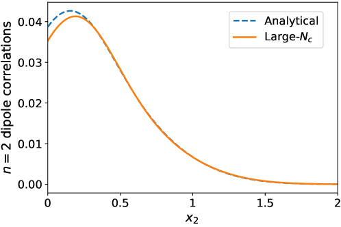
Figure 1: Validity check for the large-$N_{\mathrm{c}}$ approximation (45) as compared to the analytically exact result (31) for the $n=2$ dipole correlation with $Q_{\mathrm{s}}=5$ at ${\boldsymbol{x}_{\perp}}_{1}=(0,0)$, ${\boldsymbol{y}_{\perp}}_{1}=(0.6,0.6)$, ${\boldsymbol{x}_{\perp}}_{2}=(x_{2},0)$, ${\boldsymbol{y}_{\perp}}_{2}=(0.3,0.3)$ (in the unit of $\bar{\Lambda}$).

Figure 1 shows the validity check between Eqs. (31) and (45) for the $n=2$ dipole correlator with $N_{\mathrm{c}}=3$. The agreement generally depends on ${\boldsymbol{x}_{\perp}}_{i}$ and ${\boldsymbol{y}_{\perp}}_{i}$, but our formulae (45) work quite well for almost all ${\boldsymbol{x}_{\perp}}_{i}$ and ${\boldsymbol{y}_{\perp}}_{i}$ as long as $Q_{\mathrm{s}}$ is not too large (when $Q_{\mathrm{s}}$ is too large, the outputs are too small, and the errors become relatively larger). Here, in Fig. 1, we chose $Q_{\mathrm{s}}=5$ and ${\boldsymbol{x}_{\perp}}_{1}=(0,0)$, ${\boldsymbol{y}_{\perp}}_{1}=(0.6,0.6)$, ${\boldsymbol{x}_{\perp}}_{2}=(x_{2},0)$, ${\boldsymbol{y}_{\perp}}_{2}=(0.3,0.3)$, which is intentionally chosen to make the difference as visible as possible for the small $x_{2}$ region, and so, the overall agreement is better than shown in Fig. 1.

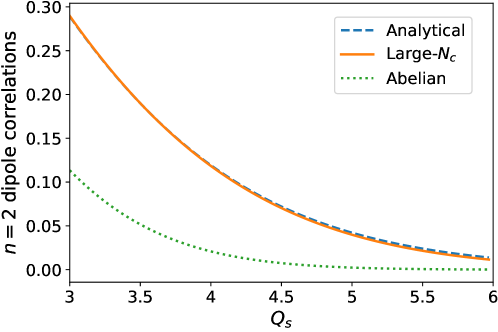
Figure 2: Validity check for the large-$N_{\mathrm{c}}$ approximation (45) and the Abelian approximation as compared to the analytically exact result (31) for the $n=2$ dipole correlation. The positions are chosen as ${\boldsymbol{x}_{\perp}}_{1}=(0,0)$, ${\boldsymbol{y}_{\perp}}_{1}=(0.6,0.6)$, ${\boldsymbol{x}_{\perp}}_{2}=(0.1,0)$, ${\boldsymbol{y}_{\perp}}_{2}=(0.3,0.3)$.

We next see the $Q_{\mathrm{s}}$ dependence of the $n=2$ dipole correlator together with the Abelian approximation, as depicted in Fig. 2. We introduce the Abelian approximation as employed in Ref. Dusling:2017dqg ; Dusling:2017aot so that the $n=1$ expectation value can reproduce the exact result. For example of the $n=2$ case, the Abelian approximation reads

$$\mathrm{e}^{-Q_{\mathrm{s}}^{2}[\Gamma(|{\boldsymbol{x}_{\perp}}_{1}-{\boldsymbol{y}_{\perp}}_{1}|)-\Gamma(|{\boldsymbol{x}_{\perp}}_{1}-{\boldsymbol{x}_{\perp}}_{2}|)+\Gamma(|{\boldsymbol{x}_{\perp}}_{1}-{\boldsymbol{y}_{\perp}}_{2}|)+\Gamma(|{\boldsymbol{x}_{\perp}}_{2}-{\boldsymbol{y}_{\perp}}_{1}|)-\Gamma(|{\boldsymbol{y}_{\perp}}_{1}-{\boldsymbol{y}_{\perp}}_{2}|)+\Gamma(|{\boldsymbol{x}_{\perp}}_{2}-{\boldsymbol{y}_{\perp}}_{2}|)]}\,,$$ (46)

which would agree with the exact answer in the limit of ${\boldsymbol{x}_{\perp}}_{1}={\boldsymbol{y}_{\perp}}_{1}$ or ${\boldsymbol{x}_{\perp}}_{2}={\boldsymbol{y}_{\perp}}_{2}$ (in which the correlator reduces to the $n=1$ one), but deviates from the exact answer for general ${\boldsymbol{x}_{\perp}}_{i}$ and ${\boldsymbol{y}_{\perp}}_{i}$. In this sense, the expression like Eq. (46) is to be regarded as an Abelianized extrapolation from the $n=1$ answer. Figure 2 clearly shows that a small disagreement magnified in Fig. 1 is actually a negligibly small difference in the whole profile over various $Q_{\mathrm{s}}$. The Abelian approximation captures a qualitative dependence with increasing $Q_{\mathrm{s}}$, while the quantitative values should be considered as only order estimates.

6 Flow harmonics and higher order contributions

We follow the calculations of the flow observables, $v_{n}\{m\}$, according to Refs. Dusling:2017dqg ; Dusling:2017aot . The flows are characteristic angular distributions defined from the $m$-particle inclusive spectra, which are in the dipole model given by

$$\begin{split}&\frac{\mathrm{d}^{m}N}{\mathrm{d}^{2}{\boldsymbol{p}_{\perp}}_{1}\cdots\mathrm{d}^{2}{\boldsymbol{p}_{\perp}}_{m}}\\ &=\frac{1}{(4\pi^{3}B)^{m}}\prod_{i=1}^{m}\int\mathrm{d}^{2}{\boldsymbol{x}_{\perp}}_{i}\,\mathrm{d}^{2}{\boldsymbol{y}_{\perp}}_{i}\,\mathrm{e}^{-\frac{{\boldsymbol{x}_{\perp}}_{i}^{2}+{\boldsymbol{y}_{\perp}}_{i}^{2}}{2B}+\mathrm{i}({\boldsymbol{x}_{\perp}}_{i}-{\boldsymbol{y}_{\perp}}_{i})\cdot{\boldsymbol{p}_{\perp}}_{i}}\biggl{\langle}\prod_{j=1}^{m}D({\boldsymbol{x}_{\perp}}_{j},{\boldsymbol{y}_{\perp}}_{j})\biggr{\rangle}\,,\end{split}$$ (47)

where $B$ is a dipole model parameter, which is typically of the order of the nucleon size $\sim 1\;\text{fm}\sim(0.2\;\text{GeV})^{-1}$, and we take $\sqrt{B}=2\;\text{GeV}^{-1}$. The general analysis for the flow properties is presented in Ref. Borghini:2001vi and the $n$-th moment of the $m$-particle correlation is introduced as

$$\kappa_{n}\{m\}:=\prod_{i=1}^{m}\int\frac{\mathrm{d}^{2}{\boldsymbol{p}_{\perp}}_{i}}{(2\pi)^{2}}\,\mathrm{e}^{\mathrm{i}n(-1)^{i+1}\phi_{i}}\,\frac{\mathrm{d}^{m}N}{\mathrm{d}^{2}{\boldsymbol{p}_{\perp}}_{1}\cdots{\boldsymbol{p}_{\perp}}_{m}}\,,$$ (48)

where $\phi_{i}$ represents the azimuthal angle, i.e. ${\boldsymbol{p}_{\perp}}_{i}=|{\boldsymbol{p}_{\perp}}_{i}|(\cos\phi_{i},\sin\phi_{i})$. Then, in the dipole model, we can perform the momentum integrations to find the following expression,

$$\begin{split}&\kappa_{n}\{m\}\\ &=\frac{1}{(4\pi^{3}B)^{m}}\prod_{i=1}^{m}\int\mathrm{d}^{2}{\boldsymbol{x}_{\perp}}_{i}\,\mathrm{d}^{2}{\boldsymbol{y}_{\perp}}_{i}\,\mathrm{e}^{-\frac{{\boldsymbol{x}_{\perp}}_{i}^{2}+{\boldsymbol{y}_{\perp}}_{i}^{2}}{2B}}K_{n}^{((-1)^{i+1})}({\boldsymbol{x}_{\perp}}_{i}-{\boldsymbol{y}_{\perp}}_{i})\biggl{\langle}\prod_{j=1}^{m}D({\boldsymbol{x}_{\perp}}_{j},{\boldsymbol{y}_{\perp}}_{j})\biggr{\rangle}\,.\end{split}$$ (49)

Here, using the regularized generalized hypergeometric function, we defined,

$$K_{n}^{(\pm)}({\boldsymbol{x}_{\perp}}) :=\int^{p_{\text{max}}}\frac{\mathrm{d}^{2}{\boldsymbol{p}_{\perp}}}{(2\pi)^{2}}\,\mathrm{e}^{\pm\mathrm{i}n\phi+\mathrm{i}{\boldsymbol{x}_{\perp}}\cdot{\boldsymbol{p}_{\perp}}}$$

$$=\frac{\mathrm{i}^{n}p_{\text{max}}^{2}\,\mathrm{e}^{\pm\mathrm{i}n\theta}}{2\pi(n+2)n!}\biggl{(}\frac{|{\boldsymbol{x}_{\perp}}|p_{\text{max}}}{2}\biggr{)}^{n}\!\!{{}_{1}F_{2}}\biggl{(}1+\frac{n}{2};\Bigl{\{}1+n,\,2+\frac{n}{2}\Bigr{\}};-\frac{1}{4}|{\boldsymbol{x}_{\perp}}|^{2}p_{\text{max}}^{2}\biggr{)}\,,$$ (50)

where $\theta$ is the azimuthal angle of ${\boldsymbol{x}_{\perp}}$. In particular, we will frequently use the $n=0$ function for the normalization, which is given by

$$K_{0}^{(\pm)}({\boldsymbol{x}_{\perp}})=\tilde{\delta}_{p_{\text{max}}}^{(2)}({\boldsymbol{x}_{\perp}}):=\frac{p_{\text{max}}}{2\pi|{\boldsymbol{x}_{\perp}}|}J_{1}(|{\boldsymbol{x}_{\perp}}|p_{\text{max}})\,.$$ (51)

It is important to notice that $\pm$ is irrelevant for $n=0$ and there is no angular dependence any more in $K_{0}^{(\pm)}({\boldsymbol{x}_{\perp}})$. Also, we must point out that $\tilde{\delta}_{p_{\text{max}}}^{(2)}({\boldsymbol{x}_{\perp}})$ should approach $\delta^{(2)}({\boldsymbol{x}_{\perp}})$ in the $p_{\text{max}}\to\infty$ limit.

Let us first consider the case with $m=2$ using our large-$N_{\mathrm{c}}$ expansion. The $N_{\mathrm{c}}^{0}$ order term in Eq. (45) does not contribute to $\kappa_{n}\{2\}$ due to the phase factor in $K_{n}^{(\pm)}({\boldsymbol{x}_{\perp}}_{i}-{\boldsymbol{y}_{\perp}}_{i})$. As a result, we can write $\kappa_{n}\{2\}$ using the $N_{\mathrm{c}}^{-2}$ order results as

$$\kappa_{n}\{2\}=D_{n}^{(+-)}\,,$$ (52)

where

$$\begin{split}D_{n}^{(+-)}&:=\frac{1}{(4\pi^{3}B)^{2}}\int\mathrm{d}^{2}{\boldsymbol{x}_{\perp}}_{1}\,\mathrm{d}^{2}{\boldsymbol{y}_{\perp}}_{1}\,\mathrm{d}^{2}{\boldsymbol{x}_{\perp}}_{2}\,\mathrm{d}^{2}{\boldsymbol{y}_{\perp}}_{2}\,\mathrm{e}^{-\frac{{\boldsymbol{x}_{\perp}}_{1}^{2}+{\boldsymbol{y}_{\perp}}_{1}^{2}+{\boldsymbol{x}_{\perp}}_{2}^{2}+{\boldsymbol{y}_{\perp}}_{2}^{2}}{2B}}\\ &\quad\times\mathrm{e}^{-Q_{\mathrm{s}}^{2}\Gamma({\boldsymbol{x}_{\perp}}_{1}-{\boldsymbol{y}_{\perp}}_{1})}K_{n}^{(+)}({\boldsymbol{x}_{\perp}}_{1}-{\boldsymbol{y}_{\perp}}_{1})\,\mathrm{e}^{-Q_{\mathrm{s}}^{2}\Gamma({\boldsymbol{x}_{\perp}}_{2}-{\boldsymbol{y}_{\perp}}_{2})}K_{n}^{(-)}({\boldsymbol{x}_{\perp}}_{2}-{\boldsymbol{y}_{\perp}}_{2})\\ &\quad\times\biggl{(}1-\frac{1-\mathrm{e}^{-\Delta E_{(21)}^{(0)}}}{\Delta E_{(21)}^{(0)}}\biggr{)}\biggl{(}\frac{V_{(21),0}^{(1)}}{N_{\mathrm{c}}}+\frac{V_{0,(21)}^{(1)}V_{(21),0}^{(1)}}{\Delta E_{(21)}^{(0)}}\biggr{)}\,.\end{split}$$ (53)

One could think of $D_{n}^{(++)}$ and $D_{n}^{(--)}$ in a similar manner but they are also vanishing because of the phase factors in $K_{n}^{(\pm)}$. The last part of the integrand is a function of modulus of various combinations of ${\boldsymbol{x}_{\perp}}_{1}$, ${\boldsymbol{x}_{\perp}}_{2}$, ${\boldsymbol{y}_{\perp}}_{1}$, ${\boldsymbol{y}_{\perp}}_{2}$. Here, it is crucially important to understand that any term in the integrand which is factorized into a function of $|{\boldsymbol{x}_{\perp}}_{i}-{\boldsymbol{y}_{\perp}}_{i}|$ alone would vanish due to the phase factors in $K_{n}^{(\pm)}({\boldsymbol{x}_{\perp}}_{i}-{\boldsymbol{y}_{\perp}}_{i})$ in the factorized integrations.

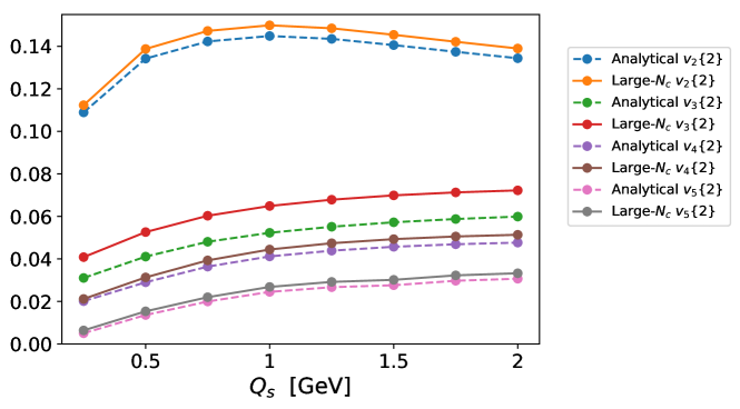
Figure 3: 2-particle flow harmonics using the analytical (unapproximated) expression (31) and our formulae (45). The saturation momentum $Q_{\mathrm{s}}$ is the one defined in Eq. (57) as in Ref. Dusling:2017aot .

Because there is no finite contribution of disconnected parts in the two particle correlation, we can immediately compute the two particle flow harmonics, $v_{n}\{2\}$, from

$$v_{n}\{2\}=\sqrt{\frac{\kappa_{n}\{2\}}{\kappa_{0}\{2\}}}\,,$$ (54)

where the denominator is obtained with Eq. (51), i.e. if we keep using the expanded expression up to the $N_{\mathrm{c}}^{-2}$ order for later convenience, we have

$$\kappa_{0}\{2\}=D_{0}^{2}+D_{0}^{(+-)}\,.$$ (55)

Here, we defined

$$D_{0}:=\frac{1}{4\pi^{3}B}\int\mathrm{d}^{2}{\boldsymbol{x}_{\perp}}\,\mathrm{d}^{2}{\boldsymbol{y}_{\perp}}\,\mathrm{e}^{-\frac{{\boldsymbol{x}_{\perp}}^{2}+{\boldsymbol{y}_{\perp}}^{2}}{2B}}\,\mathrm{e}^{-Q_{\mathrm{s}}^{2}\Gamma({\boldsymbol{x}_{\perp}}-{\boldsymbol{y}_{\perp}})}\,\tilde{\delta}_{p_{\text{max}}}^{(2)}({\boldsymbol{x}_{\perp}}-{\boldsymbol{y}_{\perp}})\,.$$ (56)

Of course, up to this order, keeping $D_{0}^{(+-)}$ in the denominator is in principle irrelevant since it gives a higher order correction which we should neglect.

We summarize our numerical results in Fig. 3. We have performed the 8 dimensional numerical integration with respect to $\{{\boldsymbol{x}_{\perp}}_{i},{\boldsymbol{y}_{\perp}}_{i}\}$ using the Monte-Carlo method by taking $10^{8}$ sampling points. To draw Fig. 3 we chose $\bar{\Lambda}=0.241\;\text{GeV}$ and $p_{\text{max}}=2\;\text{GeV}$ in accord with Ref. Dusling:2017aot . We also note that, only in this section, we change the definition of the saturation momentum from our original $Q_{\mathrm{s}}$ in Eqs. (2) and (3) to new $\bar{Q}_{\text{s}}$ defined by

$$\bar{Q}_{\text{s}}^{2}=\frac{1}{2\Gamma(|\sqrt{2}/Q_{\mathrm{s}}|)}$$ (57)

according to Refs. Dusling:2017dqg ; Dusling:2017aot . Since there is no confusion, in this section, we will omit bar and simply denote $Q_{\mathrm{s}}$ to mean $\bar{Q}_{\text{s}}$. Then, we can make a direct comparison of our outputs to Fig. 1 of Ref. Dusling:2017dqg . The dashed curved in Fig. 3 must precisely reproduce Fig. 1 of Ref. Dusling:2017dqg . At a glance of our numerical calculations we see quantitatively good agreement. The most interesting question is how useful our large-$N_{\mathrm{c}}$ formulae (45) can be for the $N_{\mathrm{c}}=3$ case. The comparison between the dashed curves (full analytical results) and the solid curves (large-$N_{\mathrm{c}}$ approximations) in Fig. 3 concludes that the errors are of only a few (at most $\sim 5$) % level except for the $n=3$ case.

Next, it is intriguing to see what happens for $m=4$. In this case, $\kappa_{n}\{4\}$ involves $K_{n}^{(+)}({\boldsymbol{x}_{\perp}}_{1}-{\boldsymbol{y}_{\perp}}_{1})$, $K_{n}^{(-)}({\boldsymbol{x}_{\perp}}_{2}-{\boldsymbol{y}_{\perp}}_{2})$, $K_{n}^{(+)}({\boldsymbol{x}_{\perp}}_{3}-{\boldsymbol{y}_{\perp}}_{3})$, and $K_{n}^{(-)}({\boldsymbol{x}_{\perp}}_{4}-{\boldsymbol{y}_{\perp}}_{4})$. It is then easy to understand that our formula of the $N_{\mathrm{c}}^{-2}$ order in Eq. (45) is insufficient to get nonvanishing contributions. Terms of the formula (45) are functions of, say, ${\boldsymbol{x}_{\perp}}_{1}$, ${\boldsymbol{x}_{\perp}}_{2}$, ${\boldsymbol{y}_{\perp}}_{1}$, ${\boldsymbol{y}_{\perp}}_{2}$ for $i=2$ and $j=1$, and then the angle integrations of ${\boldsymbol{x}_{\perp}}_{3}-{\boldsymbol{y}_{\perp}}_{3}$ and ${\boldsymbol{x}_{\perp}}_{4}-{\boldsymbol{y}_{\perp}}_{4}$ become zero. Therefore, one permutation is not enough, but two permutations are necessary to shuffle all ${\boldsymbol{x}_{\perp}}_{1}$, ${\boldsymbol{x}_{\perp}}_{2}$, ${\boldsymbol{x}_{\perp}}_{3}$, and ${\boldsymbol{x}_{\perp}}_{4}$; we must go to the next $N_{\mathrm{c}}^{-4}$ order to compute a first nonzero term in $\kappa_{n}\{4\}$.

It is a straightforward but tedious calculation to pick all the $N_{\mathrm{c}}^{-4}$ order terms up from the expansion in Eq. (42). We can slightly simplify the problem by discarding terms which do not contribute to $\kappa_{n}\{4\}$. The $N_{\mathrm{c}}^{-4}$ order terms generally contain the product of the interaction matrix elements like

$$\sim V_{0,(pq)}^{(1)}V_{(pq),(ij)(kl)}^{(1)}V_{(ij)(kl),(ij)}^{(1)}V_{(ij),0}^{(1)}\,,$$ (58)

but we already saw that, if an unexchanged pair exists, the angle integration is vanishing. For example, if the above matrix elements are $\sim V_{0,(21)}^{(1)}V_{(21),0}^{(1)}V_{0,(21)}^{(1)}V_{(21),0}^{(1)}$, which itself is nonzero, the angle integrations of ${\boldsymbol{x}_{\perp}}_{3}-{\boldsymbol{y}_{\perp}}_{3}$ and ${\boldsymbol{x}_{\perp}}_{4}-{\boldsymbol{y}_{\perp}}_{4}$ are zero. Thus, among all possible combinations of the matrix elements, there are finite contributions only from

$$\begin{split}&V_{0,(43)}^{(1)}V_{(43),(0)}^{(1)}V_{(0),(21)}^{(1)}V_{(21),0}^{(1)}\,,\qquad V_{0,(42)}^{(1)}V_{(42),(0)}^{(1)}V_{(0),(31)}^{(1)}V_{(31),0}^{(1)}\,,\\ &V_{0,(32)}^{(1)}V_{(32),(0)}^{(1)}V_{(0),(41)}^{(1)}V_{(41),0}^{(1)}\,.\end{split}$$ (59)

Here, we used relations such as $V_{(ij)(kl),(ij)}^{(1)}=V_{(kl),0}^{(1)}$, $V_{(kl),(ij)(kl)}^{(1)}=V_{0,(ij)}^{(1)}$, etc for $(ij)\neq(kl)$. After long calculations we arrive at a final form which turned out to be factorized as

$$\kappa_{n}\{4\} =\frac{1}{(4\pi^{3}B)^{4}}\prod_{i=1}^{4}\int\mathrm{d}^{2}{\boldsymbol{x}_{\perp}}_{i}\,\mathrm{d}^{2}{\boldsymbol{y}_{\perp}}_{i}\,\mathrm{e}^{-\frac{{\boldsymbol{x}_{\perp}}_{i}^{2}+{\boldsymbol{y}_{\perp}}_{i}^{2}}{2B}}\,\mathrm{e}^{-Q_{\mathrm{s}}^{2}\Gamma({\boldsymbol{x}_{\perp}}_{i}-{\boldsymbol{y}_{\perp}}_{i})}K_{n}^{((-1)^{i+1})}({\boldsymbol{x}_{\perp}}_{i}-{\boldsymbol{y}_{\perp}}_{i})$$

$$\quad\times\frac{1}{2!}\sum_{(ij)\neq(kl)}\biggl{(}1-\frac{1-\mathrm{e}^{-\Delta E_{(ij)}^{(0)}}}{\Delta E_{(ij)}^{(0)}}\biggr{)}\biggl{(}\frac{V_{(ij),0}^{(1)}}{N_{\mathrm{c}}}+\frac{V_{0,(ij)}^{(1)}V_{(ij),0}^{(1)}}{\Delta E_{(ij)}^{(0)}}\biggr{)}$$

$$\qquad\qquad\quad\;\times\biggl{(}1-\frac{1-\mathrm{e}^{-\Delta E_{(kl)}^{(0)}}}{\Delta E_{(kl)}^{(0)}}\biggr{)}\biggl{(}\frac{V_{(kl),0}^{(1)}}{N_{\mathrm{c}}}+\frac{V_{0,(kl)}^{(1)}V_{(kl),0}^{(1)}}{\Delta E_{(kl)}^{(0)}}\biggr{)}\,,$$ (60)

which is the full expression of the $N_{\mathrm{c}}^{-4}$ order without any truncation like the glasma graph approximation. This result looks quite reasonable, but we emphasize that the complete cancellation of $(ij)(kl)$ intermediate states with an energy denominator, $E_{(ij)}+E_{(kl)}$, is far from trivial. The sum with respect to $(ij)$ and $(kl)$ should run over all the permutations of the combinations as listed in Eq. (59). Among all the combinations of indices, $[(ij)=(31),(kl)=(42)]$ and $[(ij)=(42),(kl)=(31)]$ are irrelevant because $D_{n}^{(++)}=D_{n}^{(--)}=0$ (for $n>0$) as we already pointed out. Therefore, the remaining four combinations of $[(ij)=(21),(kl)=(43)]$, $[(ij)=(43),(kl)=(21)]$, $[(ij)=(41),(kl)=(32)]$, and $[(ij)=(32),(kl)=(41)]$ lead to

$$\kappa_{n}\{4\}=2\bigl{[}D_{n}^{(+-)}\bigr{]}^{2}\,.$$ (61)

Then, with extra terms corresponding to $D_{0}^{(++)}$ and $D_{0}^{(--)}$ which are nonzero, the normalization is written as

$$\kappa_{0}\{4\}=D_{0}^{4}+6D_{0}^{2}D_{0}^{(+-)}\,,$$ (62)

up to the $N_{\mathrm{c}}^{-2}$ order in the same way as in Eq. (55). Now, the cumulant is then given by

$$c_{n}\{4\}=\frac{\kappa_{n}\{4\}}{\kappa_{0}\{4\}}-2\biggl{(}\frac{\kappa_{n}\{2\}}{\kappa_{0}\{2\}}\biggr{)}^{2}\,.$$ (63)

The above quantity itself is zero in the strict order counting for $c_{n}\{4\}$ up to $N_{\mathrm{c}}^{-4}$. Thus, our conclusion is, even in the full MV model beyond the glasma graph approximation, no connected cumulant remains for $c_{n}\{4\}$ at the $N_{\mathrm{c}}^{-4}$ order.

In this way we can understand that the first connected contribution to cumulants appears from the $N_{\mathrm{c}}^{-2m+2}$ order; for $m=4$, thus, we need to go to the $N_{\mathrm{c}}^{-6}$ order and then a completely nested combination of four indices like $(43),(32),(21)$ is possible. Therefore, the flow harmonics from the fully nested permutations must scale as

$$v_{n}\{m\}\sim N_{\mathrm{c}}^{-2+2/m}\,.$$ (64)

This is our conclusion on the $N_{\mathrm{c}}$ scaling in the full MV model.

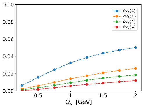
Figure 4: $\delta v_{n}\{4\}$ estimated from Eq. (66) using $v_{n}\{2\}$ obtained in the large-$N_{\mathrm{c}}$ limit. Our choice of the parameter is $p_{\text{max}}=2\;\text{GeV}$.

Although our conclusion of $c_{n}\{4\}=0$ at the $N_{\mathrm{c}}^{-4}$ order is solid, there may be a subtle point in the large-$N_{\mathrm{c}}$ scaling due to finiteness of $p_{\text{max}}$. If one just uses our formulae up to the $N_{\mathrm{c}}^{-4}$ order to estimate $\kappa_{n}\{2\}$, $\kappa_{0}\{2\}$, $\kappa_{n}\{4\}$, and $\kappa_{0}\{4\}$, one would naïvely find that the cancellation is incomplete at the $N_{\mathrm{c}}^{-6}$ order and a finite remainder is given by

$$\delta c_{n}\{4\}=\frac{2[D_{n}^{(+-)}]^{2}}{D_{0}^{4}+6D_{0}^{2}D_{0}^{(+-)}}-2\biggl{(}\frac{D_{n}^{(+-)}}{D_{0}^{2}+D_{0}^{(+-)}}\biggr{)}^{2}\simeq-\frac{8[D_{n}^{(+-)}]^{2}D_{0}^{(+-)}}{D_{0}^{6}}\simeq-\frac{8D_{0}^{(+-)}}{D_{0}^{2}}(v_{n}\{2\})^{4}\,.$$ (65)

This correction is beyond the $N_{\mathrm{c}}^{-4}$ order and should be identified as a part of the $N_{\mathrm{c}}^{-6}$ terms. One can easily check that this $N_{\mathrm{c}}^{-6}$ order correction is vanishing for $p_{\text{max}}\to\infty$, in which $D_{0}^{(+-)}\to 0$. However, for a finite $p_{\text{max}}$ especially comparable to $Q_{\mathrm{s}}$, the correction could be sizable and the flow harmonics is modified even from the disconnected piece. To see this effect quantitatively, let us compute the flow harmonics corresponding to $\delta c\{4\}$, which leads to

$$\delta v_{n}\{4\}=(-\delta c_{n}\{4\})^{1/4}=2^{3/4}\biggl{(}\frac{D_{0}^{(+-)}}{D_{0}^{2}}\biggr{)}^{1/4}v_{n}\{2\}\,.$$ (66)

We make a plot of $\delta v_{n}\{4\}$ as a function of $Q_{\mathrm{s}}$ in Fig. 4. One must be very careful of the physical interpretation of this correction by $\delta v_{n}\{4\}$. Even though this is non-negligible as seen in Fig. 4, the physical origin lies in not the connected correlator but in the normalization. Moreover, this normalization effect makes the $N_{\mathrm{c}}$ counting skewed to become

$$\delta v_{n}\{m\}\sim N_{\mathrm{c}}^{-1-2/m}\qquad(m\geq 4)\,,$$ (67)

which starts differing from anticipated Eq. (64) for $m>4$. Thus, to distinguish the connected contribution from the normalization effect, one can test the $N_{\mathrm{c}}$ scaling properties as in Eqs. (64) and (67) and also check the $p_{\text{max}}$ dependence since $\delta v_{n}\{m\}$ from the normalization effect is very sensitive to $p_{\text{max}}/Q_{\mathrm{s}}$ as perceived from Fig. 4.

7 Conclusions

We have established general formulae and machineries to compute $2n$-point Wilson line (or $n$ dipole) correlators with the color group representation $(N_{\mathrm{c}}\otimes\bar{N_{\mathrm{c}}})^{n}$ in the McLerran-Venugopalan model. The color structure accommodates a huge representation but the nonzero contribution to the Wilson line correlators reduces to the $n!\times n!$ matrix, whose bases correspond to the color singlets. In particular, we have derived the explicit expression of the matrix elements [see Eqs. (26) and (27)] in the color singlet bases constructed by permutations. The formulae are quite powerful not only for the direct numerical evaluation of the matrix but also for the analytical large-$N_{\mathrm{c}}$ expansion. We have developed the systematic large-$N_{\mathrm{c}}$ expansion in a way analogous to time-dependent perturbation theory in quantum mechanics. We have then shown the explicit expression up to $N_{\mathrm{c}}^{-2}$ order for the dipole correlators as given in Eq. (45). As a check of the validity, we have compared results from the exact answers and those in the large-$N_{\mathrm{c}}$ expansion for the two-particle flow harmonics, $v_{n}\{2\}$ $(n=2,3,4,5)$, which shows quantitatively good agreement. We have continued our large-$N_{\mathrm{c}}$ expansion to higher orders to discuss the flow harmonics with more particles. Then, we have discovered the $N_{\mathrm{c}}$ scaling as $v_{n}\{m\}\sim N_{\mathrm{c}}^{-2+2/m}$ even beyond the glasma graph approximation but in the full MV model. We have also pointed out that a slightly different $N_{\mathrm{c}}$ scaling could emerge from the normalization effect at finite cutoff of the transverse momenta of integrated particles.

Although we focused on only the dipole correlators in the present paper, our general formulae also provide us with useful approaches to evaluate Wilson line correlators in channels relevant for the particle production rate in the $p$-$A$ collision generally. In fact, not only fundamental but also adjoint Wilson line correlators appearing in the multi-gluon production can be derived from our results in Eq. (1) through the relation $[U_{\text{adj}}]_{ba}({\boldsymbol{x}_{\perp}})=2\mathrm{tr}[U({\boldsymbol{x}_{\perp}}){T_{\mathrm{F}}}^{a}U^{{\dagger}}({\boldsymbol{x}_{\perp}}){T_{\mathrm{F}}}^{b}]={T_{\mathrm{F}}}_{\alpha\bar{\alpha}}^{a}{T_{\mathrm{F}}}_{\bar{\beta}\beta}^{b}U_{\beta\alpha}({\boldsymbol{x}_{\perp}})U_{\bar{\beta}\bar{\alpha}}^{*}({\boldsymbol{x}_{\perp}})$.

As we emphasized, our scheme of the large-$N_{\mathrm{c}}$ expansion takes a nice form which is easily implemented in numerical algorithms to go to arbitrarily higher orders. Such higher order numerical evaluations are left as an intriguing future problem. It would be also an important question to think about generalizations beyond the MV model. Further systematic considerations on the Wilson line correlators should deserve more investigations in the future.

References

(1)
A. H. Mueller, Soft gluons in the infinite momentum wave function and
the BFKL pomeron,
Nucl. Phys.B415 (1994) 373–385.
(13)
J. Jalilian-Marian, A. Kovner, A. Leonidov and H. Weigert, The Wilson
renormalization group for low x physics: Towards the high density regime,
Phys. Rev.D59 (1998) 014014,
[hep-ph/9706377].
(14)
J. Jalilian-Marian, A. Kovner and H. Weigert, The Wilson renormalization
group for low x physics: Gluon evolution at finite parton density,
Phys. Rev.D59 (1998) 014015,
[hep-ph/9709432].
(15)
Y. V. Kovchegov, NonAbelian Weizsacker-Williams field and a
two-dimensional effective color charge density for a very large nucleus,
Phys. Rev.D54 (1996) 5463–5469,
[hep-ph/9605446].
(20)
T. Lappi and H. Mantysaari, Direct numerical solution of the coordinate
space Balitsky-Kovchegov equation at next to leading order,
Phys. Rev.D91 (2015) 074016,
[1502.02400].
(22)
T. Lappi and H. Mantysaari, Forward dihadron correlations in
deuteron-gold collisions with the Gaussian approximation of JIMWLK,
Nucl. Phys.A908 (2013) 51–72,
[1209.2853].
(25)
J. P. Blaizot, F. Gelis and R. Venugopalan, High-energy pA collisions in
the color glass condensate approach. 1. Gluon production and the Cronin
effect,
Nucl. Phys.A743 (2004) 13–56,
[hep-ph/0402256].
(26)
J. P. Blaizot, F. Gelis and R. Venugopalan, High-energy pA collisions in
the color glass condensate approach. 2. Quark production,
Nucl. Phys.A743 (2004) 57–91,
[hep-ph/0402257].
(29)
K. Fukushima and Y. Hidaka, Two Gluon Production and Longitudinal
Correlations in the Color Glass Condensate,
Nucl. Phys.A813 (2008) 171–197,
[0806.2143].
(30)
J. L. Albacete and C. Marquet, Azimuthal correlations of forward
di-hadrons in d+Au collisions at RHIC in the Color Glass Condensate,
Phys. Rev.
Lett.105 (2010) 162301,
[1005.4065].
(31)
A. Kovner, M. Lublinsky and V. Skokov, Exploring correlations in the CGC
wave function: odd azimuthal anisotropy,
1612.07790.
(36)
S. Benic, K. Fukushima, O. Garcia-Montero and R. Venugopalan, Probing
gluon saturation with next-to-leading order photon production at central
rapidities in proton-nucleus collisions,
JHEP01
(2017) 115, [1609.09424].
(37)
A. Dumitru, F. Gelis, L. McLerran and R. Venugopalan, Glasma flux tubes
and the near side ridge phenomenon at RHIC,
Nucl. Phys.A810 (2008) 91–108,
[0804.3858].
(38)
A. Dumitru, K. Dusling, F. Gelis, J. Jalilian-Marian, T. Lappi and
R. Venugopalan, The Ridge in proton-proton collisions at the LHC,
Phys. Lett.B697 (2011) 21–25,
[1009.5295].
(40)
V. Skokov, High order cumulants of the azimuthal anisotropy in the
dilute-dense limit: Connected graphs,
Phys. Rev.D91 (2015) 054014,
[1412.5191].
(41)
T. Lappi, B. Schenke, S. Schlichting and R. Venugopalan, Tracing the
origin of azimuthal gluon correlations in the color glass condensate,
JHEP01
(2016) 061, [1509.03499].
(42)
K. Dusling, M. Mace and R. Venugopalan, Multiparticle collectivity from
initial state correlations in high energy proton-nucleus collisions,
1705.00745.
(43)
K. Dusling, M. Mace and R. Venugopalan, Parton model description of
multiparticle azimuthal correlations in collisions,
1706.06260.
(44)
Y. Shi, C. Zhang and E. Wang, Multipole scattering amplitudes in the
Color Glass Condensate formalism,
Phys. Rev.D95 (2017) 116014,
[1704.00266].
(45)
K. Fukushima and Y. Hidaka, Light projectile scattering off the color
glass condensate,
JHEP06 (2007) 040, [0704.2806].
(46)
A. Dumitru and V. Skokov, Fluctuations of the gluon distribution from
the small-x effective action,
1704.05917.