A Unified Model for Near and Remote Sensing

Abstract

We propose a novel convolutional neural network architecture for estimating geospatial functions such as population density, land cover, or land use. In our approach, we combine overhead and ground-level images in an end-to-end trainable neural network, which uses kernel regression and density estimation to convert features extracted from the ground-level images into a dense feature map. The output of this network is a dense estimate of the geospatial function in the form of a pixel-level labeling of the overhead image. To evaluate our approach, we created a large dataset of overhead and ground-level images from a major urban area with three sets of labels: land use, building function, and building age. We find that our approach is more accurate for all tasks, in some cases dramatically so.

1 Introduction

From predicting the weather to planning the future of our cities to recovering from natural disasters, accurately monitoring widespread areas of the Earth’s surface is essential to many scientific fields and to society in general. These observations have traditionally been collected through remote sensing from satellites, aerial imaging, and distributed observing stations and sensors. These approaches can observe certain properties like land cover and land use accurately and at a high resolution, but unfortunately, not everything can be seen from overhead imagery. For example, Wang et al. [28] evaluate approaches for urban zoning and building height estimation from overhead imagery, and conclude that urban zoning segmentation “is an extremely hard task from aerial views,” that building height estimation is “either too hard, or more sophisticated methods are needed,” and that “utilizing ground imagery seems a logical first step.”

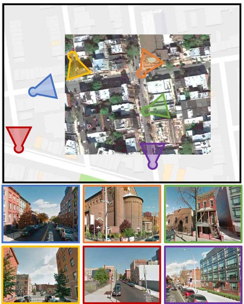
Figure 1: We use overhead imagery and geotagged ground-level imagery as input to an end-to-end deep network that estimates the values of a geospatial function by performing fine-grained pixel-level labeling on the overhead image.

More recently, the explosive popularity of geotagged social media has raised the possibility of using online user-generated content as a source of geospatial information, sometimes called image-driven mapping or proximate sensing. For example, online images from social network and photo sharing websites have been used to estimate land cover for large geographic regions [15, 38], to observe the state of the natural world by recreating maps of snowfall [27], and to quantify perception of urban environments [4]. Despite differing applications, these papers all wish to estimate some unobservable geospatial function, and view each social media artifact (e.g., geotagged ground-level image) as an observation of this function at a particular geographic location.

The typical approach [2, 33] is to (1) collect a large number of samples, (2) use an automated approach to estimate the value of the geospatial function for each sample, and (3) use some form of locally weighted averaging to interpolate the sparse samples into a dense, coherent estimate of the underlying geospatial function. This estimation is complicated by the fact that observations are noisy; state-of-the-art recognition algorithms are imperfect, some images are inherently confusing or ambiguous, and the observations are distributed sparsely and non-uniformly. This means that in order to estimate geospatial functions with reasonable accuracy, most techniques use a kernel with a large bandwidth to smooth out the noise, which yields coarse, low-resolution outputs. Despite this limitation, the proximate sensing approach can work well if ground-level imagery is plentiful, the property is easily estimated from the imagery, and the geospatial function is smoothly varying.

We propose a novel neural network architecture that combines the strengths of these two approaches (Figure 1). Our approach uses deep convolutional neural networks (CNNs) to extract features from both overhead and ground-level imagery. For the ground-level images, we use kernel regression and density estimation to convert the sparsely distributed feature samples into a dense feature map spatially consistent with the overhead image. This differs from the proximate sensing approach, which uses kernel regression to directly estimate the geospatial function. Then, we fuse the ground-level feature map with a hidden layer of the overhead image CNN. To extend our methods to pixel-level labeling, we extract multiscale features in the form of a hypercolumn and use a small neural network to estimate the geospatial function of interest. A novel element of our approach is the use of a spatially varying kernel that depends on features extracted from the overhead imagery.

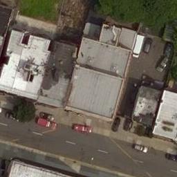
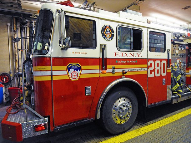
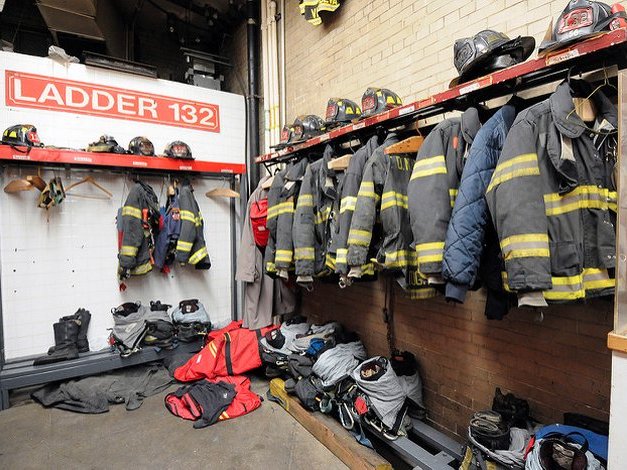
Figure 2: What type of building is shown in the overhead view (left)? Identifying and mapping building function is a challenging task that becomes considerably easier when taking into context nearby ground-level imagery (right).

Our network is trained end-to-end, so that all free parameters, including kernel bandwidths and low-level image features, are automatically tuned to minimize our loss function. In addition, our architecture is very general because it could be used with most state-of-the-art CNNs, and could be easily adapted to use any sparsely distributed media, including geotagged audio, video, and text (e.g., tweets). We evaluate our approach with a large real-world dataset, consisting of most of two major boroughs of New York City (Brooklyn and Queens), on estimating three challenging labels (building age, building function, and land use), all of which are notoriously challenging tasks in remote sensing (Figure 2). The results show that our technique for fusing overhead and ground-level imagery is more accurate than either the remote or proximate sensing approach alone, and that our automatically-estimated spatially-varying kernel improves accuracy compared to one that is uniform. The dataset and our implementation will be made available at our project website.

2 Related Work

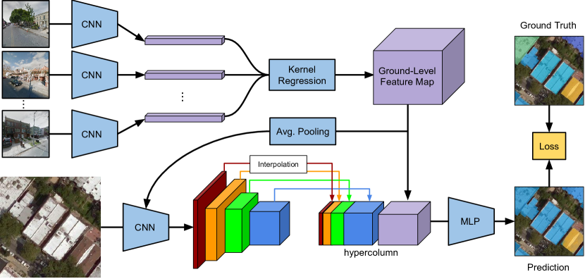
Figure 3: An overview of our network architecture.

Many recent studies have explored analyzing large-scale image collections as a means of characterizing properties of the physical world. A number of papers have tried to estimate properties of weather from geotagged and time-stamped ground-level imagery. For example, Murdock et al. [22, 21] and Jacobs et al. [11] use webcams to infer cloud cover maps, Li et al. [16] use ground-level photos to estimate smog conditions, Glasner et al. [8] estimate temperature, Zhou et al. [37] and Lee et al. [14] estimate demographic properties, Fedorov et al. [5, 6] and Wang et al. [27] infer snow cover, Khosla et al. [12] and Porzi et al. [23] measure perceived crime levels, Leung and Newsam [15] estimate land use, and so on.

Many of these papers’ contribution is exploring a novel application, as opposed to proposing novel techniques. They mostly follow a very similar recipe in which standard recognition techniques are applied to individual images, and then spatial smoothing and other noise reduction techniques are used to create an estimate of the geospatial function across the world. Meanwhile, remote sensing has long used computer vision to estimate properties of the Earth from satellite images. Of course, overhead imaging is quite different from ground-level imaging, and so remote sensing techniques have largely been developed independently and in task-specific ways [24].

We know of relatively little work that has proposed general frameworks for estimating geospatial functions from imagery, or in integrating visual evidence from both ground-level and overhead image viewpoints. Tang et al. [26] show how location context can improve image classification, but they do not use overhead imagery and their goal is not to estimate geospatial functions. Luo et al. [19] use overhead imagery to give context for event recognition in ground-level photos by combining hand-crafted features for each modality. Xie et al. [34] use transfer learning to extract socioeconomic indicators from overhead imagery. Most similar is our work on mapping the subjective attribute of natural beauty [32] where we propose to use a multilayer perceptron to combine high-level semantic features. Recent work in image geolocalization has matched ground-level photos taken at unknown locations to georegistered overhead views [17, 18, 30, 31], but this goal is significantly different from inferring geospatial functions of the world.

Several recent papers jointly reason about co-located ground-level and overhead image pairs. Máttyus et al. [20] perform joint inference over both monocular aerial and ground-level images from a stereo camera for fine-grained road segmentation, while Wegner et al. [29] detect and classify trees using features extracted from overhead and ground-level images. Ghouaiel and Lefèvre [7] transform ground-level panoramas to an overhead perspective for change detection. Zhai et al. [35] propose a transformation to extract meaningful features from overhead imagery.

In contrast with the above work, our goal is to produce a general framework for learning that can estimate any given geospatial function of the world. We integrate data from both ground-level imagery, which often contains visual evidence that is not visible from the air, and overhead imagery, which is typically much denser. We demonstrate how our models learn in an end-to-end way, avoiding the need for task-specific or hand-engineered features.

3 Problem Statement

We address the problem of estimating a spatially varying property of the physical world, which we model as an unobservable mathematical function that maps latitude-longitude coordinates to possible values of the property, $F:\mathbb{R}^{2}\rightarrow{\cal Y}$. The range ${\cal Y}$ of this function depends on the attribute to be estimated, and might be categorical (e.g., a discrete set of elements for land use classification — golf course, residential, agricultural, etc.) or continuous (e.g., population density). We wish to estimate this function based on the available observable evidence, including data sampled both densely (such as overhead imagery) and sparsely (such as geotagged ground-level images). From a probabilistic perspective, we can think of our task as learning a conditional probability distribution $P(F(l)=y|S_{l},\mathbf{G}(l))$, where $l$ is a latitude-longitude coordinate, $S_{l}$ is an overhead image centered at that location, and $\mathbf{G}(l)$ is a set of nearby ground-level images.

4 Network Architecture

We propose a novel convolutional neural network (CNN) that fuses high-resolution overhead imagery and nearby ground-level imagery to estimate the value of a geospatial function at a target location. While we focus on images, our overall architecture could be used with many sources of dense and sparse data. Our network can be trained in an end-to-end manner, which enables it to learn to optimally extract features from both the dense and sparse data sources.

4.1 Architecture Overview

The overall architecture of our network (Figure 3) consists of three main components, the details of which we describe in the next several sections: (1) constructing a spatially dense feature map using features extracted from the ground-level images (Section 4.2), (2) extracting features from the overhead image, incorporating the ground-level image feature map (Section 4.3), and (3) predicting the geospatial function value based on a hypercolumn of features (Section 4.4). A novel element of our proposed approach is the use of an adaptive, spatially varying interpolation method for constructing the ground-level image feature map based on features extracted from the overhead image (Section 4.5).

4.2 Ground-Level Feature Map Construction

The goal of this component is to convert a sparsely sampled set of ground-level images into a dense feature map. For a given geographic location $l$, let $\mathbf{G}(l)=\{(G_{i},{l_{i}})\}$ be a set of $N$ elements corresponding to the closest ground-level images, where each $(G_{i},l_{i})$ is an image and its respective geographic location. We use a CNN to extract features, $f_{g}(G_{i})$, from each image and interpolate using Nadaraya–Watson kernel regression,

$$f_{G}(l)=\frac{\sum w_{i}f_{g}(G_{i})}{\sum w_{i}},$$ (1)

where $w_{i}=exp(-d(l,l_{i};\Sigma)^{2})$ is a Gaussian kernel function where a diagonal covariance matrix $\Sigma$ controls the kernel bandwidth and $d(l,l_{i};\Sigma)$ is the Mahalanobis distance from $l$ to $l_{i}$. We perform this interpolation for every pixel location in the overhead image. The result is a feature map of size $H\times W\times m$, where $H$ and $W$ are the height and width of the overhead image in pixels, and $m$ is the output dimensionality of our ground-level image CNN.

The diagonal elements of the covariance matrix are represented by a pair of trainable weights, which pass through a softplus function (i.e. $f(x)=ln(1+e^{x})$) to ensure they are positive. Here, the value of $\Sigma$ does not depend on geographic location, a strategy we call uniform. In Section 4.5, we propose an approach in which $\Sigma$ is spatially varying.

In our experiments, the ground-level images, $\mathbf{G}(l)$, are actually geo-oriented street-level panoramas. To form a feature representation for each panorama, $G_{i}$, we first extract perspective images in the cardinal directions, resulting in four ground-level images per location. We replicate the ground-level image CNN, $f_{g}(G_{i})$, four times, feed each image through separately, and concatenate the individual outputs. We then add a final $1\times 1$ convolution to reduce the feature dimensionality. For our experiments, we use the VGG-16 architecture [25], initialized with weights for Place categorization [36] ($m=205$, layer name ‘fc8’). The result is an 820 dimensional feature vector for each location, which is further reduced to 50 dimensions.

It is possible that the nearest ground-level image may be far away, which could lead to later processing stages incorrectly interpreting the feature map. To overcome this, we concatenate a kernel density estimate, using the kernel defined in equation (1), of the ground-level image locations to the ground-level image feature map. The result is an $H\times W\times 51$ feature map that captures appearance and distributional information of the ground-level images.

     

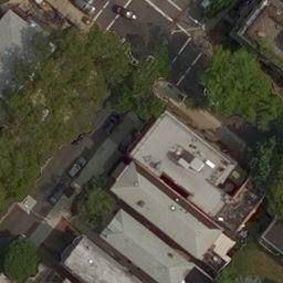
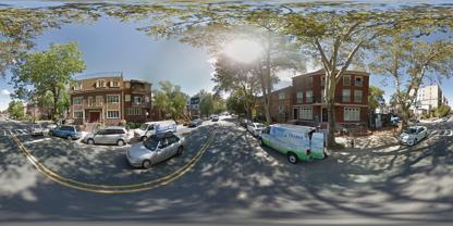
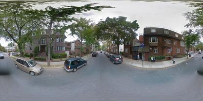
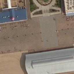
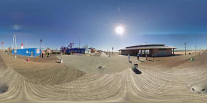
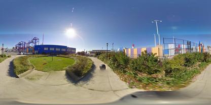
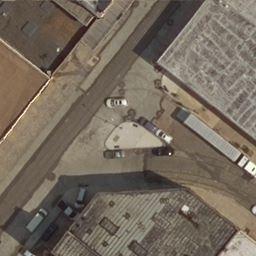
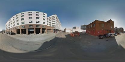
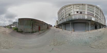
Figure 4: Sample overhead imagery and nearby street-level panoramas included in the Brooklyn and Queens dataset.

4.3 Overhead Feature Map Construction

This section describes the CNN we use to extract features from the overhead image and how we integrate the ground-level feature map. The CNN is based on the VGG-16 architecture [25], which has 13 convolutional layers, each using $3\times 3$ convolutions, and three fully connected layers. We only use the convolutional layers, typically referred to as conv-$\{1_{1-2},2_{1-2},3_{1-3},4_{1-3},5_{1-3}\}$. In addition, we reduce the dimensionality of the feature maps that are output by each layer. These layers have output dimensionality of $\{32,64,128,256,512\}$ channels, respectively. Each intermediate layer uses a leaky ReLU activation function ($\alpha=0.2$).

To fuse the ground-level feature map with the overhead imagery, we apply average pooling with a kernel size of $6\times 6$ and a stride of 2. Given an input overhead image with $H=W=256$, this reduces the ground-level feature map to $32\times 32\times 51$. We then concatenate it, in the channels dimension, with the overhead image feature map at the seventh convolutional layer, $3_{3}$. The input to convolutional layer $4_{1}$ is then $32\times 32\times 179$. We experimented with including the ground-level feature map earlier and later in the network and found this to be a good tradeoff between computational cost and expressiveness.

4.4 Geospatial Function Prediction

Given an overhead image, $S_{l}$, we use the ground-level and overhead feature maps defined above as input to the final component of our system to estimate the value of the geospatial function, $F(l(p))\in{1\ldots K}$, where $l(p)$ is the location of a pixel $p$. This pixel might be the center of the image for the image classification setting or any arbitrary pixel in the pixel-level labeling setting. To accomplish this we adapt ideas from the PixelNet architecture [3], due to its strong performance and ability to train using sparse inputs. However, our approach for incorporating sparsely distributed inputs could be adapted to other semantic labeling architectures.

We first resize each feature map to be $H\times W$ using bilinear interpolation. We then extract a hypercolumn [9] consisting of a set of features centered around $p$, $h_{p}(S)=[c_{1}(S,p),c_{2}(S,p),\ldots,...c_{M}(S,p)]$, where $c_{i}$ is the feature map of the $i$-th layer. For this work, we extract hypercolumn features from conv-$\{1_{2},2_{2},3_{3},4_{3},5_{3}\}$ and the ground-level feature map. The resulting hypercolumn feature has length 1,043. Note that resizing all intermediate feature maps to be the size of the image is quite memory intensive. Following Bansal et al. [3], we subsample pixels during training to increase the number (and therefore diversity) of images per mini-batch. At testing time, we can either compute the hypercolumn for all pixels to create a dense semantic labeling or a subset to label particular locations.

This hypercolumn feature is then passed to a small multilayer perceptron (MLP) that provides the estimate of the geospatial function. The MLP has three layers of size 512, 512, and $K$ (the task dependent number of outputs). Each intermediate layer uses a leaky ReLU activation function.

4.5 Adaptive Kernel Bandwidth Estimation

In addition to the uniform kernel described above for forming the ground-level image feature map (Section 4.2), we propose an adaptive strategy that predicts the optimal kernel bandwidth parameters for each location in the feature map. We estimate these bandwidth parameters using a CNN applied to the overhead image. This network shares the first three groups of convolutional layers, conv-$\{1_{1},\ldots,3_{3}\}$, with the overhead image CNN defined in Section 4.3. The output of these convolutions is passed to a sequence of three convolutional transpose layers, each with filter size $3\times 3$ and a stride of 2. These layers have output dimensionality of 32, 16, and 2, respectively. The final layer has an output size of $H\times W\times 2$, which represents the diagonal entries of the kernel bandwidth matrix, $\Sigma$, for each pixel location. Similar to the uniform approach, we apply a softplus activation on the output (initialized with a small constant bias) to ensure positive kernel bandwidth. When using the adaptive strategy, these bandwidth parameters are used to construct the ground-level feature map ($H\times W\times 51$).

5 Experiments

We evaluated the performance of our approach on a challenging real-world dataset, which includes overhead imagery, ground-level imagery, and several fine-grained pixel-level labels. We proposed two variants of our approach: unified (uniform), which uses a single kernel bandwidth for the entire region, and unified (adaptive), which uses a location-dependent kernel that is conditioned on the overhead image.

5.1 Baseline Methods

In order to evaluate the proposed macro-architecture, we use several baseline methods that share many low-level components with our proposed methods.

• random represents random sampling from the prior distribution of the training dataset.

• remote represents the traditional remote sensing approach, in which only overhead imagery is used. We use the unified (uniform) architecture, but do not incorporate the ground-level feature map in the overhead image CNN or the hypercolumn.

• proximate represents the proximate sensing approach in which only ground-level imagery is used. We start from the unified (uniform) architecture but only include the ground-level image feature map (minus the kernel density estimate) in the hypercolumn.

• grid is similar to the proximate method. Starting from unified (uniform), we omit all layers from the overhead image CNN prior to concatenating in the ground-level feature map from the hypercolumn. The motivation for this method is that the additional convolutional layers are able to capture spatial patterns which the final MLP cannot, because it operates on individual hypercolumns.

5.2 Implementation Details

All methods were implemented using Google’s TensorFlow framework [1] and optimized using ADAM [13] with default training parameters, except for an initial learning rate of $10^{-3}$ (decreasing by $0.5$ every 7,500 mini-batches) and weight decay of $5\times 10^{-4}$. During training, we randomly sampled 2,000 pixels per image per mini-batch. The ground-level CNNs have shared weights. All other network weights were randomly initialized and allowed to vary freely. We applied batch normalization [10] (decay $=0.99$) in all convolutional and fully connected layers (except for output layers). For our experiments, we minimize a cross entropy loss function and consider the nearest 20 street-level panoramas. Each network was trained for 25 epochs with a batch size of 32 on an NVIDIA Tesla P100.

5.3 Brooklyn and Queens Dataset

We introduce a new dataset containing ground-level and overhead images from Brooklyn and Queens, two boroughs of New York City (Figure 4). It consists of non-overlapping overhead images downloaded from Bing Maps (zoom level 19, approximately $30cm$ per pixel) and street-level panoramas from Google Street View. From Brooklyn, we collected imagery for the entirety of King’s County. This resulted in 73,921 overhead images and 139,327 panoramas. A significant number (30,316) of the overhead images are over water; we discard these and only consider those which contain buildings. We hold out 4,361 overhead images for testing. For Queens, we selected a held out region solely for evaluation and used the same process to collect imagery. This resulted in a dataset with 10,044 overhead images and 38,603 panoramas.

Using data made publicly available by NYC Open Data, we constructed a per-pixel labeling of each overhead image for the following set of labels.

Building Function.

We used 206 building classes, as outlined by the New York City Department of City Planning (NYCDCP) in the Primary Land Use Tax Lot Output (PLUTO) dataset, to categorize each building in a given overhead image. PLUTO contains detailed geographic data at the tax lot level (property boundary) for every piece of land in New York City. Example labels include: Multi-Story Department Stores, Funeral Home, and Church. To this set we add two classes, background (non-building, such as roads and water) and unknown, as there are several thousand unlabeled tax lots. To form our final labeling, we intersected the tax lot data with building footprints obtained from the NYC Planimetric Database. For reference, there are approximately 331,000 buildings in Brooklyn.

Land Use.

From PLUTO, we generated a per-pixel label image with each contained tax lot labeled according to its primary land use category. The land use categories were specified by the New York City Department of City Planning. In total, there are 11 land use categories. Example land use categories include: One and Two Family Buildings, Commercial and Office Buildings, and Open Space and Outdoor Recreation. Similar to building function, we add two classes, background (e.g., roads) and unknown.

Building Age.

Again using PLUTO in conjunction with the NYC Planimetric Database, we generated a per-pixel label image with each building labeled according to the year that construction of the building was completed. Brooklyn and Queens have a lengthy history, with the oldest building on record dating to the mid-1600s. We quantize time by decades, with a bin for all buildings constructed before 1900. This resulted in 13 bins, to which we added a bin for background (non-building), as well as unknown for a small number of buildings without a documented construction year.

5.4 Semantic Segmentation

We report results using pixel accuracy and region intersection over union averaged over classes (mIOU), two standard metrics for the semantic segmentation task. In both cases, higher is better. When computing these metrics, we ignore any ground-truth pixel labeled as unknown. In addition, for the tasks of building function and age estimation, we ignore background pixels.

ground truth
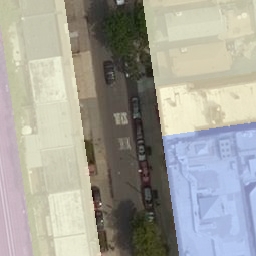
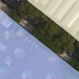
proximate
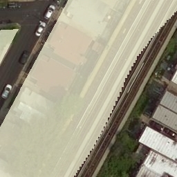
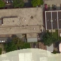
remote
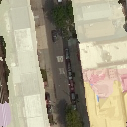
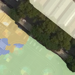
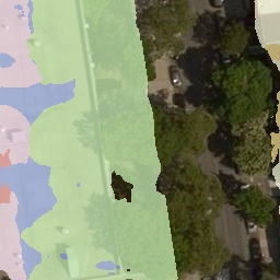
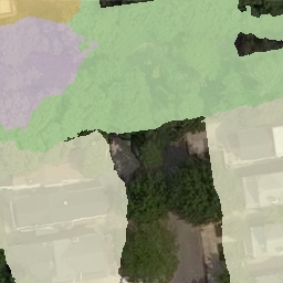
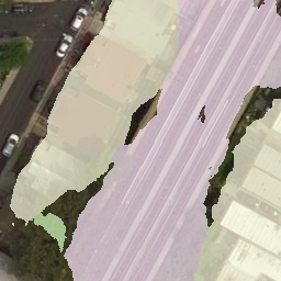
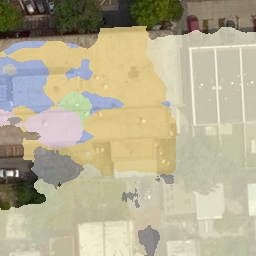
unified (adaptive)

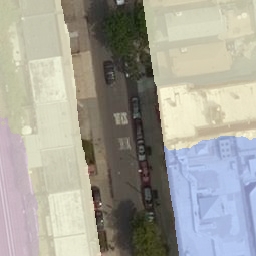
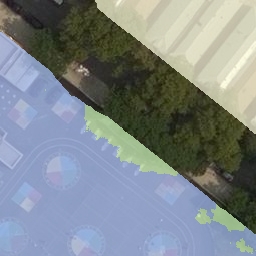
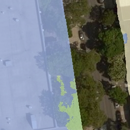
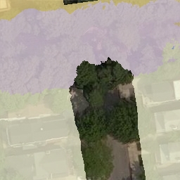
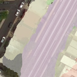
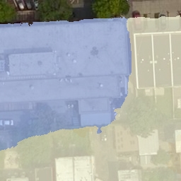
Figure 5: Sample results for classifying land use: (top–bottom) ground truth, proximate, remote, and unified (adaptive).

Table 1: Brooklyn evaluation results (top-1 accuracy).

	Age	Function	Land Use
random	6.82%	0.49%	8.55%
proximate	35.90%	27.14%	44.66%
grid	38.68%	33.84%	71.64%
remote	37.18%	34.64%	69.63%
unified (uniform)	44.08%	43.88%	76.14%
unified (adaptive)	43.85%	44.88%	77.40%

Table 2: Brooklyn evaluation results (mIOU).

	Age	Function	Land Use
random	2.76%	0.11%	3.21%
proximate	11.77%	5.46%	18.04%
grid	16.98%	9.37%	37.76%
remote	15.11%	4.67%	31.70%
unified (uniform)	20.88%	13.66%	43.53%
unified (adaptive)	23.13%	14.59%	45.54%

Table 3: Queens evaluation results (top-1 accuracy).

	Age	Function	Land Use
random	6.80%	0.49%	8.41%
proximate	25.27%	22.50%	47.40%
grid	27.47%	26.62%	67.51%
remote	26.06%	29.85%	69.27%
unified (uniform)	29.68%	33.64%	68.08%
unified (adaptive)	29.76%	34.13%	70.55%

Table 4: Queens evaluation results (mIOU).

	Age	Function	Land Use
random	2.58%	0.09%	3.05%
proximate	5.08%	1.57%	15.04%
grid	7.31%	2.30%	28.02%
remote	7.78%	2.67%	28.46%
unified (uniform)	8.95%	3.71%	31.03%
unified (adaptive)	9.53%	3.73%	33.48%

proximate
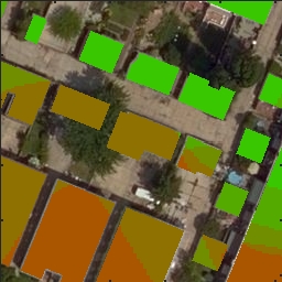
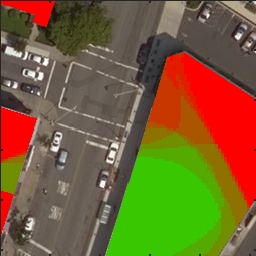
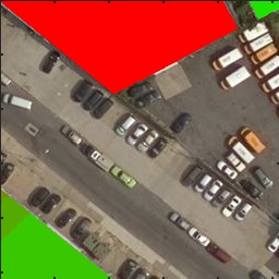
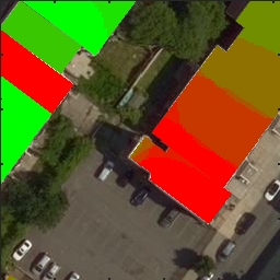
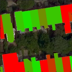
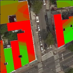
remote
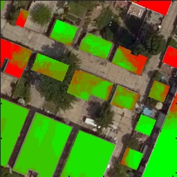
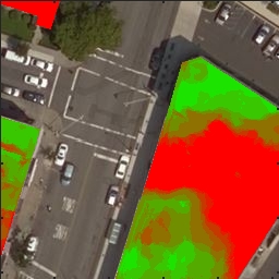
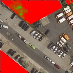
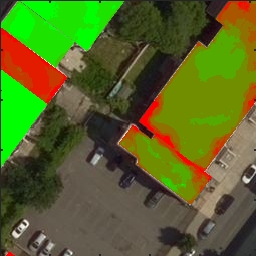
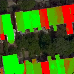
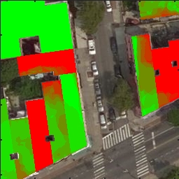
unified (adaptive)

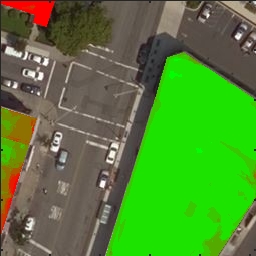
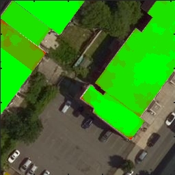
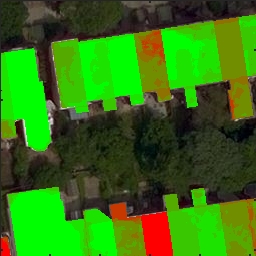
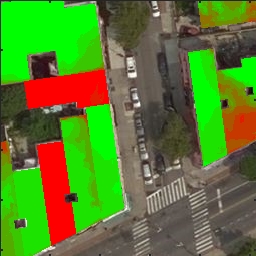
Figure 6: Sample results for identifying building function. From top to bottom, we visualize top-k images for the proximate, remote, and unified (adaptive) methods, respectively. Each pixel is color coded on a scale from green to red by the rank of the correct class in the posterior distribution, where bright green is the best (rank one).

ground truth
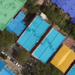
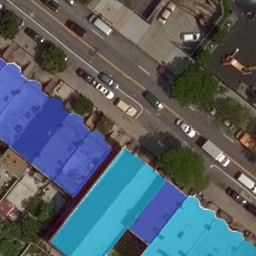
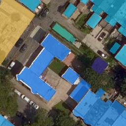
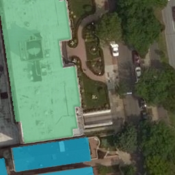
unified (ad.)

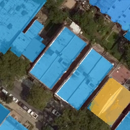
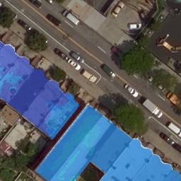
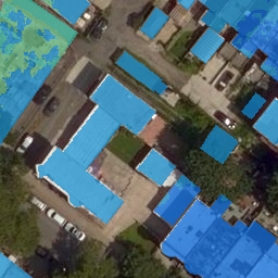
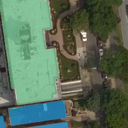
Figure 7: Sample results for estimating building age: (top) ground truth and (bottom) unified (adaptive).

Classifying Land Use.

We consider the task of identifying a parcel of land’s primary land use. This task is considered especially challenging from an overhead only perspective, with recent work simplifying the task by considering only three classes [28]. We report top-1 accuracy for land use classification using the Brooklyn test set in Table 1 and on Queens in Table 3. Similarly we report mIOU for Brooklyn and Queens in Table 2 and Table 4, respectively. Our results support the notion that this task is extremely difficult. However, our approach, unified (adaptive), is significantly better than all baselines, including an overhead image only approach (remote). Qualitative results for this task are shown in Figure 5.

Identifying Building Function.

We consider the task of making a functional map of buildings. To our knowledge, our work is the first to explore this. For example, in Figure 2, it becomes considerably easier to identify that the building in the overhead image is a fire station when shown two nearby ground-level images. We report performance metrics for this task in Table 1 and Table 3 for accuracy, and Table 2 and Table 4 for mIOU. Qualitative results are shown in Figure 6. Given the challenging nature of this task, we visualize results as a top-k image, where each pixel is colored from green (best) to red, by the rank of the correct class in the posterior distribution. Our approach produces labelings much more consistent with the ground truth.

Estimating Building Age.

Finally, we consider the task of estimating the year a building was constructed. Intuitively, this is an extremely difficult task from an overhead image only viewpoint, but is also non-trivial from a ground-level view. We report accuracy and mIOU metrics for this experiment in Table 1 and Table 2 for the Brooklyn region and Table 3 and in Table 4 for Queens. Our approach significantly outperforms the baselines. Example qualitative results are shown in Figure 7.

5.5 Does Known Orientation Help?

In the evaluation above, we constructed the ground-level feature map (Section 4.2) using features from geo-oriented panorama cutouts. The cutout images were extracted in the cardinal directions and their features stacked in a fixed order. To better understand the value of the ground-level feature map, we investigated how knowing the orientation of the ground-level images affects accuracy. We repeated the land use classification experiment on Brooklyn using our uniform (adaptive) approach (retraining the network), but randomly circular-shifted the set of images prior to feature extraction. Note that orientation is not completely random, because doing so would have required regenerating cutouts. We observe a significant performance drop from $77.40\%$ to $72.61\%$ in top-1 accuracy, about $3\%$ higher than using the overhead image only method. This experiment shows that knowing the orientation of the ground-level images is critical for achieving the best performance, but that including the ground-level images without knowing the orientation can still be useful.

6 Conclusion

We proposed a novel neural network architecture for estimating geospatial functions and evaluated it in the context of fine-grained understanding of an urban area. Our network fuses overhead and ground-level images and gives more accurate predictions than if either modality had been used in isolation. Specifically, our approach is better at resolving spatial boundaries than if only ground-level images were used and is better at estimating features that are difficult to determine from a purely overhead perspective. A key feature of our architecture is that it is end-to-end trainable, meaning that it can learn to extract the optimal features, for any appropriate loss function, from the raw pixels of all images, as well as parameters used to control the fusion process. While we demonstrated its use with ground-level images, our architecture is general and could be used with a wide variety of sparsely distributed measurements, including geotagged tweets, video, and audio.

Acknowledgments

We gratefully acknowledge the support of NSF CAREER grants IIS-1553116 (Jacobs) and IIS-1253549 (Crandall), a Google Faculty Research Award (Jacobs), and an equipment donation from IBM to the University of Kentucky Center for Computational Sciences.

Supplemental Material :
A Unified Model for Near and Remote Sensing

This document contains additional details and experiments related to our methods.

1 Brooklyn and Queens Dataset

Figure S1 shows the spatial coverage of the Brooklyn and Queens regions in our dataset. Figure S2 visualizes the label distributions for the Brooklyn and Queens test sets. Compared to Brooklyn, Queens has significantly different label occurrence. For example, for land use classification, Brooklyn has more “Public Buildings”, while Queens has more “Open Space/Recreation”.

2 Adaptive Bandwidth Visualization

In Figure S3 we visualize the estimated kernel bandwidth parameters, computed using our unified (adaptive) method for the task of land use classification, as a map for the Brooklyn and Queens regions. For each location, we display the mean of the diagonal entries of the kernel bandwidth matrix, $\Sigma$. These results show that the adaptive method is adjusting based on the underlying terrain.

3 Semantic Segmentation Results

Figure S4 shows confusion matrices for all three labeling tasks we consider (land use, age, function), each computed using the unified (adaptive) approach, for the Brooklyn test set. For building function estimation, we aggregate the 206 building classes into 30 higher-level classes. Classes are merged according to a hierarchy outlined by the New York City Department of City Planning in the PLUTO dataset. Despite the challenging nature of these tasks, our method seems to make sensible mistakes. For example, for the task of estimating building age, nearby decades are most often confused.

We report performance, top-1 accuracy and mean region intersection over union (mIOU), for building function estimation after aggregating the classes. For unified (adaptive), on the Brooklyn test set, top-1 accuracy increases to $61.08\%$ and mIOU increases to $30.40\%$. Similarly for Queens, top-1 accuracy increases to $52.01\%$ and mIOU increases to $14.99\%$.

In our experiments, we considered the $N=20$ closest ground-level images, chosen empirically based on available computational resources. Theoretically, there is no downside to including as many ground-level images as possible. However, we explored at what point performance might saturate. We performed this experiment for land use classification, using our unified (adaptive) approach, varying $N$ in increments of 5 up to 25, and found that performance saturated at $N=15$, but this was just one dataset/task. Figure S5 visualizes the results of this experiment using top-1 accuracy.

For each labeling task, we show additional semantic labeling results in Figure S6.

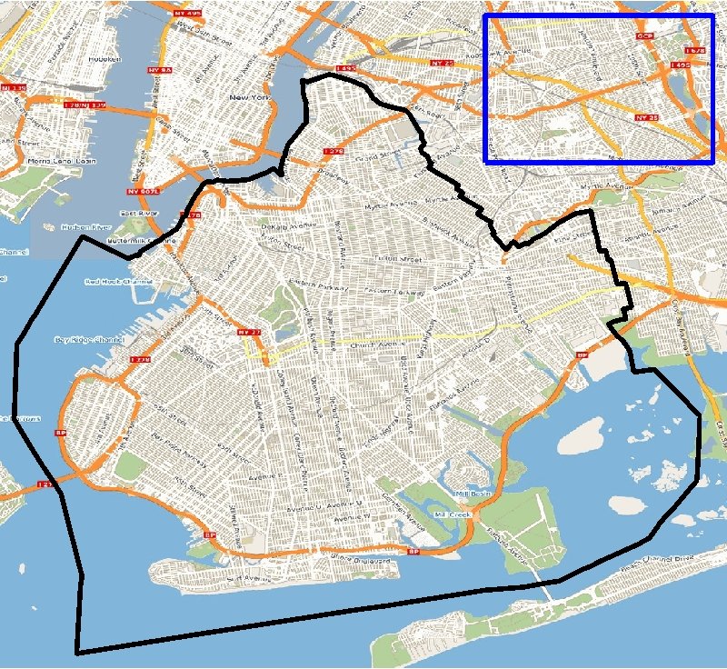
Figure S1: A coverage map for the Brooklyn (black) and Queens (blue) regions in our dataset.

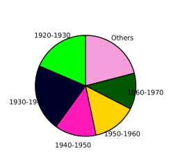
(a) Age

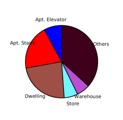
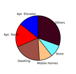
(b) Function

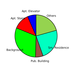
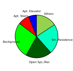
(c) Land Use

Figure S2: Distribution of labels for the Brooklyn (left) and Queens (right) test sets.

(a) Brooklyn

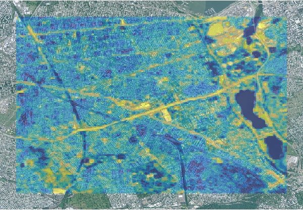
(b) Queens

Figure S3: Adaptive kernel bandwidth estimation. For each location we show the mean of the estimated optimal kernel bandwidth parameters, for the task of land use classification, computed using the unified (adaptive) method.

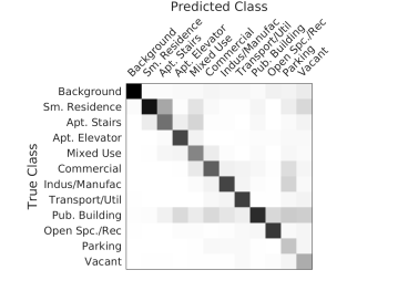
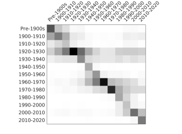
Figure S4: Confusion matrices for classifying land use (left), estimating building age (middle), and identifying building function (right). These results were computed using our unified (adaptive) approach for the Brooklyn test region.

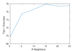
Figure S5: Varying the number of nearby ground-level images (land use classification). Each point corresponds to an instance of our unified (adaptive) method, except $N=0$ which reflects the performance of the remote baseline.

ground truth
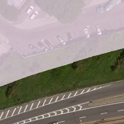
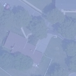
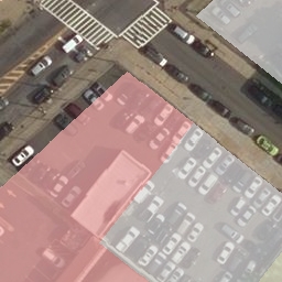
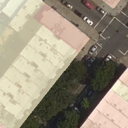
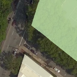
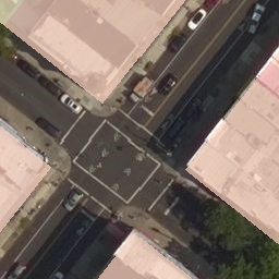
unified (adaptive)

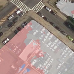
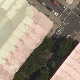
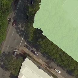
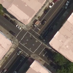
ground truth
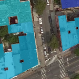
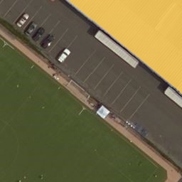
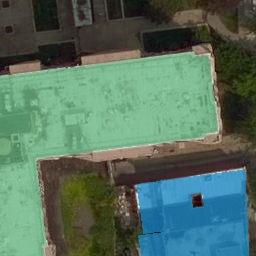
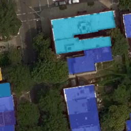
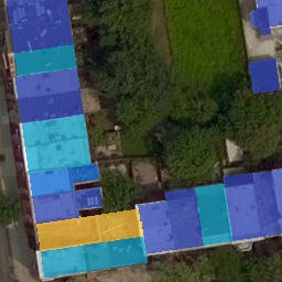
unified (adaptive)

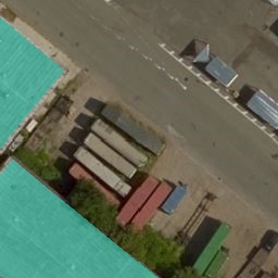
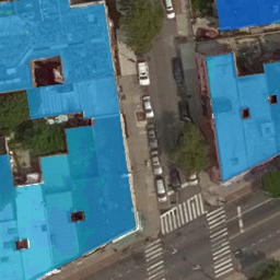
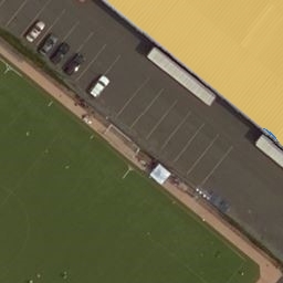
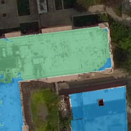
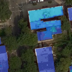
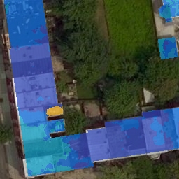
ground truth
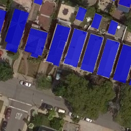
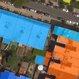
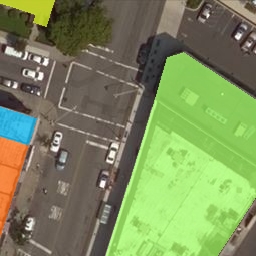
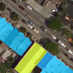
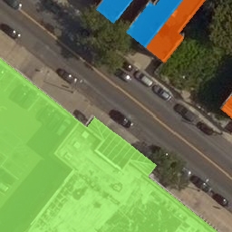
unified (adaptive)

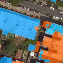
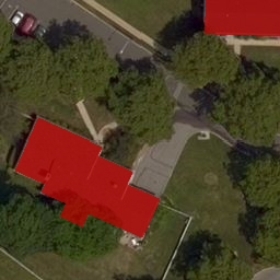
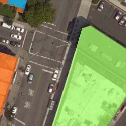
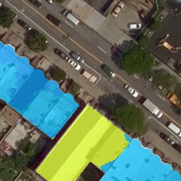
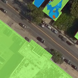
Figure S6: Additional semantic labeling results for classifying land use (top), estimating build age (middle) and identifying building function (bottom).

References

- [1] M. Abadi, A. Agarwal, P. Barham, E. Brevdo, Z. Chen, C. Citro, G. S. Corrado, A. Davis, J. Dean, M. Devin, et al. Tensorflow: Large-scale machine learning on heterogeneous distributed systems. arXiv preprint arXiv:1603.04467, 2016.
- [2] S. M. Arietta, A. A. Efros, R. Ramamoorthi, and M. Agrawala. City forensics: Using visual elements to predict non-visual city attributes. IEEE Transactions on Visualization and Computer Graphics, 20(12):2624–2633, 2014.
- [3] A. Bansal, X. Chen, B. Russell, A. G. Ramanan, et al. Pixelnet: Representation of the pixels, by the pixels, and for the pixels. arXiv preprint arXiv:1702.06506, 2017.
- [4] A. Dubey, N. Naik, D. Parikh, R. Raskar, and C. A. Hidalgo. Deep learning the city: Quantifying urban perception at a global scale. In European Conference on Computer Vision, 2016.
- [5] R. Fedorov, P. Fraternali, C. Pasini, and M. Tagliasacchi. SnowWatch: snow monitoring through acquisition and analysis of user-generated content. arXiv:1507.08958, 2015.
- [6] R. Fedorov, P. Fraternali, and M. Tagliasacchi. Snow phenomena modeling through online public media. In IEEE International Conference on Image Processing, 2014.
- [7] N. Ghouaiel and S. Lefèvre. Coupling ground-level panoramas and aerial imagery for change detection. Geo-spatial Information Science, 19(3):222–232, 2016.
- [8] D. Glasner, P. Fua, T. Zickler, and L. Zelnik-Manor. Hot or not: Exploring correlations between appearance and temperature. In IEEE International Conference on Computer Vision, 2015.
- [9] B. Hariharan, P. Arbeláez, R. Girshick, and J. Malik. Hypercolumns for object segmentation and fine-grained localization. In IEEE Conference on Computer Vision and Pattern Recognition, 2015.
- [10] S. Ioffe and C. Szegedy. Batch normalization: Accelerating deep network training by reducing internal covariate shift. In International Conference on Machine Learning, 2015.
- [11] N. Jacobs, S. Workman, and R. Souvenir. Cloudmaps from Static Ground-View Video. Image and Vision Computing (IVC), 52:154–166, 2016.
- [12] A. Khosla, B. An, J. J. Lim, and A. Torralba. Looking beyond the visible scene. In IEEE Conference on Computer Vision and Pattern Recognition, 2014.
- [13] D. Kingma and J. Ba. Adam: A method for stochastic optimization. In International Conference on Learning Representations, 2014.
- [14] S. Lee, H. Zhang, and D. J. Crandall. Predicting geo-informative attributes in large-scale image collections using convolutional neural networks. In IEEE Winter Conference on Applications of Computer Vision, 2014.
- [15] D. Leung and S. Newsam. Proximate sensing: Inferring what-is-where from georeferenced photo collections. In IEEE Conference on Computer Vision and Pattern Recognition, 2010.
- [16] Y. Li, J. Huang, and J. Luo. Using user generated online photos to estimate and monitor air pollution in major cities. In ACM International Conference on Internet Multimedia Computing and Service, 2015.
- [17] T.-Y. Lin, S. Belongie, and J. Hays. Cross-view image geolocalization. In IEEE Conference on Computer Vision and Pattern Recognition, 2013.
- [18] T.-Y. Lin, Y. Cui, S. Belongie, and J. Hays. Learning deep representations for ground-to-aerial geolocalization. In IEEE Conference on Computer Vision and Pattern Recognition, 2015.
- [19] J. Luo, J. Yu, D. Joshi, and W. Hao. Event recognition: viewing the world with a third eye. In ACM International Conference on Multimedia, 2008.
- [20] G. Máttyus, S. Wang, S. Fidler, and R. Urtasun. Hd maps: Fine-grained road segmentation by parsing ground and aerial images. In IEEE Conference on Computer Vision and Pattern Recognition, 2016.
- [21] C. Murdock, N. Jacobs, and R. Pless. Webcam2satellite: Estimating cloud maps from webcam imagery. In IEEE Workshop on Applications of Computer Vision, 2013.
- [22] C. Murdock, N. Jacobs, and R. Pless. Building dynamic cloud maps from the ground up. In IEEE International Conference on Computer Vision, 2015.
- [23] L. Porzi, S. Rota Bulò, B. Lepri, and E. Ricci. Predicting and understanding urban perception with convolutional neural networks. In ACM International Conference on Multimedia, 2015.
- [24] O. Rozenstein and A. Karnieli. Comparison of methods for land-use classification incorporating remote sensing and gis inputs. Applied Geography, 31(2):533–544, 2011.
- [25] K. Simonyan and A. Zisserman. Very deep convolutional networks for large-scale image recognition. In International Conference on Learning Representations, 2015.
- [26] K. Tang, M. Paluri, L. Fei-Fei, R. Fergus, and L. Bourdev. Improving image classification with location context. In IEEE International Conference on Computer Vision, 2015.
- [27] J. Wang, M. Korayem, S. Blanco, and D. Crandall. Tracking natural events through social media and computer vision. In ACM International Conference on Multimedia, 2016.
- [28] S. Wang, M. Bai, G. Mattyus, H. Chu, W. Luo, B. Yang, J. Liang, J. Cheverie, S. Fidler, and R. Urtasun. Torontocity: Seeing the world with a million eyes. arXiv preprint arXiv:1612.00423, 2016.
- [29] J. D. Wegner, S. Branson, D. Hall, K. Schindler, and P. Perona. Cataloging public objects using aerial and street-level images-urban trees. In IEEE Conference on Computer Vision and Pattern Recognition, 2016.
- [30] S. Workman and N. Jacobs. On the location dependence of convolutional neural network features. In IEEE/ISPRS Workshop: EARTHVISION: Looking From Above: When Earth Observation Meets Vision, 2015.
- [31] S. Workman, R. Souvenir, and N. Jacobs. Wide-area image geolocalization with aerial reference imagery. In IEEE International Conference on Computer Vision, 2015.
- [32] S. Workman, R. Souvenir, and N. Jacobs. Understanding and mapping natural beauty. In IEEE International Conference on Computer Vision, 2017.
- [33] L. Xie and S. Newsam. Im2map: deriving maps from georeferenced community contributed photo collections. In ACM SIGMM International Workshop on Social Media, 2011.
- [34] M. Xie, N. Jean, M. Burke, D. Lobell, and S. Ermon. Transfer learning from deep features for remote sensing and poverty mapping. In AAAI Conference on Artificial Intelligence, 2015.
- [35] M. Zhai, Z. Bessinger, S. Workman, and N. Jacobs. Predicting ground-level scene layout from aerial imagery. In IEEE Conference on Computer Vision and Pattern Recognition, 2017.
- [36] B. Zhou, A. Lapedriza, A. Khosla, A. Oliva, and A. Torralba. Places: A 10 million image database for scene recognition. IEEE Transactions on Pattern Analysis and Machine Intelligence, PP(99), 2017.
- [37] B. Zhou, L. Liu, A. Oliva, and A. Torralba. Recognizing city identity via attribute analysis of geo-tagged images. In European Conference on Computer Vision, 2014.
- [38] Y. Zhu and S. Newsam. Land use classification using convolutional neural networks applied to ground-level images. In ACM SIGSPATIAL International Conference on Advances in Geographic Information Systems, 2015.