Stable and unstable roots of ion temperature gradient driven mode using curvature modified plasma dispersion functions

Abstract

Basic, local kinetic theory of ion temperature gradient driven (ITG) mode, with adiabatic electrons is reconsidered. Standard unstable, purely oscillating as well as damped solutions of the local dispersion relation are obtained using a bracketing technique that uses the argument principle. This method requires computing the plasma dielectric function and its derivatives, which are implemented here using modified plasma dispersion functions with curvature and their derivatives, and allows bracketing/following the zeros of the plasma dielectric function which corresponds to different roots of the ITG dispersion relation. We provide an open source implementation of the derivatives of modified plasma dispersion functions with curvature, which are used in this formulation. Studying the local ITG dispersion, we find that near the threshold of instability the unstable branch is rather asymmetric with oscillating solutions towards lower wave numbers (i.e. drift waves), and damped solutions toward higher wave numbers. This suggests a process akin to inverse cascade by coupling to the oscillating branch towards lower wave numbers may play a role in the nonlinear evolution of the ITG, near the instability threshold. Also, using the algorithm, the linear wave diffusion is estimated for the marginally stable ITG mode.

I Introduction

I.1 Background

Ion temperature gradient driven (ITG) mode was studied in great detail over the years in light of its relevance for transport in magnetized fusion devices(Coppi et al., 1967; Wendell Horton et al., 1981; Lee and Diamond, 1986). A basic formulation of the kinetic ITG that has been studied in the past is a local, electrostatic description based on the gyrokinetic equation(Catto, 1978; Frieman and Chen, 1982; Hahm, 1988) for ions, with adiabatic electrons, where the linear problem boils down to finding the roots of the plasma dielectric function $\varepsilon\left(\omega,\mathbf{k}\right)$ numerically.

Kinetic waves in electrostatic plasmas in general, can be described using the so-called plasma dispersion function (Fried and Conte, 1961). The cylindrical ITG mode for instance, can be formulated completely in terms of plasma dispersion functions(Mattor and Diamond, 1989). The advantage of such a formulation is that, the plasma dispersion function is linked to the complex error function and there exists efficient methods for its computation(Gautschi, 1970).

Recently, a similar, numerically efficient reformulation of local ITG in terms of curvature modified plasma dispersion functions was proposed (Gürcan, 2014), which is equivalent to the formulation in Refs. (Kim et al., 1994; Kuroda et al., 1998). These functions, dubbed $I_{nm}\left(\zeta_{\alpha},\zeta_{\beta},b\right)$, and defined for $Im\left[\zeta_{\alpha}\right]>0$ as:

$$I_{nm}\left(\zeta_{\alpha},\zeta_{\beta},b\right)\equiv$$

$$\frac{2}{\sqrt{\pi}}\int_{0}^{\infty}dx_{\perp}\int_{-\infty}^{\infty}dx_{\parallel}\frac{x_{\perp}^{n}x_{\parallel}^{m}J_{0}^{2}\left(\sqrt{2b}x_{\perp}\right)e^{-x^{2}}}{\left(x_{\parallel}^{2}+\frac{x_{\perp}^{2}}{2}+\zeta_{\alpha}-\zeta_{\beta}x_{\parallel}\right)}\;\text{,}$$ (1)

can be written as a 1D integral of a combination of plasma dispersion functions, instead of the two dimensional integral shown above. Note that, since these functions have been formulated with built-in analytical continuation, a dispersion relation, written with these functions, can be used to describe oscillating and damped solutions as well as unstable ones.

In this paper, we extend the space of curvature modified plasma dispersion functions by including their derivatives [i.e. $J_{nm}\left(\zeta_{\alpha},\zeta_{\beta},b\right)\equiv-\frac{\partial}{\partial\zeta_{\alpha}}I_{nm}\left(\zeta_{\alpha},\zeta_{\beta},b\right)$], defined as

$$J_{nm}\left(\zeta_{\alpha},\zeta_{\beta},b\right)\equiv$$

$$\frac{2}{\sqrt{\pi}}\int_{0}^{\infty}dx_{\perp}\int_{-\infty}^{\infty}dx_{\parallel}\frac{x_{\perp}^{n}x_{\parallel}^{m}J_{0}^{2}\left(\sqrt{2b}x_{\perp}\right)e^{-x^{2}}}{\left(x_{\parallel}^{2}+\frac{x_{\perp}^{2}}{2}+\zeta_{\alpha}-\zeta_{\beta}x_{\parallel}\right)^{2}}\;\text{,}$$ (2)

and use these functions in order to compute the derivatives of the plasma dielectric function $\varepsilon\left(\omega,\mathbf{k}\right)$ with respect to the angular frequency $\omega$. This allows the use of a root finding alogrithm based on the argument principle as discussed for instance in Ref.(Johnson and Tucker, 2009) (similar to the method used in the quasi-linear solver QualiKiz(Bourdelle et al., 2007) and detailed in Ref. (Davies, 1986)), which allows us to obtain both unstable and stable roots.

Notice that in most cases, the stable roots are considered to have a negligible effect on transport and are therefore ignored. However, from a simple quasi-linear theory (QLT) point of view, this is clearly not permissible, since as the nonlinear interactions appear, so does the transfer of energy to stable or damped modes. However, from a renormalized QLT perspective -à la Balescu (Balescu, 2005), which is actually how the use of QLT to estimate transport is really justified- it is unclear whether one may use a single dominant (but renormalized) mode, or one still has to consider a coupling of a number of stable and unstable modes (even if each one of those modes are modified due to nonlinear effects, via mechanisms such as eddy damping). This may be crucial in particular if after renormalization, the most unstable (or the least damped) mode for a given wave-vector becomes subdominant to a previously subdominant mode.

The rest of the paper is organized as follows. In section II, the local ITG dispersion relation is recalled using curvature modified plasma dispersion functions, $I_{nm}$’s. Then, in subsection b), derivatives of the curvature modified dispersion functions are defined as $J_{nm}$’s, and the derivative of the plasma dielectric tensor is written in terms of $J_{nm}$’s. In Section III, methods and examples, first an efficient and accurate method for finding and tracing the roots of the dispersion relation is introduced in subsection a), and then an example of linear wave diffusion of an unstable mode into linearly stable region is considered and the diffusion coefficient is estimated. Section IV is results and conclusion.

II Formulation

II.1 Linear Dispersion Using $I_{nm}$’s:

A basic description of local kinetic ITG in the electrostatic limit, with adiabatic electrons is based on the gyrokinetic equation (Frieman and Chen, 1982; Lee, 1983; Hahm, 1988) for the non-adiabatic part of the fluctuating distribution function for the ions:

$$\frac{\partial}{\partial t}\delta g+ \left[v_{\parallel}\frac{\mathbf{B}^{*}}{B}+\frac{\mu}{eB}\hat{\mathbf{b}}\times\nabla B\right]\cdot\nabla\delta g=\frac{e}{T_{i}}F_{0}\frac{\partial}{\partial t}\left\langle\delta\Phi\right\rangle-F_{0}\frac{\hat{\mathbf{b}}}{B}\times\nabla\left\langle\delta\Phi\right\rangle\cdot\left[\frac{1}{n}\nabla n+\left(\frac{E}{T}-\frac{3}{2}\right)\frac{1}{T}\nabla T\right]\;\text{.}$$ (3)

This is then complemented by the quasi-neutrality relation ($n_{e}=n_{i}$), with adiabatic electrons:

$$\frac{e}{T_{e}}\Phi=-\frac{e\Phi}{T_{i}}+\int J_{0}\delta gd^{3}v\;\text{.}$$ (4)

Taking the Laplace-Fourier transform of (3) in the form $\delta g_{\mathbf{k},\omega}\left(\mathbf{v}\right)=\int e^{-i\omega t+i\mathbf{k}\cdot\mathbf{x}}\delta g\left(\mathbf{x},\mathbf{v},t\right)$ and solving for $\delta g_{\mathbf{k},\omega}$ and substituting the result into (4), we obtain the dispersion relation in the form:

$$\varepsilon\left(\omega,\mathbf{k}\right)\equiv 1+\frac{1}{\tau}-\left[\frac{1}{\sqrt{2\pi}v_{ti}^{3}}\int\frac{\left(\omega-\omega_{*Ti}\left(v\right)\right)J_{0}\left(\frac{v_{\perp}k_{\perp}}{\Omega_{i}}\right)^{2}}{\left(\omega-v_{\parallel}k_{\parallel}-\omega_{Di}\frac{1}{2}\left(\frac{v_{\parallel}^{2}}{v_{ti}^{2}}+\frac{v_{\perp}^{2}}{2v_{ti}^{2}}\right)\right)}e^{-\frac{v^{2}}{2v_{ti}^{2}}}v_{\perp}dv_{\perp}dv_{\parallel}\right]=0\;\text{,}$$ (5)

where $\varepsilon\left(\omega,\mathbf{k}\right)$ is the plasma dielectric function,

$$\omega_{*Ti}\left(v\right)\equiv\omega_{*i}\left[1+\left(\frac{v^{2}}{2v_{ti}^{2}}-\frac{3}{2}\right)\eta_{i}\right]\;\mbox{,}$$

and $\omega_{Di}=2\frac{L_{n}}{R}\omega_{*i}$. Using $\omega/\left|k_{y}\right|\rightarrow\omega$, and $\omega_{D}/\left|k_{y}\right|\rightarrow\omega_{D}$, the dispersion relation (5) can be written as:

$$\varepsilon\left(\omega,\mathbf{k}\right)\equiv 1+\frac{1}{\tau}+\frac{1}{\omega_{Di}}\bigg{(}I_{10}\left[\omega+\left(1-\frac{3}{2}\eta_{i}\right)\right]$$

$$+\left(I_{30}+I_{12}\right)\eta_{i}\bigg{)}=0$$ (6)

where $I_{nm}\equiv I_{nm}\left(-\frac{\omega}{\omega_{Di}},-\frac{\sqrt{2}k_{\parallel}}{\omega_{Di}k_{y}},b\right)$. The advantage of this particular form is that the explicit scaling of $\omega$ with $k_{y}$ is removed, so that we can define a region in $\omega$ space to search for roots, and do not need to scale it with $k_{y}$.

As discussed in detail in Ref. Gürcan, 2014, the $I_{nm}$’s can be written as a single integral:

$$I_{nm}\left(\zeta_{\alpha},\zeta_{\beta},b\right)=$$

$$\int_{0}^{\infty}s^{\frac{n-1}{2}}G_{m}\left(z_{1}\left(s\right),z_{2}\left(s\right)\right)J_{0}\left(\sqrt{2bs}\right)^{2}e^{-s}ds\;\mbox{,}$$

$$\quad(Im\left[\zeta_{\alpha}\right]>0)$$

using the straightforward multi-variable generalization of the standard plasma dispersion function:

$$G_{m}\left(z_{1},z_{2},\cdots,z_{n}\right)\equiv\frac{1}{\sqrt{\pi}}\int_{-\infty}^{\infty}\frac{x^{m}e^{-x^{2}}}{\prod_{i=1}^{n}\left(x-z_{i}\right)}dx$$ (7)

with

$$z_{1,2}\left(s\right)=\frac{1}{2}\left(\zeta_{\beta}\pm\sqrt{\zeta_{\beta}^{2}-2\left(s+2\zeta_{\alpha}\right)}\right)\;\mbox{.}$$ (8)

Note that, using Eqns. 4 and 6 of Ref. Gürcan, 2014, we can write the $G_{m}\left(z_{1},z_{2}\right)$ in terms of the standard plasma dispersion function as:

$$G_{m}\left(z_{1},z_{2}\right) =\frac{1}{\sqrt{\pi}\left(z_{1}-z_{2}\right)}\bigg{[}z_{1}^{m}Z_{0}\left(z_{1}\right)-z_{2}^{m}Z_{0}\left(z_{2}\right)$$

$$+\sum_{k=2}^{m}\left(z_{1}^{k-1}-z_{2}^{k-1}\right)\Gamma\left(\frac{m-k+1}{2}\right)\bigg{]}\;,$$ (9)

which was then implemented using a 16 coefficient Weideman method (Weideman, 1994), in the form of an open source fortran library [http://github.com/gurcani/zpdgen] with a python interface.

As discussed in Refs. Kim et al., 1994 and Kuroda et al., 1998. In addition to the integral in (6), the analytical continuation requires adding a residue contribution, which can be computed as

$$\Delta I_{nm}\left(\zeta_{\alpha},\zeta_{\beta},b\right)=-i\sqrt{\pi}2^{\frac{\left(n+3\right)}{2}}w^{\frac{n}{2}}\int_{-1}^{1}d\mu \left(1-\mu^{2}\right)^{\frac{\left(n-1\right)}{2}}\left(\mu\sqrt{w}+\frac{\zeta_{\beta}}{2}\right)^{m}$$

$$J_{0}^{2}\left(2\sqrt{b\left(1-\mu^{2}\right)w}\right)e^{-2\left(1-\mu^{2}\right)w-\left(\mu\sqrt{w}+\frac{\zeta_{\beta}}{2}\right)^{2}}\times\begin{cases}0&\zeta_{\alpha i}>0\quad\mbox{or }w_{r}<0\\ \frac{1}{2}&\zeta_{\alpha i}=0\quad\mbox{and }w_{r}>0\\ 1&\zeta_{\alpha i}<0\quad\mbox{and }w_{r}>0\end{cases}$$

where $w=\frac{\zeta_{\beta}^{2}}{4}-\zeta_{\alpha}$ and $\zeta_{\alpha i}=\text{Im}\left(\zeta_{\alpha}\right)$ and $w_{r}=\text{Re}\left[w\right]$. With this, $I_{nm}=I_{nm}^{{}^{\prime}}+\Delta I_{nm}$ [where $I_{nm}^{{}^{\prime}}$ is the integral in (6)] is defined everywhere on the complex plane.

II.2 Derivatives of $I_{nm}$’s

Similarly the derivatives as defined by the relation

$$J_{nm}\left(\zeta_{\alpha},\zeta_{\beta},b\right)\equiv-\frac{\partial}{\partial\zeta_{\alpha}}I_{nm}\left(\zeta_{\alpha},\zeta_{\beta},b\right)$$

can be written using

$$J_{nm}\left(\zeta_{\alpha},\zeta_{\beta},b\right)=$$

$$\int_{0}^{\infty}ds\left[s^{\frac{n-1}{2}}G_{m}\left(z_{1},z_{2},z_{1},z_{2}\right)J_{0}\left(\sqrt{2bs}\right)^{2}e^{-s}\right]\;\mbox{,}$$

$$\quad(Im\left[\zeta_{\alpha}\right]>0)$$ (10)

with repeating variables $z_{1}=z_{1}\left(s\right)$ and $z_{2}=z_{2}\left(s\right)$ as given in (8). Since the $\zeta_{\alpha}$ dependence is through $z_{1}$ and $z_{2}$, we can use (8) to compute the derivatives , acting $\frac{d}{d\zeta_{\alpha}}=\frac{1}{\left(z_{1}-z_{2}\right)}\left(\frac{d}{dz_{2}}-\frac{d}{dz_{1}}\right)$ on (9), in order to obtain:

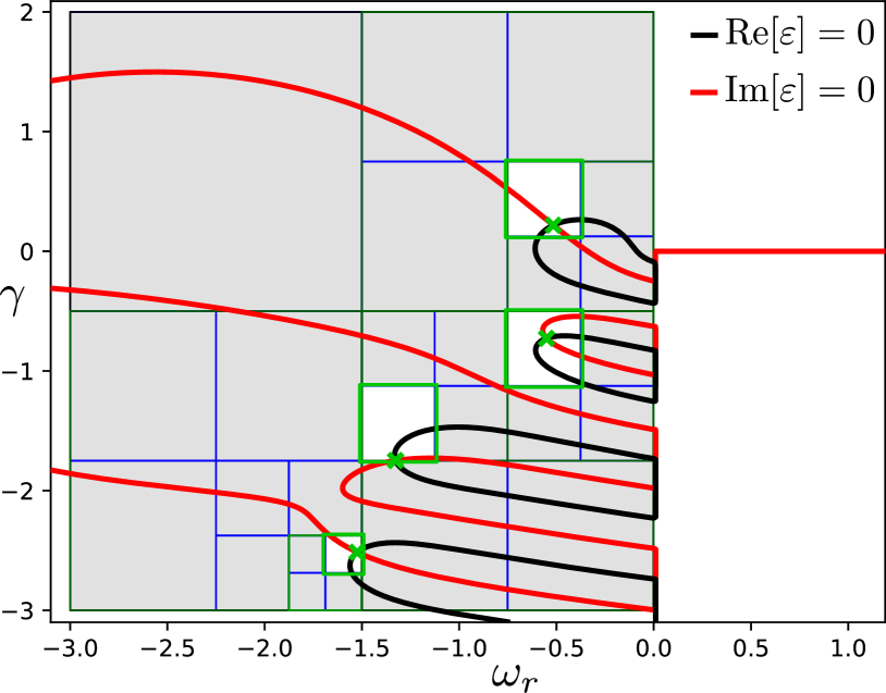
Figure 1: The way the bracketing algorithm isolates the roots of the plasma dielectric function (6) to a desired rectangle size. Shaded rectangles contain no roots and so are immediately abandoned. The roots, which are depicted by x’s are found using a least square optimization, where the midpoint of the final rectangle is used as the initial guess, and the rectangle itself is used as a boundary. The case that is shown here is $k_{y}=0.8$, which is usually used as the reference $k_{y}$.

$$G_{m}\left(z_{1},z_{2},z_{1},z_{2}\right) =-\frac{d}{d\zeta_{\alpha}}G_{m}\left(z_{1},z_{2}\right)=\frac{1}{\left(z_{1}-z_{2}\right)^{2}}\bigg{\{}\frac{1}{\sqrt{\pi}}\sum_{k=2}^{m}\left[\left(k-1\right)\left(z_{1}^{k-2}+z_{2}^{k-2}\right)-\frac{2\left(z_{1}^{k-1}-z_{2}^{k-1}\right)}{\left(z_{1}-z_{2}\right)}\right]\Gamma\left(\frac{m-k+1}{2}\right)$$

$$-2\left(z_{1}^{m}+z_{2}^{m}\right)+Z_{0}\left(z_{1}\right)z_{1}^{m-1}\left(m-2z_{1}^{2}-\frac{2z_{1}}{\left(z_{1}-z_{2}\right)}\right)+Z_{0}\left(z_{2}\right)z_{2}^{m-1}\left(m-2z_{2}^{2}+\frac{2z_{2}}{\left(z_{1}-z_{2}\right)}\right)\bigg{\}}\text{\;.}$$ (11)

We also have to compute the derivatives of the residue contribution $\Delta I_{nm}$, which we dub $\Delta J_{nm}$ (note that, this is derivative of the residue and not the residue of the derivative), and can be written as:

$$\Delta J_{nm}= -i\sqrt{\pi}2^{\frac{n+3}{2}}\int_{-1}^{1}\bigg{\{}\left(\frac{n}{2w}+\frac{\mu m}{2\mu w+\sqrt{w}\zeta_{\beta}}-2+\mu^{2}-\frac{\zeta_{\beta}}{2}\frac{\mu}{\sqrt{w}}\right)J_{0}^{2}\left(2\sqrt{b\left(1-\mu^{2}\right)w}\right)$$

$$-2\sqrt{\frac{b\left(1-\mu^{2}\right)}{w}}J_{0}\left(2\sqrt{b\left(1-\mu^{2}\right)w}\right)J_{1}\left(2\sqrt{b\left(1-\mu^{2}\right)w}\right)\bigg{\}}$$

$$w^{n/2}\left(1-\mu^{2}\right)^{\frac{n-1}{2}}\left(\mu\sqrt{w}+\frac{\zeta_{\beta}}{2}\right)^{m}e^{-2\left(1-\mu^{2}\right)w-\left(\mu\sqrt{w}+\frac{\zeta_{\beta}}{2}\right)^{2}}d\mu\times\begin{cases}0&\zeta_{\alpha i}>0\quad\mbox{or }w_{r}<0\\ \frac{1}{2}&\zeta_{\alpha i}=0\quad\mbox{and }w_{r}>0\\ 1&\zeta_{\alpha i}<0\quad\mbox{and }w_{r}>0\end{cases}$$ (12)

where we used the definition $\Delta J_{nm}=-\frac{d}{d\zeta_{\alpha}}\Delta I_{nm}=\frac{d}{dw}\Delta I_{nm}$. Finally, $J_{nm}=J_{nm}^{{}^{\prime}}+\Delta J_{nm}$ where $J_{nm}^{{}^{\prime}}$ is the integral given in (10) with (11).

Using these $J_{nm}$ functions, which denote derivatives of the curvature modified plasma dispersion functions with respect to the first variable, the derivative of the plasma dielectric function can be written as:

$$\frac{\partial}{\partial\omega}\varepsilon\left(\omega,\mathbf{k}\right)\equiv\frac{1}{\omega_{Di}}I_{10} +\frac{1}{\omega_{D}^{2}}\bigg{(}J_{10}\left[\omega+\left(1-\frac{3}{2}\eta_{i}\right)\right]$$

$$+\left(J_{30}+J_{12}\right)\eta_{i}\bigg{)}\;\text{.}$$ (13)

where $J_{nm}\equiv J_{nm}\left(-\frac{\omega}{\omega_{Di}},-\frac{\sqrt{2}k_{\parallel}}{\omega_{Di}k_{y}},b\right)$, and $\omega$ and $\omega_{D}$ are normalized to $\left|k_{y}\right|$ for convenience.

III Methods and Examples

III.1 Finding and tracking stable and unstable solutions

Fixing the values of plasma parameters such as $\eta_{i}$, $R/L_{n}$ and $\tau$, we can solve (6) for $\omega$, for a given $\mathbf{k}$. In practice we fix $k_{\parallel}$ and $k_{x}$ and consider $\omega$ as a function of $k_{y}$. While there are many different ways of achieving this numerically, we have developed a simple algorithm for bracketing, solving and then tracing each root of the solution. Generally we pick a reference $k_{y}$ value, where we think the roots are reasonably distinct (choosing this reference $k_{y}$ may require trial and error). Then we use an algorithm very similar to the one outlined in Ref. Johnson and Tucker, 2009 in order to bracket each solution as shown in Fig. 1, with an initial rectangle that covers only the $\omega_{r}<0$ part of the complex plane avoiding the line $\omega_{r}=0$, where there is a branch cut. In fact a desired number of roots (i.e. $N_{r}$) are specified so that the algoritm repeats itself with larger and larger rectangles (always avoiding the branch cut) until the desired number of roots fall within the rectangle. This gives us $N_{r}$ rectangles with a root in each one. Then, a basic least square optimization is used to locate the exact root within each rectangle. Note that a small buffer is added around the boundary of the rectangle in order to succeed in cases where the point falls exactly on the boundary of the rectangle (e.g. third root from above in Fig. 1).

When the $k_{y}$ is varied, a new rectangle is defined for each $N_{r}$ root, using the solutions from one of the previous steps (i.e. nearest $k_{y}$, for which $\omega$ have already been computed), with a predefined rectangle size (i.e. if $k_{y}$ resolution is high enough, the rectangle sizes can be very small and there are virtually no intersections), and the least square optimization is used again to find the new solutions in each rectangle. This allows us to trace curves in $\omega=\omega\left(k_{y}\right)$, which help distinguish different roots. Note that tracking $\omega$ as a function of $k_{y}$ instead of repeating the bracketing step each time, saves a huge amount of computation time. Such an approach would be useful also in quasilinear transport modelling geared towards speed(Bourdelle et al., 2007).

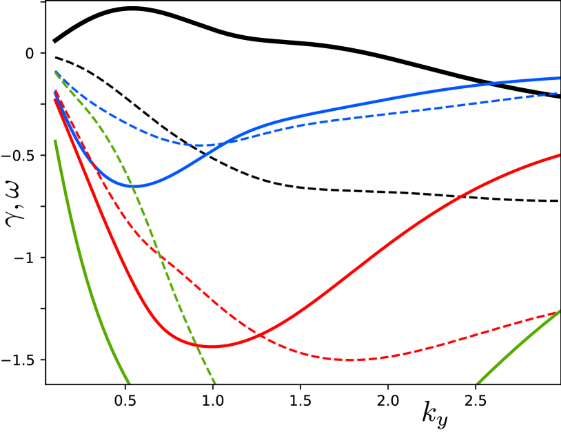
Figure 2: Growth rates $\gamma$ (solid lines), and frequencies $\omega$ (dashed lines) as functions of $k_{y}$, for the first four roots of the local, kinetic ITG dispersion relation as defined in (6), where each color denotes a seperate root. Note that around $k_{y}=2.5$, the second root becomes less damped than the unstable branch.

In any case, bracketing is necessary in order to isolate the different roots of (6). Since the algorithm relies on the argument principle

$$\oint_{C}\frac{\frac{\partial}{\partial\omega}\varepsilon\left(\omega,\mathbf{k}\right)}{\varepsilon\left(\omega,\mathbf{k}\right)}d\omega=2\pi i\left(N-P\right)$$

where $N$ and $P$ are the number of poles and zeros in the closed contour defined by$C$, we use (13) in order to compute the derivative of the plasma dielectric function analytically.

Figure 3: Growth rate $\gamma$ (solid line), and frequency $\omega$ (dashed lines) as functions of $k_{y}$, for the dominant root of the ITG dispersion relation near the threshold of instability (i.e. $\eta_{i}=0.68$). Note that the damped modes in this case, are strongly damped (i.e. $\gamma_{d}<-0.2$) as compared to the unstable mode.

Using this method, the growth (and damping) rates as well as frequencies for the reference shot studied in Ref. Kim et al., 1994 (i.e. $\eta_{i}=2.5$, $L_{n}/R=0.2$, $\tau=1.0$ and $k_{\parallel}=0.01$) is shown in Fig. 2. It is remarkable that for these parameters, around $k_{y}=2.5$, the second root becomes less damped than the unstable branch. Since trapped electron physics is ignored, the second root never actually becomes unstable.

Another interesting observation about the nature of the roots of this particular limit of the gyrokinetic equation, is that near the instability threshold (slightly above, or slightly below), one observes a region to the left (in $k_{y}$ space) of the linearly most unstable (or the least damped) mode, where the solution becomes a propagating wave in the electron diamagnetic direction (i.e. $\omega>0$) as seen in Fig. 3. This is the drift wave (DW) branch, that is modified due to the weak ion temperature gradient. This is not a surprise, since the equations considered in this paper should recover the drift wave limit as the ITG drive disappears.

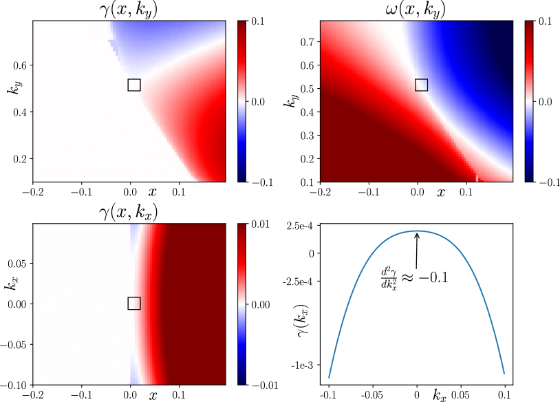
Figure 4: Profiles of a) the growth rate $\gamma_{k}$ as a function of position ($x$-axis) and $k_{y}$ (y-axis) at $k_{x}=0$, b) the real frequency as a function of position ($x$-axis) and $k_{y}$ (y-axis) at $k_{x}=0$, c) the growth rate $\gamma_{k}$ as a function of position ($x$-axis) and $k_{x}$ (y-axis) at $k_{y}=k_{yc}$, where $k_{yc}$ is the most unstable wavenumber at $x=k_{x}=0$, d) the growth rate $\gamma_{k}$ as a function of $k_{x}$ at $k_{y}=k_{yc}$ and $x=0$. The box shows the marginal point. As can be seen in a) and b), the growth rate $\gamma=0$ to the left of the marginal point (i.e. for which $\eta_{i}<\eta_{ic}$), where the frequency is positive (i.e. electron diamagnetic direction).

III.2 Example: Linear diffusion near marginality

For a given set of plasma parameters, $\eta_{i}$ determines the stability of the ITG mode. Considering $\eta_{i}$ as a function of $x$ , for instance of the form $\eta_{i}\left(x\right)=\eta_{ic}+\delta\eta_{i}\left[\frac{x-x_{0}}{x_{1}-x_{0}}\right]$, we can define a resonable description of an unstable region next to a stable region. The issue of turbulence spreading into the unstable region is a complex one and is out of the scope of the current paper. Here we discuss how a monochromatic wave, propagating mainly in the $y$ direction can diffuse in the radial direction due to $\partial^{2}\gamma_{k}/\partial k_{x}^{2}$ being finite and negative. Consider the evolution of the amplitude of ITG mode near its stability boundary. Close enough to the marginal stability, only a single mode will be linearly unstable. We can write the general two scale evolution equation for the amplitude of that mode in the form

$$\left(\partial_{t}+v_{gi}\partial_{i}\right)I_{k}-2\gamma_{k_{x},k_{y}}I_{k}-D_{ij}\partial_{ij}I_{k}+\gamma_{n\ell}I_{k}^{2}=0$$ (14)

Here $I=\left|\Phi_{k}\right|^{2}$ is the intensity of the most unstable mode, $v_{gi}=\partial\omega_{k}/\partial k_{i}$, $D_{ij}=-\partial^{2}\gamma_{k_{x},k_{y}}/\partial k_{i}\partial k_{j}$ and $\gamma_{n\ell}$ is the nonlinear damping via mode coupling or coupling to large scale flows, whose origin is, again, out of the scope here. Nonetheless, the local mixing length estimate would suggest $\gamma_{n\ell}\sim 2k_{\perp}^{2}$. Note that the most unstable mode has $\frac{\partial}{\partial k_{x}}\gamma=\frac{\partial}{\partial k_{y}}\gamma=0$ , by definition and has $\omega_{k}\approx 0$ for the ITG mode near marginality. In addition it is also true that $\partial\omega/\partial k_{x}\ll\partial\omega/\partial k_{y}$, near the stability boundary.

Eqn. (14) is a linear Fisher-Kolmogorov equation(Fisher, 1937) similar to the one discussed in the study of formation of subcritical turbulence fronts(Pomeau, 1986). Moving to the group velocity frame in the $y$ direction, and considering mainly the diffusion in the $x$ direction, we get:

$$\partial_{t}I-2\gamma_{k}\left(x\right)I-D_{xx}\partial_{xx}I+\gamma_{n\ell}I^{2}=0$$ (15)

Using $\theta=\frac{k_{x}}{\hat{s}k_{y}}$, with $\omega_{D}\rightarrow\omega_{D}\left(\cos\theta+\hat{s}\theta\sin\theta\right)$ and $b=k_{\perp}^{2}=k_{y}^{2}+k_{x}^{2}$ in (5), in order to get the $k_{x}$ dependence of the growth rate, we can obtain the growth rate and frequency as a function of $k_{x}$, $x$ and $k_{y}$ as show in Fig. 4. This allows us to compute a linear diffusion coefficient via $D_{xx}=-\partial^{2}\gamma/\partial k_{x}^{2}$, which can be estimated to be around $D_{xx}\approx 0.1$, near the the marginal point. More generally, the methodology that we have developed above allows us to determine the coefficients of (15) - except $\gamma_{n\ell}$.

IV Results and Conclusion

The method outlined in this paper allows us to solve the local linear gyrokinetic equation with adiabatic electrons and background density and ion temperature gradients as in (3-4) for stable and unstable roots using generalized plasma dispersion functions as seen in Fig. 2. It can be used to study the behaviour of the ITG mode near $\eta_{i}=\eta_{ic}$ for the instability (i.e. $\eta_{ic}=2/3$ for small enough $R/L_{n}$), where the subcritical solution becomes a propagating wave in the electron diamagnetic direction (i.e. $\omega>0$) as seen in Fig. 3. This is the drift wave (DW) branch, that is modified due to the weak ion temperature gradient.

The existence of a drift wave with $\gamma=0$, has important implications for subcritical turbulence, especially when one considers a stable region next to an ITG unstable region. In such a scenario, the ITG that is generated at the unstable region with higher wavenumbers (say around $k_{y}\sim 0.3-0.5$) can couple to drift waves in the stable region, which has the nice property of having $\gamma=0$ (rather than negative) even when the $\eta_{i}$ is below critical. In this case the wave diffusion (as discussed above due to $d^{2}\gamma/dk_{x}^{2}$) or nonlinear spreading due to turbulent diffusion of broadband turbulence(Gürcan et al., 2005) is easier, since the subcritical region does not act as a sink.

It is also worth discussing the possibility of asymmetry in three wave couplings near the threshold of the ITG instability. In the standard picture of triadic interactions, the middle wave-number of a triad gives its energy to larger and smaller wavenumbers, this normally contributes equal amount to forward and backward cascades. However since the higher $k_{y}$ ’s are damped but lower $k_{y}$’s are not, the energy would travel towards the drift wave branch naturally. Notice that near marginal stability, the frequencies are such that it is easy to satisfy the resonance conditions with a positive frequency for the drift wave, and the negative frequency for the damped higher-$k_{y}$ ITG mode with $\omega\approx 0$ for the pump. This may explain how the free energy can be transfered to low $k_{y}$ in a process similar to -but intrinsically different from- the inverse cascade.

The approach, developed in this paper, can be extended to a renormalized version of the plasma dielectric function(Dupree, 1967). However, since both the careful implementation and the detailed analysis of the physics results of such a formulation requires dedicated effort, we leave this to future studies.

References

- Coppi et al. (1967) B. Coppi, M. N. Rosenbluth, and R. Z. Sagdeev, Phys. Fluids 10, 582 (1967).
- Wendell Horton et al. (1981) J. Wendell Horton, D.-I. Choi, and W. M. Tang, Physics of Fluids 24, 1077 (1981).
- Lee and Diamond (1986) G. S. Lee and P. H. Diamond, Phys. Fluids 29, 3291 (1986).
- Catto (1978) P. J. Catto, Plasma Physics 20, 719 (1978).
- Frieman and Chen (1982) E. A. Frieman and L. Chen, Physics of Fluids 25, 502 (1982).
- Hahm (1988) T. S. Hahm, Phys. Fluids 31, 2670 (1988).
- Fried and Conte (1961) B. D. Fried and S. D. Conte, The Plasma Dispersion Function: The Hilbert Transform of the Gaussian. (Academic Press, London-New York, 1961) pp. v+419, erratum: Math. Comp. v. 26 (1972), no. 119, p. 814.
- Mattor and Diamond (1989) N. Mattor and P. H. Diamond, Phys. Fuilds B 1, 1980 (1989).
- Gautschi (1970) W. Gautschi, SIAM Journal on Numerical Analysis 7, pp. 187 (1970).
- Gürcan (2014) Ö. D. Gürcan, Journal of Computational Physics 269, 156 (2014).
- Kim et al. (1994) J. Y. Kim, Y. Kishimoto, W. Horton, and T. Tajima, Physics of Plasmas 1, 927 (1994).
- Kuroda et al. (1998) T. Kuroda, H. Sugama, R. Kanno, M. Okamoto, and W. Horton, Journal of the Physical Society of Japan 67, 3787 (1998).
- Johnson and Tucker (2009) T. Johnson and W. Tucker, Journal of Computational and Applied Mathematics 228, 418 (2009).
- Bourdelle et al. (2007) C. Bourdelle, X. Garbet, F. Imbeaux, A. Casati, N. Dubuit, R. Guirlet, and T. Parisot, Phys. Plasmas 14, 112501 (2007).
- Davies (1986) B. Davies, Journal of Computational Physics 66, 36 (1986).
- Balescu (2005) R. Balescu, Aspects of Anomalous Transport in Plasmas, Series in Plasma Physics (Institute of Physics, Bristol, UK, 2005).
- Lee (1983) W. W. Lee, Physics of Fluids 26, 556 (1983).
- Weideman (1994) J. A. C. Weideman, SIAM J. Numer. anal. 31, 1497 (1994).
- Fisher (1937) R. A. Fisher, Ann. Eugenics 7, 353 (1937).
- Pomeau (1986) Y. Pomeau, Physica D: Nonlinear Phenomena 23, 3 (1986).
- Gürcan et al. (2005) Ö. D. Gürcan, P. H. Diamond, T. S. Hahm, and Z. Lin, Phys. Plasmas 12, 032303 (2005).
- Dupree (1967) T. H. Dupree, Physics of Fluids 10, 1049 (1967).