The potential of tracing the star formation history with H i 21-cm in intervening absorption systems

Unlike the neutral gas density, which remains largely constant over redshifts of $0\stackrel{{\scriptstyle<}}{{{}_{\sim}}}z\stackrel{{\scriptstyle<}}{{{}_{\sim}}}5$, the star formation density, $\psi_{*}$, exhibits a strong redshift dependence, increasing from the present day before peaking at a redshift of $z\approx 2.5$. Thus, there is a stark contrast between the star formation rate and the abundance of raw material available to fuel it. However, using the ratio of the strength of the H i 21-cm absorption to the total neutral gas column density to quantify the spin temperature, $T_{\rm spin}$, of the gas, it has recently been shown that $1/T_{\rm spin}$ may trace $\psi_{*}$. This would be expected on the grounds that the cloud of gas must be sufficiently cool to collapse under its own gravity. This, however, relies on very limited data and so here we explore the potential of applying the above method to absorbers for which individual column densities are not available (primarily Mg ii absorption systems). By using the mean value as a proxy to the column density of the gas at a given redshift, we do, again, find that $1/T_{\rm spin}$ (degenerate with the absorber–emitter size ratio) traces $\psi_{*}$. If confirmed by higher redshift data, this could offer a powerful tool for future surveys for cool gas throughout the Universe with the Square Kilometre Array.

1 Introduction

Neutral hydrogen (H i), the reservoir for star formation, is traced in the distant Universe through 21-cm and Lyman-$\alpha$ absorption by galaxies intervening the sight-line to more distant radio and optical/UV continuum sources (e.g. Wolfe et al. 2005). The majority of this neutral gas (constituting up to 80% of the total in the Universe, Prochaska et al. 2005) arises in the so-called damped Lyman-$\alpha$ absorption systems (DLAs), defined to have neutral hydrogen column densities of $N_{\text{H{\sc\,i}}}\geq 2\times 10^{20}$ $\hbox{{\rm cm}}^{-2}$.

Since the Lyman-$\alpha$ transition occurs in the ultra-violet band ($\lambda=1216$ Å), the majority of DLAs are detected at redshifts of $z_{\rm abs}\stackrel{{\scriptstyle>}}{{{}_{\sim}}}1.7$ (e.g. Noterdaeme et al. 2012), where the transition is shifted into the optical band. In addition to space-based observations of the Lyman-$\alpha$ transition (e.g. Rao et al. 2017), the presence of neutral hydrogen at lower redshifts is evident through 21-cm emission studies (currently limited to $z\stackrel{{\scriptstyle<}}{{{}_{\sim}}}0.4$, Fernández et al. 2016) and may be inferred from the absorption of Mg ii (e.g. Rao et al. 2006), or other low ionised metal species (e.g. Dutta et al. 2017b) which can be observed from the ground. Other intervening absorption systems not detected in the optical band have been identified through 21-cm and millimetre band molecular absorption (Carilli et al. 1993; Lovell et al. 1996; Chengalur et al. 1999; Kanekar & Briggs 2003; Curran et al. 2007a; Allison et al. 2017). In these cases, the redshifts are generally too low (currently limited to $z_{\rm abs}\leq 0.96$, Curran et al. 2007a) and the background continuum sources too optically faint/reddened to yield a Lyman-$\alpha$ detection (Curran et al., 2004, 2006).

From observations of H i 21-cm emission and Lyman-$\alpha$ absorption, both of which give the total neutral hydrogen column density, the neutral gas mass density of the Universe has been mapped from the present day to redshifts of $z\sim 5$ (look-back times of 12.5 Gyr). This has a value relative to the critical density of $\Omega_{\rm HI}\approx 0.5\times 10^{-3}$ at $z\stackrel{{\scriptstyle<}}{{{}_{\sim}}}0.5$ (Zwaan et al., 2005; Lah et al., 2007; Braun, 2012; Delhaize et al., 2013; Rhee et al., 2013; Hoppmann et al., 2015; Neeleman et al., 2016), rising to $\Omega_{\rm HI}\approx 1\times 10^{-3}$ at $z\sim 0.5$, where it remains nearly constant over the observed $0.5\stackrel{{\scriptstyle<}}{{{}_{\sim}}}z\stackrel{{\scriptstyle<}}{{{}_{\sim}}}5$ (Rao & Turnshek, 2000; Prochaska & Herbert-Fort, 2004; Rao et al., 2006; Curran, 2010; Prochaska & Wolfe, 2009; Noterdaeme et al., 2012; Crighton et al., 2015). Furthermore, the inflow of neutral gas, from within the galaxy or from the intergalactic medium, which may feed fuel to the star formation sites (Michałowski et al., 2015), also exhibits a near constancy with redshift (Spring & Michałowski, 2017). This unchanging abundance of neutral gas is in stark contrast to the steep evolution of the star formation density, which exhibits a climb, before peaking at $z\sim 3$, followed by a decrease at higher redshift (Hopkins & Beacom, 2006; Burgarella et al., 2013; Sobral et al., 2013; Lagos et al., 2014; Madau & Dickinson, 2014; Zwart et al., 2014).

Thus, there is a clear discrepancy between the star formation history and the reservoir of star forming material (e.g. Lagos et al. 2014). Recently, however, by normalising the strength of the H i 21-cm absorption (which traces the cold component of the gas) by the column density (which traces all of the neutral gas), Curran (2017) found evidence for a similarity between the fraction of cool gas and the star formation density. Although this is physically motivated, as star formation requires cold, dense, neutral gas (e.g. Michałowski et al. 2015), the presence of which is evident from large molecular abundances (e.g. Carilli & Walter 2013), the sample contains only 74 confirmed DLAs and sub-DLAs which have been searched in 21-cm absorption. The connection between the cold gas fraction and the star formation density is based primarily on the both peaks occuring at a similar redshift with a common factor of $\sim 10$ over the $z=0$ value. Given the difficulties in obtaining a large sample of DLAs which exhibit 21-cm absorption, a significantly larger sample may not be available until the science operations of the Square Kilometre Array, or at least its pathfinders (which are generally limited to $z_{\rm abs}\stackrel{{\scriptstyle<}}{{{}_{\sim}}}1$, e.g. Allison et al. 2016a; Maccagni et al. 2017). In the meantime, there are a further 176 intervening absorption systems which have been searched in H i 21-cm absorption. Adding these to the sample increases its size by a factor of 3.5. In this paper, we explore the potential of using these systems to provide a measure of the cold gas fraction and how this compares to the star formation history, with the view to future surveys with the next generation of large radio telescopes.

2 Analysis

2.1 Line strengths of the intervening H i 21-cm absorbers

The total neutral atomic hydrogen column density, $N_{\rm HI}$ [$\hbox{{\rm cm}}^{-2}$], is related to the velocity integrated optical depth of the H i 21-cm absorption via

$$N_{\rm HI}=1.823\times 10^{18}\,T_{\rm spin}\int\!\tau\,dv,$$ (1)

where the harmonic mean spin temperature, $T_{\rm spin}$, is a measure of the population of the lower hyperfine level ($F=1$), where the gas can absorb 21-cm photons (Purcell & Field, 1956), relative to the upper hyperfine level ($F=2$). Comparison of the 21-cm line strength with the total column density, from Lyman-$\alpha$ absorption along the same sight-line, therefore provides a thermometer, where $T_{\rm spin}\propto N_{\text{H{\sc\,i}}}/\int\!\tau\,dv$.

However, we cannot measure $\int\!\tau\,dv$ directly, since the observed optical depth, which is ratio of the line depth, $\Delta S$, to the observed background flux, $S_{\rm obs}$, is related to the intrinsic optical depth via

$$\tau\equiv-\ln\left(1-\frac{\tau_{\rm obs}}{f}\right)\approx\frac{\tau_{\rm obs}}{f},{\rm\leavevmode\nobreak\ for\leavevmode\nobreak\ }\tau_{\rm obs}\equiv\frac{\Delta S}{S_{\rm obs}}\stackrel{{\scriptstyle<}}{{{}_{\sim}}}0.3,$$ (2)

where the covering factor, $f$, is the fraction of $S_{\rm obs}$ intercepted by the absorber. Therefore, in the optically thin regime (where $\tau_{\rm obs}\stackrel{{\scriptstyle<}}{{{}_{\sim}}}0.3$), Equ. 1 can be approximated as

$$N_{\text{H{\sc\,i}}}\approx 1.823\times 10^{18}\,\frac{T_{\rm spin}}{f}\int\!\tau_{\rm obs}\,dv.$$ (3)

So in order to measure the temperature, we require the velocity integrated optical depth of the 21-cm absorption profile (as well as the total neutral hydrogen column density, discussed in Sect. 3.1).

For this study we compiled all of the published searches for redshifted intervening H i 21-cm absorption towards Quasi-Stellar Objects (QSOs). This comprised 250 absorption systems, 74 of which have measured neutral hydrogen column densities (i.e. DLAs or sub-DLAs), with the remaining 176 consisting of 167 Mg ii absorbers and nine detected through other methods (such as 21-cm spectral scans, Brown & Roberts 1973). For each of these the observed parameters; velocity integrated optical depth, r.m.s. noise limit, flux density at the redshifted 21-cm frequency, full-width half maximum (FWHM) of the profile and the observed spectral resolution were obtained from the compiled literature.

As discussed in Curran (2017), in order to compare the 21-cm absorption results consistently, it is necessary to normalise the sensitives. Since the spectral resolutions span a large range of values (Fig. 1), we re-sample the r.m.s. noise levels to a common channel width, which is then used as FWHM of the putative absorption profile.

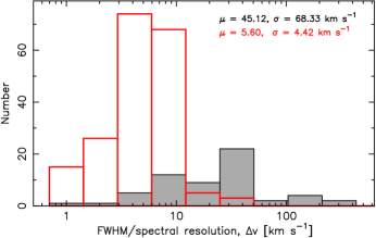
Figure 1: The distribution of spectral resolution (for the non-detections, unfilled histogram) and the line-widths (for the detections, filled histogram). The non-detections span a range of $0.29-30$ km ${\rm s}^{-1}$, which are too disparate to show clearly on a linear scale.

The detections have a mean profile width of $\left<{\rm FWHM}\right>=45$ km ${\rm s}^{-1}$, which we use to recalculate the $3\sigma$ upper limit to the integrated optical depth for each non-detection. i.e. $\int\tau_{\rm obs}dv<3(\Delta S/S_{\rm obs})\times 45$ km ${\rm s}^{-1}$ (cf. Equ. 2). Since there is no evolution in the FWHM of the intervening absorbers detected in 21-cm (Curran et al., 2016a), we do not consider any redshift dependence.

Using these and the values quoted in the literature for the detections, in Fig. 2 we show the distribution of the velocity integrated optical depth of the absorption versus the redshift.

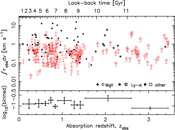
Figure 2: The velocity integrated optical depth versus the redshift for the intervening absorbers searched in H i 21-cm. The filled symbols show the detections and the unfilled circles the $3\sigma$ upper limits, with the shape representing the transition in which the absorption was initially detected: circles – Mgii, stars – Lyman-$\alpha$, squares – other (e.g. 21-cm scan). The bottom panel shows the binned values in equally sized bins (10 bins of 25), including the limits, where the horizontal error bars show the range of points in the bin and the vertical error bars the $1\sigma$ uncertainty in the mean value.

In the bottom panel, the upper limits are included in the binning as censored data points, via the Astronomy SURVival Analysis (asurv) package (Isobe et al., 1986). The points are binned via the Kaplan–Meier estimator, giving the maximum-likelihood estimate based upon the parent population (Feigelson & Nelson, 1985), from which we see no overwhelming bias in the survey sensitivity between the Mgii absorbers and DLAs.

2.2 The spin temperature/covering factor degeneracy

Since only two of the detections exhibit optically thick ($\tau_{\rm obs}>0.3$) absorption, we can, in principle, use Equ. 3 to determine the spin temperature of the gas. These two absorbers have peak optical depths of $\tau_{\rm obs}\approx 0.40$ ($z_{\rm abs}=1.3265$ towards J0850+5159) and $\tau_{\rm obs}\approx 0.55$ ($z_{\rm abs}=1.3603$ towards FBQS J2340–0053, Gupta et al. 2009b), Fig. 3,

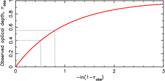
Figure 3: The variation of the observed optical depth with the intrinsic optical depth. The dotted lines show the maximum effect (where $f=1$) on the two optically thick cases.

and so the range of possible intrinsic optical depths are $\tau=0.40-0.51$ and $\tau=0.55-0.80$, respectively (since $\tau_{\rm obs}<f\leq 1$, O’Dea et al. 1994).

Since $T_{\rm spin}\propto f\,N_{\text{H{\sc\,i}}}/\int\!\tau_{\rm obs}\,dv$, we also require the covering factor to determine the spin temperature. However, without knowledge of the relative extents of the absorber–frame 1420 MHz absorption and emission cross-sections, nor the alignment between the absorber and the emitter, this is unknown. It will, however, exhibit a strong redshift dependence (Curran & Webb, 2006): In the small angle approximation, this is given by

$$f=\left\{\begin{array}[]{l l}\left(\frac{d_{\rm abs}DA_{\rm QSO}}{d_{\rm QSO}DA_{\rm abs}}\right)^{2}&\text{ if }\theta_{\rm abs}<\theta_{\rm QSO}\\ 1&\text{ if }\theta_{\rm abs}\geq\theta_{\rm QSO}\\ \end{array}\right.$$ (4)

(see Curran 2012; Allison et al. 2016b), where the angular diameter distance to a source is

$$DA=\frac{DC}{z+1},{\rm\leavevmode\nobreak\ where\leavevmode\nobreak\ }DC=\frac{c}{H_{0}}\int_{0}^{z}\frac{dz}{H_{\rm z}/H_{0}}$$ (5)

is the line-of-sight co-moving distance (e.g. Peacock 1999), in which $c$ is the speed of light, $H_{0}$ the Hubble constant and $H_{\rm z}$ the Hubble parameter at redshift $z$, given by ${H_{\rm z}}/{H_{0}}=\sqrt{\Omega_{\rm m}\,(z+1)^{3}+(1-\Omega_{\rm m}-\Omega_{\Lambda})\,(z+1)^{2}+\Omega_{\Lambda}}$. For a standard $\Lambda$ cosmology with $H_{0}=71$ km s^-1 Mpc^-1, $\Omega_{\rm matter}=0.27$ and $\Omega_{\Lambda}=0.73$, this gives a peak in the angular diameter distance at $z\approx 1.6$, which has the consequence that below this redshift $DA_{\rm DLA}\ll DA_{\rm QSO}$, as well as $DA_{\rm DLA}\sim DA_{\rm QSO}$, is possible (when $z_{\rm abs}\ll z_{\rm QSO}$), whereas above $z_{\rm abs}\sim 1.6$, only $DA_{\rm DLA}\sim DA_{\rm QSO}$ is possible. This leads a mix of angular diameter distance ratios ($DA_{\rm abs}/DA_{\rm QSO}$) at low redshift, but exclusively high values ($DA_{\rm abs}/DA_{\rm QSO}\sim 1$) at high redshift.

Although we have no information on the absorber/emitter extents nor the DLA–QSO alignment, we can at least account for this angular diameter bias, via (Equs. 3 & 4, where $\theta_{\rm abs}<\theta_{\rm QSO}$)

$$\int\!\tau_{\rm obs}\,dv\left(\frac{DA_{\rm abs}}{DA_{\rm QSO}}\right)^{2}=\frac{1}{1.823\times 10^{18}}\frac{N_{\text{H{\sc\,i}}}}{T_{\rm spin}}\left(\frac{d_{\rm abs}}{d_{\rm QSO}}\right)^{2},$$ (6)

the effect of which we show in Fig. 4.

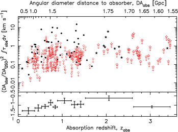
Figure 4: As Fig. 2, but corrected for the angular diameter distances (Equ. 6).

From the binned data there may be a peak in $\int\!\tau_{\rm obs}\,dv\left({DA_{\rm abs}}/{DA_{\rm QSO}}\right)^{2}$ at $z_{\rm abs}\sim 2$, which is close to where the star formation density, $\psi_{*}$, peaks ($z=2.48$, e.g. Hopkins & Beacom 2006). Since the ordinate is proportional to $(N_{\text{H{\sc\,i}}}/T_{\rm spin})\left({d_{\rm abs}}/{d_{\rm QSO}}\right)^{2}$, this could indicate a physical connection, with the abundance of cool gas peaking close to the maximum $\psi_{*}$, providing that there is no dominant evolution in ${d_{\rm abs}}/{d_{\rm QSO}}$. Without accounting for the column density, however, this only demonstrates a peak in the abundance of cold gas, rather than in its fraction.

3 Evolution of the neutral gas

3.1 Neutral gas and star formation

Although for the Mgii absorbers we do not know the individual $N_{\text{H{\sc\,i}}}$ values, from the current 21-cm emission and Lyman-$\alpha$ absorption data we do know how the mean column density, $\left<N_{\text{H{\sc\,i}}}\right>$, evolves with redshift. We can obtain this from the evolution of the cosmological mass density (Fig. 5, top) via

$$\Omega_{\text{H{\sc\,i}}}=\frac{\mu\,m_{{}_{\rm H}}\,H_{0}}{c\,\rho_{\rm crit}}\,n_{\rm DLA}\,\left<N_{\text{H{\sc\,i}}}\right>\frac{1}{(z+1)^{2}}\frac{H_{\rm z}}{H_{0}},$$ (7)

where $\mu=1.3$ is a correction for the 75% hydrogen composition, $m_{{}_{\rm H}}$ is the mass of the hydrogen atom, $\rho_{\rm crit}\equiv 3\,H_{0}^{2}/8\,\pi\,G$ is the critical mass density of the Universe, where $G$ is the gravitational constant, and $n_{\rm DLA}=0.027(z_{\rm abs}+1)^{1.682}$ (Rao et al., 2017) is the redshift number density of DLAs.

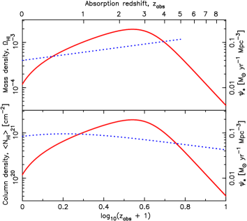
Figure 5: The best fit to the cosmological H i mass density of Crighton et al. (2017) [$\Omega_{\text{H{\sc\,i}}}=4.0\times 10^{-4}(z_{\rm abs}+1)^{0.60}$ – dotted line, top panel] and the mean column density obtained from this (bottom panel). The abscissa is mapped to $\log_{10}(z_{\rm abs}+1)$, in order to demonstrate the contrast between the evolution of $N_{\text{H{\sc\,i}}}$ and the star formation density (Hopkins & Beacom, 2006) [solid curve], where $\psi_{*}$ is arbitrarily shifted on the ordinate but retains the relative scaling (right hand scale).

We show the derived distribution of $\left<N_{\text{H{\sc\,i}}}\right>$ in Fig. 5 (bottom) and applying this to Equ. 6, we can obtain the mean evolution in $({1}/{T_{\rm spin}})\left({d_{\rm abs}}/{d_{\rm QSO}}\right)^{2}$. As per the DLAs, these appear to trace $\psi_{*}$, at least as far as the upper redshift limit of the absorbers (Fig. 6).

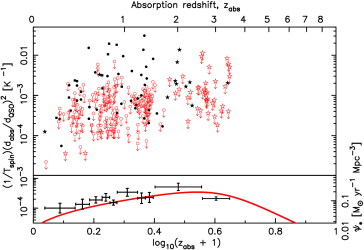
Figure 6: The reciprocal of the spin temperature degenerate with the ratio of the absorber/emitter extents (Equ. 6). As per Fig. 5, the curve shows the best fit to the SFR density (Hopkins & Beacom, 2006) arbitrarily shifted for comparison with the binned values of the top panel.

Since actual column densities are available for the confirmed DLAs, which occupy the higher redshifts (Fig. 2), in Fig. 7 we also show the distribution using the measured column densities for the DLAs, as well as applying $\left<N_{\text{H{\sc\,i}}}\right>$ to the Mgii absorbers alone.

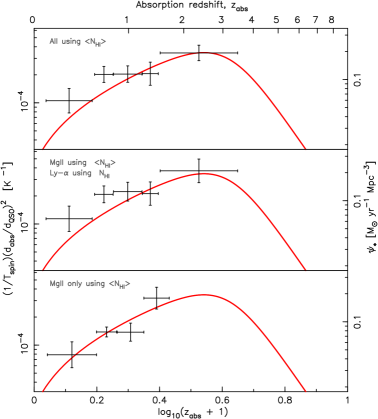
Figure 7: As Fig. 6, using the mean column density for all of the absorbers (top panel), only the Mgii absorbers normalised by $\left<N_{\text{H{\sc\,i}}}\right>$ with the DLAs normalised by the actual $N_{\text{H{\sc\,i}}}$ measurements (see Curran 2017, middle panel). In these two panels the bin size has been doubled to $n=50$ (halving the number of bins), in order to improve the signal-to-noise ratios. The bottom panel shows only the Mgii absorbers normalised by $\left<N_{\text{H{\sc\,i}}}\right>$, where the sample of 188 is binned into four bins of 47. As per Fig. 5, the curves show the SFR density arbitrarily shifted on the ordinate, where the same shift is used in each panel.

From this, we see that actual column densities are consistent with the mean values, although the uncertainties are larger because of the smaller numbers. From the bottom panel, we see that $(1/T_{\rm spin})(d_{\rm abs}/d_{\rm QSO})^{2}$ for the Mgii absorbers only also traces $\psi_{*}$, although the redshift range is more truncated (due to the $z_{\rm abs}\stackrel{{\scriptstyle<}}{{{}_{\sim}}}2.2$ limitation of ground-based Mgii spectroscopy).

In order to test the similarity between $(1/T_{\rm spin})(d_{\rm abs}/d_{\rm QSO})^{2}$ and $\psi_{*}$, in Fig. 8

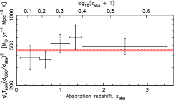
Figure 8: The SFR density normalised by $({1}/{T_{\rm spin}})\left({d_{\rm abs}}/{d_{\rm QSO}}\right)^{2}$. The hatching shows the region over which the error bars overlap, $439-457$ M_⊙ yr^-1 Mpc ^-3 K.

we show the SFR density normalised by the fraction of cool gas

$$\psi_{*}\left[\frac{1.823\times 10^{18}}{\left<N_{\text{H{\sc\,i}}}\right>}\int\!\tau_{\rm obs}\,dv\left(\frac{DA_{\rm abs}}{DA_{\rm QSO}}\right)^{2}\right]^{-1}=\psi_{*}T_{\rm spin}\left(\frac{d_{\rm QSO}}{d_{\rm abs}}\right)^{2},$$ (8)

from which the residuals are consistent with zero redshift evolution, within the $\pm 1\sigma$ uncertainties. This implies a direct correlation between these two quantities and the normalisation gives $\psi_{*}T_{\rm spin}\approx 450(d_{\rm abs}/d_{\rm QSO})^{2}$  M_⊙ yr^-1 Mpc ^-3 K, for the dependence of the star formation density upon the spin temperature (see Sect. 3.2).

3.2 Star formation and the fraction of cold neutral medium

Neutral gas in the interstellar medium is hypothesised to comprise two components (Field et al. 1969; Wolfire et al. 1995) – the cold neutral medium (CNM, where $T\sim 150$ K and $n\sim 10$ $\hbox{{\rm cm}}^{-3}$) and the warm neutral medium (WNM, where $T\sim 10\,000$ K and $n\sim 0.2$ $\hbox{{\rm cm}}^{-3}$). The CNM fraction is derived from the CNM, WNM and spin temperatures, via

$${\cal F}_{\rm CNM}\equiv{\left[{\frac{1}{T_{\rm spin}}-\frac{1}{T_{\rm WNM}}}\right]}\Bigg{/}{\left[{\frac{1}{T_{\rm CNM}}-\frac{1}{T_{\rm WNM}}}\right]},$$ (9)

giving the distribution in Fig. 9.

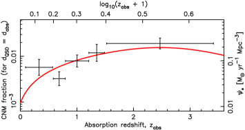
Figure 9: The redshift evolution CNM fraction and the relative star formation density.

Again, there is a reasonable trace of the star formation density, although the values are low compared to those observed, specifically ${\cal F}_{\rm CNM}\approx 0.3$ in the Milky Way (Heiles & Troland, 2003), $z_{\rm abs}=0.09$ (Lane et al., 2000) and $z_{\rm abs}=0.22$ (Kanekar et al., 2001b), getting as high as ${\cal F}_{\rm CNM}\approx 0.8$ at $z_{\rm abs}\approx 2$ (Kanekar et al., 2014). The spin temperature we derive is, however, degenerate with the ratio of the absorber/emitter extents and gives CNM fractions similar to those observed if we apply $\left<d_{\rm QSO}\right>=4\left<d_{\rm abs}\right>$ (Fig. 10).

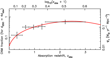
Figure 10: As per Fig. 9 but for $d_{\rm QSO}=4d_{\rm abs}$.

This ratio gives $\psi_{*}T_{\rm spin}\approx 30$ M_⊙ yr^-1 Mpc ^-3 K (cf. Fig. 8) and so for a temperature of $T_{\rm spin}\approx 300$ K, we may expect a star formation density of $\psi_{*}\approx 0.1$  M_⊙ yr^-1 Mpc ^-3. This is, of course, dependent on any evolution in $d_{\rm abs}/d_{\rm QSO}$, in addition to the assumption that the covering factor is generally less than unity (Equ. 4).

With this assumption, $d_{\rm QSO}/d_{\rm abs}$ is the only unknown in Equ. 4 and so we can use the estimate of the mean $d_{\rm QSO}/d_{\rm abs}$ ratio to determine the evolution of the mean covering factor from $DA_{\rm abs}<DA_{\rm QSO}/4$, which applies to all of sample. The mean covering factors derived are similar to those obtained from the Monte-Carlo simulation of Curran (2017) and the range of mean spin temperatures are consistent with those found in the Milky Way (Dickey et al., 2009) and other near-by galaxies (Curran et al., 2016b), $T_{\rm spin}\approx 200-2000$ K (Fig. 11).

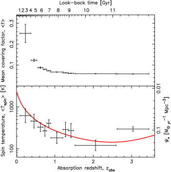
Figure 11: The estimated covering factor and spin temperature evolution, assuming $f<1$ and $d_{\rm QSO}=4d_{\rm abs}$. The curve shows $1/\psi_{*}$ (Hopkins & Beacom, 2006), scaled according to $\psi_{*}T_{\rm spin}\approx 450(d_{\rm abs}/d_{\rm QSO})^{2}$  M_⊙ yr^-1 Mpc ^-3 (Sect. 3.1).

We reiterate, however, that this assumes a mean $d_{\rm QSO}=4d_{\rm abs}$ over all redshifts and a general covering factor of less than unity.

4 Possible caveats

4.1 Column density estimates

One motivation for this work is to investigate the potential of using the evolution of the mean column density to obtain $T_{\rm spin}/f$ from the 21-cm absorption strength, where individual column density measurements will not be practical. For example, the 150 000 sight-lines to be probed in the First Large Absorption Survey in H i (FLASH) on the Australian SKA Pathfinder (ASKAP, Allison et al. 2016a). Since no UV spectrometer is planned for the James Webb Space Telescope, this will be a particular problem for the $z_{\text{H{\sc\,i}}}\stackrel{{\scriptstyle<}}{{{}_{\sim}}}1$ limitation of the SKA pathfinders (e.g. Maccagni et al. 2017) upon the demise of the Hubble Space Telescope.

From the similarities between the distributions in Fig. 7, it does appear that the estimated column densities are statistically consistent with the measured values. To test this, in Fig. 12 we show the distribution of the 21-cm line strength normalised by the mean column density, $1.823\times 10^{18}\int\!\tau_{\rm obs}\,dv/\left<N_{\text{H{\sc\,i}}}\right>=\left<f/T_{\rm spin}\right>$ (Equ. 3).

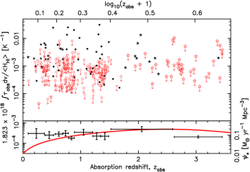
Figure 12: The estimated covering factor/spin temperature degeneracy (uncorrected for geometry), $f/T_{\rm spin}$, obtained using $\left<N_{\text{H{\sc\,i}}}\right>$.

This bears a close resemblance to the $f/T_{\rm spin}$ distribution for DLAs (Curran, 2017), where there is also a flattening of the distribution at low redshift.

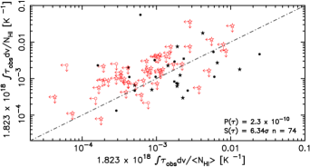
Figure 13: The actual covering factor/spin temperature degeneracy (see Curran 2017) in comparison to the estimated values (Fig. 12). The line has a gradient of unity and zero intercept. A Kendall-tau test, including the limits, gives a probability $P(\tau)=2.27\times 10^{-10}$ of the observed distribution occuring by chance, which is significant at $S(\tau)=6.34\sigma$, assuming Gaussian statistics.

In Fig. 13, we show the effect that the estimated column density has on the confirmed DLAs and sub-DLAs searched in 21-cm absorption. Although there is considerable spread, this small sample exhibits a strong correlation. This, and the similarity of Fig. 12 to the DLA distribution, gives us confidence in the application of this method to obtain a statistical estimate of the column density at a given redshift.

4.2 The correction for geometry effects

As previously stated, the above analysis assumes that there is no evolution in $d_{\rm abs}/d_{\rm QSO}$, in addition to any absorber–emitter misalignment and emitter structure being averaged out. As well as this, the covering factors are assumed to be generally less than unity. For $f<1$, $f\propto\left({DA_{\rm QSO}}/{DA_{\rm abs}}\right)^{2}$ [Equ. 4], which we see, by the comparison of Figs. 2 and 4, is the dominant effect in giving the similarity in the redshift evolution (Fig. 12 cf. 14).

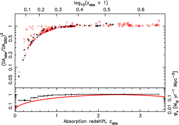
Figure 14: The evolution of the angular diameter distance ratio with redshift. Again, the solid curve in the bottom panels shows the star formation density— redshift distribution from Hopkins & Beacom (2006).

Regarding this:

1. This implies that $\psi_{*}\propto\left({DA_{\rm abs}}/{DA_{\rm QSO}}\right)^{2}$. Since the latter is purely due to geometry, there must be some more fundamental underlying parameter to which both parameters are related. This is most likely the redshift evolution which peaks at $z=2.5$, compared to $z_{\rm abs}=1.6$ for $DA_{\rm abs}/DA_{\rm QSO}$.

2. Correcting the observed optical depth by the covering factor is necessary if $f<1$ (Sect. 2.2). Although we have no information on the relative sizes nor the alignment, we do know that the geometry of the expanding Universe introduces a systematic difference in the possible values of $DA_{\rm abs}/DA_{\rm QSO}$ between the low and high redshift regimes. Thus, this must be taken into account before before making any comparison between the low and high redshift optical depths.

3. If unjustified, adding the “noise” of the 21-cm absorption strength (Fig. 12), should not improve the trace of the star formation density, otherwise this would be one coincidence on top of $DA_{\rm abs}/DA_{\rm QSO}$ exhibiting a similar evolution as $\psi_{*}$. In fact, although larger uncertainties are introduced, the product $\int\!\tau_{\rm obs}\,dv\left({DA_{\rm abs}}/{DA_{\rm QSO}}\right)^{2}$ appears to “reign in” the outliers. Specifically, the systematic offset at $z_{\rm abs}\stackrel{{\scriptstyle<}}{{{}_{\sim}}}2$ and the absence of a $z_{\rm abs}\stackrel{{\scriptstyle>}}{{{}_{\sim}}}3$ downturn (Fig. 14 cf. Fig. 6), also present in the uncorrected data (Fig. 12). Note that an increase in the spin temperature at these redshifts is also advocated by Roy et al. (2013) and Kanekar et al. (2014).

Provided that the assumptions are reasonable, the spin temperature shows a very similar evolution to the star formation density, which is diluted out by a similar evolution in the covering factor (Fig. 11), resulting in a flat distribution of $\int\!\tau_{\rm obs}\,dv\approx f\int\!\tau\,dv\propto N_{\text{H{\sc\,i}}}/T_{\rm spin}$ (Fig. 12). While further 21-cm observations of absorbers at low redshift will reduce the uncertainties introduced by $\int\!\tau_{\rm obs}\,dv$, observations at high redshift could be conclusive in determining whether $\int\!\tau_{\rm obs}\,dv\left({DA_{\rm abs}}/{DA_{\rm QSO}}\right)^{2}$ follows the downturn traced by $\psi_{*}$ (Fig. 15).

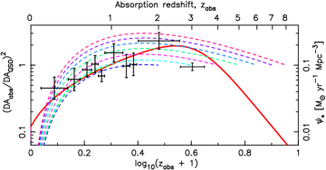
Figure 15: The star formation evolution (solid curve) and $(1/T_{\rm spin})(d_{\rm abs}/d_{\rm QSO})^{2}$ (error bars, scaled by a factor of 450, Sect. 3.2) superimposed upon the ratio of angular diameter distances for various QSO redshifts (broken curves). These are shown for $z_{\rm QSO}=1,2,...,8$ where the QSO redshift is given by the terminating value of the curve showing the absorption redshift distribution of $(DA_{\rm abs}/DA_{\rm QSO})^{2}$.

As it stands, the top bin is consistent with the ratio of angular diameter distances for $z_{\rm QSO}\approx 3-4$ and $z_{\rm abs}\stackrel{{\scriptstyle>}}{{{}_{\sim}}}2.5$, although we reiterate that a correction for the angular diameter distances is required in order to combine the low and high redshift populations. From the figure it is clear that further high redshift data, particularly at $z_{\rm abs}\stackrel{{\scriptstyle>}}{{{}_{\sim}}}4$, would be conclusive.

5 Summary

It is an outstanding problem that the total neutral gas content of intervening absorbers does not trace the star formation density, $\psi_{*}$, which shows strong evolution with redshift. Recently, however, by using the ratio of the strength of the 21-cm absorption to the total column density as a thermometer, Curran (2017) showed that the cool component of the gas could trace $\psi_{*}$. This is physically motivated, since the star formation requires that the gas be sufficiently cool for the cloud to collapse under its own gravity, this cool gas usually being evident through large molecular abundances in the “giant molecular clouds” which host the cool gas. Indeed there may be similar correlation between the ${\rm H}_{2}$ density and $\psi_{*}$, at least up to $z\sim 2$ (Lagos et al. 2014 and references therein).

The H i  data are, however, limited to a sample of 74 absorbers where both 21-cm absorption has been searched and the column density is known. By binning these in order to overcome individual line-of-sight effects, such as the absorber–QSO alignment, structure in the radio emission and situations where the covering factor may be unity, gives just three bins, which exhibit the same approximate peak at a similar relative magnitude as the star formation density (Curran, 2017). Since 21-cm absorption searches of a significantly larger sample of DLAs will most likely have to wait for the Square kilometre Array, we examine the potential of using other intervening absorption systems, where the neutral hydrogen column density is not readily available (e.g. Mg ii absorbers), to trace the star formation history. In order to do this, we:

1. Normalise the upper limits in the integrated optical depth to the same spectral resolution and include these via a survival analysis, giving a sample total of 250 absorbers.

2. Remove the bias introduced to the covering factor between the low and high redshift absorbers by the geometry effects of an expanding Universe. That is, correcting for the fact that absorbers at $z_{\rm abs}\stackrel{{\scriptstyle>}}{{{}_{\sim}}}1.6$ are always at a similar angular diameter distance as the background continuum source, whereas at lower redshift there is a mix of angular diameter distances.

3. Assign a column density derived from the evolution of the cosmological H i density.

4. Bin the data in order to average out differences in the individual line-of-sight effects.

This yields $(1/T_{\rm spin})(d_{\rm abs}/d_{\rm QSO})^{2}$, which, as for the DLAs, appears to trace the star formation density. For no evolution in the ratio of the absorber–QSO sizes, this would imply that $\psi_{*}\propto 1/T_{\rm spin}$.

As is the case for the DLA-only sample, however, data is lacking at higher redshifts ($z_{\rm abs}\stackrel{{\scriptstyle>}}{{{}_{\sim}}}3$), meaning that we cannot be certain that $(1/T_{\rm spin})(d_{\rm abs}/d_{\rm QSO})^{2}$ follows the same downturn as $\psi_{*}$ at look-back times beyond 11 Gyr. However, given that $\left<N_{\text{H{\sc\,i}}}\right>$ up to $z\sim 5$ is known, we may need only search for intervening 21-cm absorption. A non-reliance upon an optical spectrum would be advantageous to the next generation of radio band surveys, since optically selected surveys may miss the most dust reddened objects (Webster et al., 1995; Carilli et al., 1998; Curran et al., 2017). This does, however, depend upon the evolution in $\left<N_{\text{H{\sc\,i}}}\right>$ being applicable to the optically faint objects. In any case, follow-up observations of the many newly discovered 21-cm absorbers expected with the Square Kilometre Array (Morganti et al., 2015), with either 21-cm emission (limited to $z_{\rm abs}\stackrel{{\scriptstyle<}}{{{}_{\sim}}}1$, Staveley-Smith & Oosterloo 2015) or Lyman-$\alpha$ absorption (limited to $z_{\rm abs}\stackrel{{\scriptstyle>}}{{{}_{\sim}}}1.7$), will be very observationally expensive. Upon confirmation with further data, it is hoped that the methods presented here may offer a solution in determining the evolution of the cold gas fraction over large look-back times.

References

- Allison et al. (2017) Allison, J. R., Moss, V. A., Macquart, J.-P., et al. 2017, MNRAS, 465, 4450
- Allison et al. (2016a) Allison, J. R., Sadler, E. M., Moss, V. A., et al. 2016a, Astronomische Nachrichten, 337, 175
- Allison et al. (2016b) Allison, J. R., Zwaan, M. A., Duchesne, S. W., & Curran, S. J. 2016b, MNRAS, 462, 1341
- Braun (2012) Braun, R. 2012, ApJ, 87, 749
- Briggs et al. (2001) Briggs, F. H., de Bruyn, A. G., & Vermeulen, R. C. 2001, A&A, 373, 113
- Briggs & Wolfe (1983) Briggs, F. H. & Wolfe, A. M. 1983, ApJ, 268, 76
- Brown & Roberts (1973) Brown, R. L. & Roberts, M. S. 1973, ApJ, 184, L7
- Brown & Spencer (1979) Brown, R. L. & Spencer, R. E. 1979, ApJ, 230, L1
- Burgarella et al. (2013) Burgarella, D., Buat, V., Gruppioni, C., et al. 2013, A&A, 554, A70
- Carilli et al. (1998) Carilli, C. L., Menten, K. M., Reid, M. J., Rupen, M. P., & Yun, M. S. 1998, ApJ, 494, 175
- Carilli et al. (1993) Carilli, C. L., Rupen, M. P., & Yanny, B. 1993, ApJ, 412, L59
- Carilli & Walter (2013) Carilli, C. L. & Walter, F. 2013, ARA&A, 51, 105
- Chengalur et al. (1999) Chengalur, J. N., de Bruyn, A. G., & Narasimha, D. 1999, A&A, 343, L79
- Chengalur & Kanekar (2000) Chengalur, J. N. & Kanekar, N. 2000, MNRAS, 318, 303
- Crighton et al. (2015) Crighton, N. H. M., Murphy, M. T., Prochaska, J. X., et al. 2015, MNRAS, 452, 217
- Crighton et al. (2017) Crighton, N. H. M., Murphy, M. T., Prochaska, J. X., et al. 2017, in IAU Symposium, Vol. 321, Formation and Evolution of Galaxy Outskirts, ed. A. Gil de Paz, J. H. Knapen, & J. C. Lee, 309–314
- Curran (2010) Curran, S. J. 2010, MNRAS, 402, 2657
- Curran (2012) Curran, S. J. 2012, ApJ, 748, L18
- Curran (2017) Curran, S. J. 2017, MNRAS, 470, 3159
- Curran et al. (2007a) Curran, S. J., Darling, J. K., Bolatto, A. D., et al. 2007a, MNRAS, 382, L11
- Curran et al. (2016a) Curran, S. J., Duchesne, S. W., Divoli, A., & Allison, J. R. 2016a, MNRAS, 462, 4197
- Curran et al. (2004) Curran, S. J., Murphy, M. T., Pihlström, Y. M., et al. 2004, MNRAS, 352, 563
- Curran et al. (2005) Curran, S. J., Murphy, M. T., Pihlström, Y. M., Webb, J. K., & Purcell, C. R. 2005, MNRAS, 356, 1509
- Curran et al. (2016b) Curran, S. J., Reeves, S. N., Allison, J. R., & Sadler, E. M. 2016b, MNRAS, 459, 4136
- Curran et al. (2010) Curran, S. J., Tzanavaris, P., Darling, J. K., et al. 2010, MNRAS, 402, 35
- Curran et al. (2007b) Curran, S. J., Tzanavaris, P., Murphy, M. T., Webb, J. K., & Pihlström, Y. M. 2007b, MNRAS, 381, L6
- Curran et al. (2007c) Curran, S. J., Tzanavaris, P., Pihlström, Y. M., & Webb, J. K. 2007c, MNRAS, 382, 1331
- Curran & Webb (2006) Curran, S. J. & Webb, J. K. 2006, MNRAS, 371, 356
- Curran et al. (2002) Curran, S. J., Webb, J. K., Murphy, M. T., et al. 2002, PASA, 19, 455
- Curran et al. (2017) Curran, S. J., Whiting, M. T., Allison, J. R., et al. 2017, MNRAS, 467, 4514
- Curran et al. (2006) Curran, S. J., Whiting, M. T., Murphy, M. T., et al. 2006, MNRAS, 371, 431
- Darling et al. (2004) Darling, J., Giovanelli, R., Haynes, M. P., Bower, G. C., & Bolatto, A. D. 2004, ApJ, 613, L101
- Davis & May (1978) Davis, M. M. & May, L. S. 1978, ApJ, 219, 1
- Delhaize et al. (2013) Delhaize, J., Meyer, M. J., Staveley-Smith, L., & Boyle, B. J. 2013, MNRAS, 433, 1398
- Dickey et al. (2009) Dickey, J. M., Strasser, S., Gaensler, B. M., et al. 2009, ApJ, 693, 1250
- Dutta et al. (2017a) Dutta, R., Srianand, R., Gupta, N., & Joshi, R. 2017a, MNRAS, 468, 1029
- Dutta et al. (2017b) Dutta, R., Srianand, R., Gupta, N., et al. 2017b, MNRAS, 465, 4249
- Ellison et al. (2012) Ellison, S., Kanekar, N. amd Prochaska, J. X., Momjian, E., & Worseck, G. 2012, MNRAS, 424, 293
- Feigelson & Nelson (1985) Feigelson, E. D. & Nelson, P. I. 1985, ApJ, 293, 192
- Fernández et al. (2016) Fernández, X., Gim, H. B., van Gorkom, J. H., et al. 2016, ApJ, 824, L1
- Field et al. (1969) Field, G. B., Goldsmith, D. W., & Habing, H. J. 1969, ApJ, 155, L149
- Gupta et al. (2013) Gupta, N., Srianand, R., Noterdaeme, P., Petitjean, P., & Muzahid, S. 2013, A&A, 558, A84
- Gupta et al. (2012) Gupta, N., Srianand, R., Petitjean, P., et al. 2012, A&A, 544, 21
- Gupta et al. (2009a) Gupta, N., Srianand, R., Petitjean, P., Noterdaeme, P., & Saikia, D. J. 2009a, in Astronomical Society of the Pacific Conference Series, Vol. 407, The Low-Frequency Radio Universe, ed. D. J. Saikia, D. A. Green, Y. Gupta, & T. Venturi, 67
- Gupta et al. (2009b) Gupta, N., Srianand, R., Petitjean, P., Noterdaeme, P., & Saikia, D. J. 2009b, MNRAS, 398, 201
- Heiles & Troland (2003) Heiles, C. & Troland, T. H. 2003, ApJ, 586, 1067
- Hopkins & Beacom (2006) Hopkins, A. M. & Beacom, J. F. 2006, ApJ, 651, 142
- Hoppmann et al. (2015) Hoppmann, L., Staveley-Smith, L., Freudling, W., et al. 2015, MNRAS, 452, 3726
- Isobe et al. (1986) Isobe, T., Feigelson, E., & Nelson, P. 1986, ApJ, 306, 490
- Kanekar (2014) Kanekar, N. 2014, ApJ, 797, L20
- Kanekar & Briggs (2003) Kanekar, N. & Briggs, F. H. 2003, A&A, 412, L29
- Kanekar & Chengalur (2001) Kanekar, N. & Chengalur, J. N. 2001, A&A, 369, 42
- Kanekar & Chengalur (2003) Kanekar, N. & Chengalur, J. N. 2003, A&A, 399, 857
- Kanekar et al. (2001a) Kanekar, N., Chengalur, J. N., Subrahmanyan, R., & Petitjean, P. 2001a, A&A, 367, 46
- Kanekar et al. (2013) Kanekar, N., Ellison, S. L., Momjian, E., York, B. A., & Pettini, M. 2013, MNRAS, 532
- Kanekar et al. (2001b) Kanekar, N., Ghosh, T., & Chengalur, J. N. 2001b, A&A, 373, 394
- Kanekar et al. (2009) Kanekar, N., Prochaska, J. X., Ellison, S. L., & Chengalur, J. N. 2009, MNRAS, 396, 385
- Kanekar et al. (2014) Kanekar, N., Prochaska, J. X., Smette, A., et al. 2014, MNRAS, 438, 2131
- Lagos et al. (2014) Lagos, C. D. P., Baugh, C. M., Zwaan, M. A., et al. 2014, MNRAS, 440, 920
- Lah et al. (2007) Lah, P., Chengalur, J. N., Briggs, F. H., et al. 2007, MNRAS, 376, 1357
- Lane (2000) Lane, W. M. 2000, PhD thesis, University of Groningen
- Lane & Briggs (2001) Lane, W. M. & Briggs, F. H. 2001, ApJ, 561, L27
- Lane et al. (2000) Lane, W. M., Briggs, F. H., & Smette, A. 2000, ApJ, 532, 146
- Lavalley et al. (1992) Lavalley, M. P., Isobe, T., & Feigelson, E. D. 1992, in BAAS, Vol. 24, 839–840
- Lovell et al. (1996) Lovell, J. E. J., Reynolds, J. E., Jauncey, D. L., et al. 1996, ApJ, 472, L5
- Maccagni et al. (2017) Maccagni, F. M., Morganti, R., Oosterloo, T. A., Geréb, K., & Maddox, N. 2017, A&A, in press (arXiv:1705.00492)
- Madau & Dickinson (2014) Madau, P. & Dickinson, M. 2014, Ann. Rev. Astr. Ap., 52, 415
- Michałowski et al. (2015) Michałowski, M. J., Gentile, G., Hjorth, J., et al. 2015, A&A, 582, A78
- Morganti et al. (2015) Morganti, R., Sadler, E. M., & Curran, S. 2015, Advancing Astrophysics with the Square Kilometre Array (AASKA14), 134
- Neeleman et al. (2016) Neeleman, M., Prochaska, J. X., Ribaudo, J., et al. 2016, ApJ, 818, 113
- Noterdaeme et al. (2012) Noterdaeme, P., Petitjean, P., Carithers, W. C., et al. 2012, A&A, 547, L1
- O’Dea et al. (1994) O’Dea, C. P., Baum, S. A., & Gallimore, J. F. 1994, ApJ, 436, 669
- Peacock (1999) Peacock, J. A. 1999, Cosmological Physics (Cambridge: Cambridge University Press)
- Prochaska & Herbert-Fort (2004) Prochaska, J. X. & Herbert-Fort, S. 2004, PASP, 116, 622
- Prochaska et al. (2005) Prochaska, J. X., Herbert-Fort, S., & Wolfe, A. M. 2005, ApJ, 635, 123
- Prochaska & Wolfe (2009) Prochaska, J. X. & Wolfe, A. M. 2009, ApJ, 696, 1543
- Purcell & Field (1956) Purcell, E. M. & Field, G. B. 1956, ApJ, 124, 542
- Rao et al. (2006) Rao, S., Turnshek, D., & Nestor, D. B. 2006, ApJ, 636, 610
- Rao & Turnshek (2000) Rao, S. M. & Turnshek, D. A. 2000, ApJS, 130, 1
- Rao et al. (2017) Rao, S. M., Turnshek, D. A., Sardane, G. M., & Monier, E. M. 2017, MNRAS, submitted (arXiv:1704.01634)
- Rhee et al. (2013) Rhee, J., Zwaan, M. A., Briggs, F. H., et al. 2013, MNRAS, 435, 2693
- Roy et al. (2013) Roy, N., Mathur, S., Gajjar, V., & Nath Patra, N. 2013, MNRAS, 436, L94
- Sobral et al. (2013) Sobral, D., Smail, I., Best, P. N., et al. 2013, MNRAS, 428, 1128
- Spring & Michałowski (2017) Spring, E. F. & Michałowski, M. J. 2017, MNRAS, submitted (arXiv:1707.08877)
- Srianand et al. (2012) Srianand, R., Gupta, N., Petitjean, P., et al. 2012, MNRAS, 421, 651
- Staveley-Smith & Oosterloo (2015) Staveley-Smith, L. & Oosterloo, T. 2015, Advancing Astrophysics with the Square Kilometre Array (AASKA14), 167
- Webster et al. (1995) Webster, R. L., Francis, P. J., Peterson, B. A., Drinkwater, M. J., & Masci, F. J. 1995, Nat, 375, 469
- Wolfe et al. (2005) Wolfe, A. M., Gawiser, E., & Prochaska, J. X. 2005, ARA&A, 43, 861
- Wolfire et al. (1995) Wolfire, M. G., Hollenbach, D., McKee, C. F., Tielens, A. G. G. M., & Bakes, E. L. O. 1995, ApJ, 443, 152
- York et al. (2007) York, B. A., Kanekar, N., Ellison, S. L., & Pettini, M. 2007, MNRAS, 382, L53
- Zwaan et al. (2015) Zwaan, M. A., Liske, J., Péroux, C., et al. 2015, MNRAS, 453, 1268
- Zwaan et al. (2005) Zwaan, M. A., van der Hulst, J. M., Briggs, F. H., Verheijen, M. A. W., & Ryan-Weber, E. V. 2005, MNRAS, 364, 1467
- Zwart et al. (2014) Zwart, J. T. L., Jarvis, M. J., Deane, R. P., et al. 2014, MNRAS, 439, 1459