suppReferences
Non-stationary Stochastic Optimization under -Variation Measures
Abstract
We consider a non-stationary sequential stochastic optimization problem, in which the underlying cost functions change over time under a variation budget constraint. We propose an -variation functional to quantify the change, which yields less variation for dynamic function sequences whose changes are constrained to short time periods or small subsets of input domain. Under the -variation constraint, we derive both upper and matching lower regret bounds for smooth and strongly convex function sequences, which generalize previous results in Besbes et al. (2015). Furthermore, we provide an upper bound for general convex function sequences with noisy gradient feedback, which matches the optimal rate as . Our results reveal some surprising phenomena under this general variation functional, such as the curse of dimensionality of the function domain. The key technical novelties in our analysis include affinity lemmas that characterize the distance of the minimizers of two convex functions with bounded difference, and a cubic spline based construction that attains matching lower bounds.
Key words: Non-stationary stochastic optimization, bandit convex optimization, variation budget constraints, minimax regret.
1 Introduction
Non-stationary stochastic optimization studies the problem of optimizing a non-stationary sequence of convex functions on the fly, with either noisy gradient or function value feedback. This problem has important applications in operations research and machine learning, such as dynamic pricing, online recommendation services, and simulation optimization (Gur, 2014; den Boer & Zwart, 2015; den Boer, 2015; Keskin & Zeevi, 2017). For example, in the case of dynamic pricing, an analyst is given the task of pricing a specific item over a long period of time, with feedback in the form of sales volumes in each time period. As the demand changes constantly over time, the problem can be naturally formulated as non-stationary sequential stochastic optimization, where the analyst adjusts his/her pricing over time based on noisy temporal feedback data.
Formally, consider a sequence of convex functions over epochs, where is a convex, compact domain in the -dimensional Euclidean space . At each epoch , a policy selects an action , based on stochastic or noisy feedback (defined in Sec. 2) of previous epochs , and suffers loss . The objective is to compete with the dynamic optimal sequence of actions in hindsight; that is, to minimize regret
To ensure existence of policy with sub-linear regret (i.e., the non-trivial regret of ), constraints are imposed upon function sequences such that any pair of consecutive functions and are sufficiently close, and therefore feedback through previous epochs are informative for later ones. These constraints usually carry strong practical implications. For example, in dynamic pricing problems, an action represents the price and is the (negative) revenue function at time in terms of price. Since the demand functions cannot change too rapidly, it is natural to impose a constraint on adjacent pairs of revenue functions (see, e.g., Keskin & Zeevi (2017)).
The question of optimizing regret for non-stationary convex functions with stochastic feedback has received much attention in recent years. One particular interesting instance of non-stationary stochastic convex optimization was considered in Besbes et al. (2015), where sub-linear regret policies were derived when the average difference is assumed to go to zero as . Optimal upper and lower regret bounds were derived for both noisy gradient and noisy function value feedback settings.
In this work, we generalize the results of Besbes et al. (2015) so that local spatial and temporal changes of functions are taken into consideration. For any measurable function , define
| (1) |
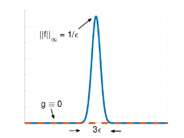
Here, is the Lebesgue measure of the domain and is finite because of the compactness of . We shall refer to as the -norm of in the rest of this paper. (Conventionally in functional analysis the norm of a function is defined as the unnormalized integration .) Nevertheless, we adopt the volume normalized definition for the convenience of presentation. It is worth noting that this normalization will not affect our results. In particular, because is a compact domain and is a constant, the regrets using the two definitions of function norm only differ by a multiplicative constant. Moreover, the Minkowski’s inequality , as well as other basic properties of norm, remains valid. Also, for a sequence of convex functions , define the -variation functional of as
| (2) |
Note that in both Eqs. (1) and (2) we restrain ourselves to convex norms and . We can then define function classes
| (3) |
which serves as the budget constraint for a function sequence . The definition of is more general than introduced in Besbes et al. (2015) since it better reflects the spatial and temporal locality of in the subscripts and .
1.1 A motivating example of dynamic pricing
To motivate the -variation constraint, we use dynamic pricing as a motivating example and illustrate the advantages of the -variation measure for loss functions with “local” spatial or temporal changes. We also provide guidelines on how values should be set qualitatively.
We consider a stylized dynamic pricing problem of a single item under changing revenue functions. Let be a collection of time periods, at each of which the item receives a pricing , . We normalize the prices so that their range is the unit interval . At time period , an unknown function characterizes the negative expected revenue a retailer collects by setting the price at . The revenue function is assumed to be non-stationary over the time periods . The objective of the retailer is to design a pricing policy such that the aggregated (negative) expected revenue is minimized.
1.1.1 Spatial (pricing) locality of revenue changes
We first fix in the variation framework and show how different values of reflect degrees of spatial (pricing) locality of the revenue functions . Suppose for all , there exists a short interval with its length such that for all , and for all . Intuitively, the assumption implies that the changes of the revenue functions between consecutive time periods are “spatially local”, and the revenues are different only at prices in a small range . This is a reasonable assumption in practice since the revenue will not be sensitive to all possible prices in (e.g., a pair of adjacent revenue function values remain the same when price is very high or very low).
Under the existing variation measure (), simple calculation shows that . On the other hand, for , the variation measure satisfies . When the “locality” level is much smaller than 1, . Furthermore, in cases where and , we have and therefore the existing algorithm/analysis in Besbes et al. (2015) cannot achieve sub-linear regret on ; on the other hand, by considering the measure, one has for all , and therefore by applying algorithm/analysis in this paper we can achieve sub-linear regret on .
1.1.2 Temporal locality of revenue changes
We next consider in the variation framework and show how different values of reflect degrees of temporal locality of the revenue function . Suppose there exists a subset if time periods , such that for all , and for all . Intuitively, this assumption implies that the revenue function has local temporal changes, meaning that the changes only in short time intervals and remains the same for most of the other times. This is a relevant assumption when demands of the item have clear temporal correlations, such as seasonal food and clothes.
Simple calculations show that, for and , the variation measure of the above described function sequence is . This demonstrates the effect of the parameter in -variation for with local temporal changes, i.e., a smaller leads to a smaller variation measure of when .
1.1.3 Guidelines on the selection of values
Though the underlying sequence of expected revenue functions is assumed to be unknown, in practice it is common that certain background knowledge or prior information is available regarding . In this section we discuss how such prior information, especially regarding the magnitude changes of and in , can qualitatively help us select the parameters in the variation measure.
We first discuss the selection of and fix the choice for the moment. Suppose we have the prior knowledge that each pairs of and differ significantly on portion of the domain by a difference of , as exemplified in Sec. 1.1.1. Then the variation of such function sequence is approximately . According to our results in Theorems 3.1–3.3, the worst-case regret is where depending on feedback types (e.g., noisy gradient or function value feedback) and (strong) convexity of . The regret can be further re-parameterized as where .
The above analysis leads to the following insights providing qualitative suggestions of choices:
-
1.
The term is smaller for smaller values, because and is a strictly decreasing function in . This suggests that for function sequences with stronger spatial locality (e.g., revenue functions that only change on a small range of prices), one should use a smaller value in -variation measure;
-
2.
The term is smaller for larger values, because and is a strictly increasing function in . This suggests that for function sequences with smaller absolute amount of perturbation, one should use a larger in -variation measure.
We next discuss the selection of and fix the choice of . Unlike the spatial locality parameter , our Theorems 3.1 and 3.2 suggest that the optimal worst-case regret is insensitive to the choice of . This might sound surprising, but is the characteristic of the adopted worst-case analytical framework. To see this, we note that the worst-case function sequence is the one that evenly distributes the function changes across all (see also the detailed construction in the online supplement), in which case the -variation measure is the same for all . It should also be noted that the choice of does not affect our optimization algorithm or its re-starting procedure. Therefore, we simply recommend the selection of but we choose to include in our theorem statements for mathematical generality.
1.2 Results and techniques
The main result of this paper is to characterize the optimal regret over function classes , which includes explicit algorithms that are computationally efficient and attain the regret, and a lower bound argument based on Fano’s inequality (Ibragimov & Has’minskii, 1981; Yu, 1997; Cover & Thomas, 2006; Tsybakov, 2009) that shows the regret attained is optimal and cannot be further improved. Below is an informal statement of our main result (a formal description is given in Theorems 3.1 and 3.2):
Main result (informal).
For smooth and strongly convex function sequences under certain regularity conditions, the optimal regret over is with noisy gradient feedback, and with noisy function value feedback, provided that is not too small. In addition, for general convex function sequences satisfying only Lipschitz continuity on function values, we obtain a regret upper bound of with noisy gradient feedback, provided that is not too small. Here is the dimension of the domain .
We clarify that our results also cover the case of small , i.e., converges to 0 as at a very fast rate. However, the case of “not too small ” is of more interest. This is because if is very small, meaning that the underlying function sequence is close to a stationary one (i.e., ), then one could re-produce the standard and/or regrets ( for strongly convex and smooth functions with noisy function feedback, for strongly convex and smooth functions with noisy gradient feedback, and for general convex functions with noisy gradient feedback; see also, e.g., Jamieson et al. (2012); Agarwal et al. (2010); Hazan et al. (2007).) These rates are also known to be optimal (Jamieson et al., 2012; Hazan & Kale, 2014). Technical details of this point are given in the statements of Theorems 3.1, 3.2, 3.3.
More importantly, our result reveals several interesting facts about the regret over function sequences with local spatial and temporal changes. Most surprisingly, the optimal regret suffers from curse of dimensionality, as the regret depends exponentially on the domain dimension . Such phenomenon does not occur in previous works on stationary and non-stationary stochastic optimization problems. For example, for the case of being strongly convex and smooth, as spatial locality in becomes less significant (i.e., ), the optimal regrets approach (for noisy gradient feedback) and (for noisy function value feedback), which recovers the dimension-independent regret bounds in Besbes et al. (2015) derived for the special case of and . Similar phenomenon of curse of dimensionality also appears in the general convex case. We also note that, when is not too small, the obtained regret bound matches the optimal rate for in Besbes et al. (2015) as .
To obtain results for general -variation and the optimal regrets for strongly convex case, we make several important technical contributions in this paper, which are highlighted as follows.
-
1.
For noisy function value feedback, instead of using the online gradient descent (OGD) from Besbes et al. (2015), we adopt a regularized ellipsoidal (RE) algorithm from Hazan & Levy (2014) and extend it from exact function value evaluation to the noisy version. Our analysis relaxes an important assumption in Besbes et al. (2015) that requires the optimal solution to lie far away from the boundary of . Our policy based on the RE algorithm allows the optimal solution to be closer to the boundary of as increases.
-
2.
On the upper bound side, we prove an interesting affinity result (Lemma 4.2) which shows that the optimal solutions of cannot be too far apart provided that both are smooth and strongly convex functions, and is upper bounded. The affinity result is also generalizable to non-strongly convex functions (Lemma C.2), by directly integrating function differences in a close neighborhood of (or ) without resorting to (that could be unbounded without strong convexity). Both affinity results are key in deriving upper bounds for our problem, and have not been discovered in previous literatures. They might also be potentially useful for other non-stationary stochastic optimization problems (e.g., adaptivity to unknown parameters (Besbes et al., 2015; Karnin & Anava, 2016)).
-
3.
On the lower bound side, we present a systematic framework to prove lower bounds by first reducing the non-stationary stochastic optimization problem to an estimation problem with active queries, and then applying the Fano’s inequality with a “sup-argument” similar in spirit to Castro & Nowak (2008) that handles the active querying component. To adapt Fano’s inequality, we also design a new construction of adversarial function sets, which is quite different from the one in Besbes et al. (2015). More specifically, to prove that the regret exhibits “curse of dimensionality”, one needs to construct functions that not only have different minima but also “localized” difference (meaning that for most ) such that is small. To construct such adversarial functions, we use the idea of “smoothing splines” from nonparametric statistics that connects two pieces of quadratic functions using a cubic function to ensure the smoothness and strong convexity of the constructed functions. Our analytical framework and spline-based lower bound construction could inspire new lower bounds for other online and non-stationary optimization problems.
1.3 Related work
In addition to the literature discussed in the introduction, we briefly review a few additional recent works from machine learning and optimization communities.
Stationary stochastic optimization.
The stationary stochastic optimization problem considers a stationary function sequence , and aims at finding a near-optimal solution such that is close to . When only noisy function evaluations are available at each epoch, the problem is also known as zeroth-order optimization and has received much attention in the optimization and machine learning community. Classical approaches include confidence-band methods (Agarwal et al., 2013) and pairwise comparison based methods (Jamieson et al., 2012), both of which achieve regret with polynomial dependency on domain dimension . Here in notation we drop poly-logarithmic dependency on . The tight dependency on , however, remains open. In the more restrictive statistical optimization setting , optimal dependency on can be attained by the so-called “two-point query” model (Shamir, 2015).
Online convex optimization.
In online convex optimization, an arbitrary convex function sequence is allowed, and the regret of a policy is compared against the optimal stationary benchmark in hindsight. Unlike the stochastic optimization setting, in online convex optimization the full information of is revealed to the optimizing algorithm after epoch , which allows for exact gradient methods. It is known that for unconstrained online convex optimization, the simplest gradient descent method attains regret for convex functions, and regret for strongly convex and smooth functions, both of which are optimal in the worst-case sense (Hazan, 2016). For constrained optimization problems, projection-free methods exist following mirror descent or follow-the-regularized-leader (FTRL) methods (Hazan & Levy, 2014). Zinkevich (2003); Hall & Willett (2015) considered the question of online convex optimization by competing against the optimal dynamic solution sequence subject to certain smoothness constraints like . Jadbabaie et al. (2015); Mokhtari et al. (2016) further imposed the constraint on both solution sequences and function sequences in terms of -variation and showed that adaptivity to the unknown smoothness parameter is possible with noiseless gradient and the information of . Daniely et al. (2015); Zhang et al. (2017) also designed algorithms that adapt to the unknown smoothness parameter, under the model that the entire function is revealed after time . However, the adaptation still remains an open problem in the “bandit” feedback setting considered in our paper, in which only noisy evaluations of or are revealed. Under the bandit feedback setting, the function perturbations (e.g., ) cannot be easily estimated, making it unclear whether adaptation to is possible.
Bandit convex optimization.
Bandit convex optimization is a combination of stochastic optimization and online convex optimization, where the stationary benchmark in hindsight of a sequence of arbitrary convex functions is used to evaluate regrets. At each time , only the function evaluation at the queried point (or its noisy version) is revealed to the learning algorithm. Despite its similarity to stochastic and/or online convex optimization, convex bandits are considerably harder due to its lack of first-order information and the arbitrary change of functions. Flaxman et al. (2005) proposed a novel finite-difference gradient estimator, which was adapted by Hazan & Levy (2014) to an ellipsoidal gradient estimator that achieves regret for constrained smooth and strongly convex bandits problems. For the non-smooth and non-strongly convex bandits problem, the recent work of Bubeck et al. (2017) attains regret with an explicit algorithm whose regret and running time both depend polynomially on dimension .
1.4 Notations and basic properties of
For a -dimensional vector we write to denote the norm of , for , and to denote the norm of . Define and as the -dimensional ball and sphere of radius , respectively. We also abbreviate and . For a -dimensional subset , denote as the interior of , as the closure of , and as the boundary of . For any , we also define as the “strict interior” of , where every point in is guaranteed to be at least away from the boundary of .
We note that the defined in (2) is monotonic in and , as shown below:
Proposition 1.1.
For any and it holds that . In addition, for any we have , and similarly for any we have , assuming all functions in are continuous.
The rest of the paper is organized as follows. In Section 2, we introduce the problem formulation. Section 3 contains the main results and describes the policies. Section 4 presents the proof of our main positive result. The concluding remarks and future works are discussed in Section 6. Additional proofs can be found in the online supplement.
2 Problem formulation
Suppose are a sequence of unknown convex differentiable functions supported on a bounded convex set . At epoch , a policy selects a point (i.e., makes an action) and suffers loss . Certain feedback is then observed which can guide the decision of actions in future epochs. Two types of feedback structures are considered in this work:
-
-
Noisy gradient feedback: , where is the gradient of evaluated at , and are independent -dimensional random vectors such that each component is a random variable with ; furthermore, conditioned on is a sub-Gaussian random variable with parameter , meaning that for all ;
-
-
Noisy function value feedback: , where are independent univariate random variables that satisfy ; furthermore, conditioned on is a sub-Gaussian random variable with parameter , meaning that for all .
Both feedback structures are popular in the optimization literature and were considered in previous work on online convex optimization and stochastic bandits (e.g., Hazan (2016) and references therein). For notational convenience, we shall use or simply to refer to a general feedback structure without specifying its type, which can be either or .
Apart from being closed convex and being convex and differentiable, we also make the following additional assumptions on the domain and functions :
-
(A1)
(Bounded domain): there exists constant such that ;
-
(A2)
(Bounded function and gradient): there exists constant such that and ;
-
(A3)
(Unique interior optimizer): there exists unique such that . Furthermore, the interior of is a non-empty set (i.e., ) and there exists such that .
-
(A4)
(Smoothness): there exists constant such that for all .
-
(A5)
(Strong convexity): there exists constant such that for all .
The assumptions (A1), (A2) are standard assumptions that were imposed in previous works on both stationary and non-stationary stochastic optimization (Flaxman et al., 2005; Agarwal et al., 2013; Shamir, 2015; Besbes et al., 2015). The condition (A3) assumes that the optimal solution is not too close to the boundary of the domain . Compared to similar assumptions in existing work (Flaxman et al., 2005; Besbes et al., 2015), our assumption is considerably weaker since can be within distance to the boundary; while in Flaxman et al. (2005); Besbes et al. (2015), must be distance away from the boundary (i.e., away from the boundary by at least a constant). Finally, the conditions (A4) and (A5) concern second-order properties of and enable smaller regret rates for gradient descent algorithms. We note that the condition in Besbes et al. (2015) (see Eq. (10) in Besbes et al. (2015)) is stronger and implies our (A4) and (A5) since we do not assume that is twice differentiable. We also consider parameters in (A1)–(A5) and domain dimensionality as constants throughout the paper and omit their (polynomial) multiplicative dependency in regret bounds. In Section 3.2, we further relax the assumptions (A3)–(A5) and provide upper bound results for general convex function sequences.
Let be a random quantity defined over a probability space. A policy that outputs a sequence of is admissible if it is a measurable function that can be written in the following form:
Let denote the class of all admissible policies for epochs. A widely used metric for evaluating the performance of an admissible policy is the regret against dynamic oracle :
| (4) |
Here is either the noisy gradient feedback or the noisy function feedback . Note that a unique minimizer exists due to the strong convexity of (condition A5). The goal of this paper is to characterize the optimal regret:
| (5) |
and find policies that achieve the rate-optimal regret, i.e., attain the optimal regret up to a polynomial of factor. The optimal regret in (5) is also known as the minimax regret in the literature, because it minimizes over all admissible policies and maximizes over all convex function sequences .
3 Main results
We establish theorems giving both upper and lower bounds on worst-case regret for both noisy gradient feedback and noisy function feedback over . The policies for achieving the following upper bound result will be introduced in the next section.
Theorem 3.1 (Upper bound for strongly-convex function sequences).
Fix arbitrary and . Suppose (A1) through (A5) hold, and . Then there exists a computationally efficient policy and for some function that is a polynomial function in and , such that
For the noisy function value feedback, there exists another computationally efficient policy and for some function that is a polynomial function in and , such that
Theorem 3.2 (Minimax lower bound for strongly-convex function sequences).
Suppose the same conditions hold as in Theorem 3.1. Then there exists a constant independent of and such that
In Theorem 3.1, the quantities and depend on and only via poly-logarithmic factors and these poly-log factors are usually not the focus of studying the regret. In Theorem 3.2 the quantity is independent of and . The other problem dependent parameters are treated as constants throughout the paper. The proof of Theorem 3.1 is given in Sec. 4, while the proofs of Theorem 3.2 is relegated to the online supplement.
The condition in both Theorems 3.1 and 3.2 is necessary for obtaining a non-trivial sub-linear regret. In particular, the lower bound results in Theorem 3.2 show that for , no algorithm can achieve sub-linear regret in either feedback models. On the other hand, a trivial algorithm that outputs for an arbitrary leads to a linear regret.
Both upper and lower regret bounds in Theorems 3.1 and 3.2 consist of two terms. The term for and term for arise from regret bounds for stationary stochastic optimization problems (i.e., ), which were proved in Jamieson et al. (2012); Hazan & Kale (2014). The other terms involving polynomial dependency on are the main regret terms for typical dynamic function sequences whose perturbation is not too small.
We also remark that the parameter does not affect the optimal rate of convergence in Theorem 3.2 (provided that is assumed for convexity of the norms). While this appears counter-intuitive, this is a property of our worst-case analytical framework, as the function sequence that leads to the worst-case regret is the one that distributes function changes evenly across all (see for example our detailed construction of adversarial function sequences in the online supplement), in which case the -variation measure is the same for all .
Remark 3.1 (Comparing with Besbes et al. (2015)).
Besbes et al. (2015) considered the special case of and , and established the following result:
| (6) |
Note that in Eq. (6) we adopt a slightly different notation from Besbes et al. (2015). In particular, the parameter in our paper is times the parameter in (Besbes et al., 2015). Such normalization is for presentation clarity only (to single out the term in the regret bounds).
Remark 3.2 (Curse of dimensionality).
A significant difference between and settings is the curse of dimensionality. In particular, when the (optimal) regret depends exponentially on dimension , while for the dependency on is independent of on the exponent. The curse of dimensionality is a well-known phenomenon in non-parametric statistical estimation (Tsybakov, 2009).
Below we first introduce the policies, which is based on a “meta-policy” in Besbes et al. (2015).
3.1 Policies
We first describe a “meta-policy” proposed in Besbes et al. (2015) based on a re-starting procedure:
Meta-policy (restarting procedure): input parameters and ; sub-policy . 1. Divide epochs into batches such that , , etc., with , and for . The epochs are divided as evenly as possible, so that for all . 2. For each batch , , do the following: (a) Run sub-policy with and , corresponding to .
The key idea behind the meta-policy is to “restart” certain sub-policy after epochs. This strategy ensures that the sub-policy has sufficient number of epochs to exploit feedback information, while at the same time avoids usage of outdated feedback information. For the noisy gradient feedback , we set if and otherwise; for the noisy function value feedback , we set if and otherwise. Motivations of our scalings are given in Sec. 4 in which we prove Theorem 3.1.
The sub-policy is carefully designed to exploit information provided from different types of feedback structures. For noisy gradient feedback , a simple online gradient descent (OGD, see, e.g., Besbes et al. (2015); Hazan (2016)) policy is used:
Sub-policy (OGD): input parameters ; step sizes . 1. Select arbitrary . 2. For to do the following: (a) Suffer loss and obtain feedback . (b) Compute , where .
For noisy function value feedback , the classical approach is to first obtain an estimator of the gradient by perturbing along a random coordinate . This idea originates from the seminal work of Yudin & Nemirovskii (1983) and was applied to convex bandits problems (e.g., Flaxman et al. (2005); Besbes et al. (2015)). Such an approach, however, fails to deliver the optimal rate of regret when the optimal solution lies particularly close to the boundary of the domain . Here we describe a regularized ellipsoidal (RE) algorithm from Hazan & Levy (2014), which attains the optimal rate of regret even when is very close to .
The RE algorithm in Hazan & Levy (2014) is based on the idea of self-concordant barriers:
Definition 3.1 (self-concordant barrier).
Suppose is convex and . A convex function is a -self-concordant barrier of if it is three times continuously differentiable on and has the following properties:
-
1.
For any , if then .
-
2.
For any and it holds that and where .
It is well-known that for any convex set with non-empty interior , there exists a -self-concordant barrier function with , and furthermore for bounded the barrier can be selected such that it is strictly convex; i.e., for all (Nesterov & Nemirovskii, 1994; Boyd & Vandenberghe, 2004). For example, for linear constraints with , a logarithmic barrier function can be used to satisfy all the above properties (note that denotes the -th row of ).
We are now ready to describe the RE sub-policy that handles noisy function value feedback. The policy is similar to the algorithm proposed in Hazan & Levy (2014), except that noisy function value feedback is allowed in our policy, while Hazan & Levy (2014) considered only exact function evaluations. The analysis of our policy is also more involved for dealing with noise.
Sub-policy (RE): input parameters ; constant step size ; self-concordant barrier ; 1. Select ; 2. For to do the following: (a) Compute , where is the identity matrix in . (b) Sample from the uniform distribution on the unit -dimensional sphere . (c) Select ; suffer loss and obtain feedback . (d) Compute gradient estimate . (e) FTRL update: .
In step 2(d), the gradient estimate satisfies by the change-of-variable formula and the smoothness of . In step 2(e), instead of the projected gradient step, a Follow-The-Regularized-Leader (FTRL) step is executed to prevent from being too close to the boundary of . The FTRL step is essentially a mirror descent, which uses a regularization term ( in our policy) and its associated Bregman divergence to improve the convergence rates of optimization algorithms measured in non-standard metric. It was shown in McMahan (2017) (Sec. 6) that the FTRL step is equivalent to mirror descent under minimal regularity conditions. Finally, step 2(c) is a random perturbation step originally considered in (Hazan & Levy, 2014). An important aspect of step 2(c) is the clever choice of the matrix , which ensures the optimal regret bound even if the optimal solution is very close to the boundary of . More specifically, the following proposition shows that always belongs to the domain , justifying the correctness of policy . Its proof is given in the online supplement.
Proposition 3.1.
Suppose is strictly convex on . Then for any , and ,
3.2 Extension to general convex function sequences
In this section we show that for the noisy gradient feedback case , our upper bound can be extended to general convex functions that do not necessarily satisfy smoothness (A4) or strong convexity (A5). The assumption (A3) that requires unique interior minimizer can also be removed. Our result is summarized in the following theorem:
Theorem 3.3 (Upper bound for general convex function sequences).
Fix arbitrary and . Suppose (A1) through (A2) hold, and . Also suppose that the meta-policy is carried out with the OGD sub-policy and step sizes . Then there exists for some function that is also a polynomial function in and , such that
We remark that as , the regret upper bound derived in Theorem 3.3 approaches , which matches the result in Besbes et al. (2015) for the case. Since is proved to be optimal for the case in Besbes et al. (2015), this implies the optimality of our Theorem 3.3 for the case as well. However, for , it is still an open question on establishing a tight minimax lower bound.
The structure of the proof of Theorem 3.3 is similar to the one for Theorem 3.1. It is important to note that since strong convexity is no longer assumed, the important “affinity lemma” cannot be proved by analyzing . Instead, we prove another version of “affinity lemma” (see Lemma C.2 in Sec. C) by developing new strategies that directly bound perturbation of function values. The proof of Theorem 3.3 is provided in Sec. C in the supplement.
Also note that for the general convex setting with noisy function value feedback, even the case of remains a challenging open problem (see Besbes et al. (2015)); which is left as future work.
4 Proof of Theorem 3.1
In this section we provide the complete proof of our main positive result (upper bound) in Theorem 3.1 for strongly smooth and convex function sequences . Due to space constraints, the proofs of Theorems 3.2 and 3.3 as well as Lemma 4.1 are presented in the online supplement.
Our proof of Theorem 3.1 is roughly divided into three steps. In the first step, we review existing results for the OGD and the RE algorithms on upper bounding the weak regret against stationary benchmarks. In the second step, we present a novel local integration analysis that upper bounds the gap between regret against stationary and dynamic benchmarks using the -norm difference between two smooth and strongly convex functions. Finally, we use a sequence of Hölder’s inequality to analyze the restarting procedure in the meta-policy described in the previous section.
4.1 Regret against stationary benchmarks.
For a sequence of convex functions , an admissible policy and a feedback structure , the weak regret against any stationary point is defined as
| (7) |
Compared to the regret against dynamic solution sequence defined in Eq. (5), in the benchmark solution is forced to be stationary among all epochs, resulting in smaller regret. In fact, it always holds that for any and . In the remainder of this section, we shall refer to as the “weak regret” and as the “strong regret”.
The next lemma states existing results on upper bounding the weak regret of both OGD and RE policies for adversarial function sequences . The result for OGD is folklore and documented in Hazan (2016); Besbes et al. (2015). For the RE algorithm, we extend the weak regret bound in Hazan & Levy (2014) from the exact function value feedbacks to noisy feedbacks and establish the following lemma. The proof of Lemma 4.1 is deferred to Section A in the online supplement.
Lemma 4.1.
Fix . Let be an arbitrary sequence of smooth and strongly convex functions satisfying (A1) through (A5). For noisy gradient feedback and the OGD policy, the following holds with :
| (8) |
In addition, for noisy function value feedback and the RE policy, suppose is a strictly convex -self-concordant barrier of , with , and . Then
| (9) |
Recall the definition that is the strict interior of that is at least apart from . Also, in both results we omit dependency on and .
4.2 Gap between weak and strong regret.
By definition, the gap between and is independent of policy :
| (10) |
Eq. (10) shows that it is possible to upper bound the regret gap by the two-point difference of each function evaluated at the optimal solution of and the optimal solution of , for arbitrary . Such differences, however, can be large as could be far away from as the functions drift. In the special case of , Besbes et al. (2015) observes
| (11) |
and further bounds both and with . Such arguments, however, meet significant challenges in the more general setting when , because the difference between two functions at one point can be arbitrarily larger than the -norm of the difference of the two functions. We give an illustrative example in Figure 1, where two functions and are presented, with for and .
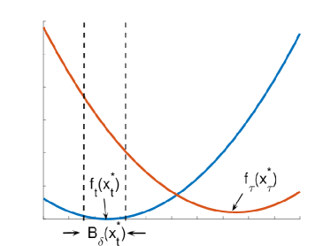
In this paper we give an alternative analysis that directly upper bounds the left-hand side of Eq. (11), (i.e., the difference of the same function at two points) using , The following is our key affinity lemma:
Lemma 4.2.
Suppose . Fix , and let be the minimizers of and , respectively. Then under (A1) through (A5) we have that
Proof.
Proof of Lemma 4.2. Without loss of generality we assume throughout this proof. Define . We first prove that , where .
Assume by way of contradiction that . For any and define . It is easy to verify that and (recall that is the diameter of ). In addition, , because , where is the deflation of by a specific vector, and similarly . Now set , and note that because . By strong convexity of , we have ,
| (12) | ||||
| (13) |
Here Eq. (12) holds because , and Eq. (13) is true because and for all . On the other hand, by smoothness of , we have that
| (14) |
Combining Eqs. (13,14) we have that, for arbitrary and
| (15) |
provided that , which holds true because by definition. Integrating both sides of Eq. (15) on and recalling the definition of , we have that
where the last equality holds because and . With , we have that and hence the contradiction.
We have now established that . By smoothness of and ,
The proof of Lemma 4.2 is then completed by plugging in . ∎
4.3 Analysis of the re-starting procedure.
We focus on the noisy gradient feedback first and briefly remark at the end of this section on how to handle noisy function value feedback. Recall that the epochs are divided into batches in the meta-policy, with each batch having either or epochs. Applying Lemmas 4.1, 4.2 together with Eq. (10) we have
| (16) |
Here the last inequality holds because (assuming without loss of generality that ) .
We next present another key lemma that upper bounds the critical summation term in Eq. (16) using , and . The proof is based on consecutively applying the Hölder’s inequality.
Lemma 4.3.
Suppose , and . Then
Proof.
4.4 Completing the proof
We now prove Theorem 3.1 by combining Lemmas 4.1, 4.2 and 4.3 with Eq. (16) and setting appropriately. First consider the noisy gradient feedback case . By Eq. (16),
Subsequently invoking Lemma 4.3 we have
where . If , then we set , and obtain regret . Otherwise, when , one selects and notes that . This yields a regret of , where in we drop poly-logarithmic dependency on .
Finally we describe how the above analysis can be generalized to the noisy function value feedback case . By Lemma 4.1, for . Subsequently,
If , then we set , and obtain regret . Otherwise, when , one selects and observes that . This yields a regret of .
5 Numerical results


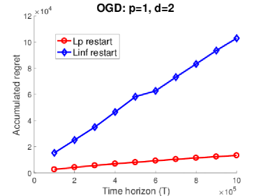
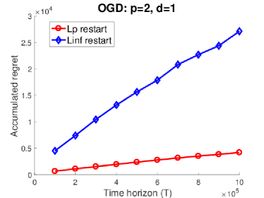
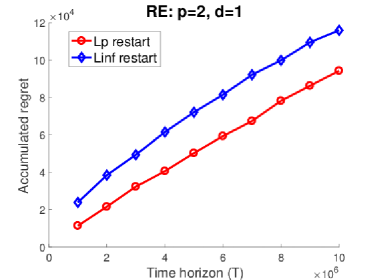
We compare our restarting procedure under -variation measure with the algorithm in Besbes et al. (2015). We choose , , and let take values in to demonstrate performance in terms of the accumulated regret. The underlying function sequence is constructed using the adversarial construction in Sec. B which is also used to prove our lower regret bound (see Theorem 3.2). In particular, we use the function constructions in Eqs. (32,35,37) and its multi-variate extension in Eq. (38) in the online supplement.
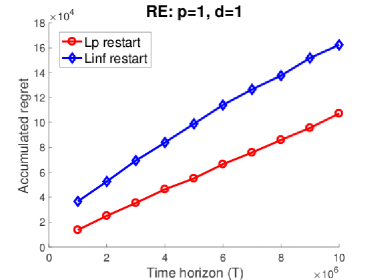
In our simulations, both the OGD and the RE algorithm (after each restarting point) are initialized at , making it at the center of the domain . For OGD, the step size is set as ; for the RE algorithm, we use the log-barrier function with step size rules , where is the number of iterations between two restarting points. For the restarting OGD/RE algorithm with -variation (red lines in Figure 2), the restarting points are selected using and directly (more specifically, or ). For the restarting OGD/RE algorithm in Besbes et al. (2015), we first utilize the knowledge of the underlying function sequence to calculate the -variation measure , and then set the restarting points using the rules or according to Besbes et al. (2015).
Figure 2 plots the accumulated regret of our compared algorithms for different underlying function sequences. For the OGD algorithms with noisy gradient feedback, the time horizon () ranges from to ; for the RE algorithms, we took to range from to since convergence is slower with only noisy function value feedback. Each algorithm is given 20 independent runs and the median accumulated regret is reported. It is observed that our algorithm (the red lines) always achieve smaller regret and outperform its competitor for constructed function sequences.
6 Concluding remarks and open questions
We considered optimal regret of non-stationary stochastic optimization with local spatial and temporal changes. An important open question is to study the optimal regret for the case of general convex functions. In Theorem 3.3 we proved an upper regret bound of for general convex function sequences with access to noisy gradient oracles, which matches the tight rate of in (Besbes et al., 2015) as . However, for , it is not clear whether our bound is tight even for the univariate case of . To further improve the learning algorithm with sharper upper bounds or to develop matching lower bound will be a future direction of research.
Acknowledgement
The authors are very grateful to three anonymous referees, the associate editor, and the area editor for their detailed and constructive comments that considerably improved the quality of this paper. We would also like to thank Prof. Assaf Zeevi for helpful discussions.
Appendix A Proof of Lemma 4.1
To simplify notations we assume throughout this proof. We first consider the noisy gradient feedback case . Fix arbitrary and abbreviate , . By strong convexity of , we have that
| (20) |
On the other hand, because by definition and is a contraction, we have
Using Pythagorean’s theorem and the fact that , and , we have
Subsequently,
| (21) |
Combining Eqs. (20,21) and summing over , and defining , we have
Because is arbitrary, we conclude that for , and all .
We next consider the noisy function value feedback case . Abbreviate and define, for any invertible matrix , that
where is uniformly distributed on the -dimensional unit ball . It is easy to verify that remains strongly convex with parameter and is an unbiased estimator of :
Here in (a) we invoke Corollary 6 of (Hazan & Levy, 2014).
Recall the definition that , the point in at which loss is suffered and feedback is obtained. For any , decompose the regret as
| (22) |
The first three terms on the right-hand side of Eq. (22) are easy to bound. In particular, because almost surely, we have that
Here in (b) we use the fact that is smooth (A4) with parameter . Similarly,
In addition, because is convex, by Jensen’s inequality we have for all and hence
We next upper bound the final term in the right-hand side of Eq. (22). For and define . Also define . It is obvious that is strongly convex with parameter , and that agrees with the definition of in step 2(e) of sub-policy , because both and terms are independent of to be optimized. We then have the following lemma, which is similar to Lemma 11 in (Hazan & Levy, 2014).
Lemma A.1.
Suppose for all . Then
| (23) |
The verification of the condition and an proof of Lemma 23 is technical and will be presented later in this section. Taking expectations on both sides of Eq. (23) and noting that and , we have
Here (c) holds because and in (d) we invoke Lemma 23.
On the other hand, because is strongly convex with parameter , it holds that and hence
Subsequently,
It then remains to upper bound the expectation of and the discrepancy of self-concordant barrier functions . By assumption (A2), we have that . Therefore,
To bound the discrepency in self-concordance barrier terms, we cite Lemma 4 from (Hazan & Levy, 2014), which asserts that for all ,
where is the self-concordance parameter of and is defined as . It is easy to verify that, for all and , because . Consequently, by Assumption (A2) and the fact that (because ) we have that
Combining all upper bounds on the terms in Eq. (22) we obtain
With we complete the proof of Lemma 4.1.
A.1 Verification of condition
We have that . By standard concentration results for sub-Gaussian random variables, we know that with probability at least . Let denote the event that . By the law of total expectation,
Here the second inequality holds because and due to assumption (A3). This term can then be upper bounded by and essentially neglected in the final regret bound. For the main term conditioned on , we have for all . Therefore, by setting we have that conditioned on .
A.2 Proof of Lemma 23
By definition of , we have that . By standard analysis of mirror descent we have that
It remains to upper bound . For define and recall that . By definition, and are dual norms and hence by Hölder’s inequality
| (24) |
Denote , where is a constant that does not depend on and . Recall the definition of
in classical self-concordance analysis. It is easy to verify that and , because . The following lemma is standard in analysis of Newton’s method for self-concordant functions:
Lemma A.2.
Suppose is -self-concordant and . Then
Note that because is self-concordant, is also self-concordant and . In addition, because is the minimizer of , 111 is defined as . and therefore
Therefore . Invoking Lemma A.2 we have that, under the condition that ,
| (25) |
Combining Eqs. (24,25) we have that . The proof is of Lemma 23 is then complete.
Appendix B Proof of Theorem 3.2
Let us first consider the simpler univariate case (). The first step is to reduce the problem of lower bounding regret to the problem of lower bounding success probability of testing sequences of functions, for which tools from information theory such as Fano’s lemma (Ibragimov & Has’minskii, 1981; Yu, 1997; Cover & Thomas, 2006; Tsybakov, 2009) could be applied. We then present a novel construction of two functions satisfying (A1) through (A5) and demonstrate that such construction leads to matching lower bounds as presented in Theorem 3.2. Finally, we extend the lower bound construction to multiple dimensions () via a change-of-variable argument and complete the proof of general cases in Theorem 3.2.
Before introducing the proof we first give the definition of an important concept that measures the “discrepancy” between two functions :
Intuitively, characterizes the best regret one could achieve without knowing whether or is the underlying function. This quantity plays a central role in our reduction from regret minimization to testing problems, as well as construction of indistinguishable functions pairs.
B.1 From regret minimization to testing.
Consider a finite subset . The following lemma shows that if there exists an admissible policy that achieves small regret over , then it leads to a hypothesis testing procedure that identifies the true function sequence in with large probability:
Lemma B.1.
Fix , and . Let or be either the noisy function or noisy gradient feedback. Let be a finite subset of sequences of convex functions. Suppose there exists an admissible policy such that
| (26) |
then there exists an estimator such that
| (27) |
where denotes the probability distribution parameterized by the underlying true function sequence .
The proof of Lemma B.1 is technical and given later. At a higher level, when there exists an admissible policy that achieves small regret over (and hence small regret over too), then one can correctly identify the underlying function sequence with large probability by searching all function sequences in and selecting the one that has the smallest regret.
Reduction to testing is a standard approach for proving minimax lower bounds in stochastic estimation and optimization problems (Besbes et al., 2015; Agarwal et al., 2012; Raskutti et al., 2011). Motivations behind such reduction are a well-established class of tools that provide lower bounds on failure probability in testing problems (Yu, 1997; Ibragimov & Has’minskii, 1981; Tsybakov, 2009). Let denote the Kullback-Leibler divergence between two distributions and . We introduce the following version of the Fano’s inequality,
Lemma B.2 (Fano’s inequality).
Let be a finite parameter set of size . For each , let be the distribution of observations parameterized by . Suppose there exists such that for all . Then
| (28) |
With Lemmas B.1 and 28, the question of proving Theorem 3.2 is reduced to finding a “hard” subset such that the minimum discrepancy is lower bounded and the maximum KL divergence is upper bounded. More precisely, the upper bound on the maximum KL divergence will provide a lower bound for right hand side of Eq. (28), which contradicts Eq. (27) in Lemma B.1. Therefore, the inequality in (26) will not hold, which implies a lower bound on the regret. The construction of such a “worst-case example” is highly non-trivial and involves complex design of cubic splines, as we explain in Figure 3 and the next paragraph. Below we first give such a construction for the univariate () case and later extend the construction to higher dimensions.
B.2 Univariate constructions.
Fix and . Define as follows:
| (32) | ||||
| (35) |
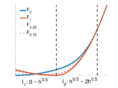
Further define
| (36) |
as a convex combination of and . Figure 3 gives a graphical sketch of , and . The key insight in the constructions of and is to use a cubic function to connect two quadratic functions of different curvatures, and hence allow to be the same on a wide region of (in particular ) and produce small difference . In contrast, the lower bound construction in existing work (Besbes et al., 2015) uses quadratic functions only, which are not capable of producing smooth functions that differ locally and therefore only applies to the special case of .
The following lemma lists some properties of . Their verification is left to Section B.5 in the online supplement.
Lemma B.3.
The following statements are true for all .
-
1.
satisfies (A1) through (A5) with , , , and .
-
2.
and .
-
3.
for all .
-
4.
.
We are now ready to describe our construction of a “hard” subset . Note that for all due to the monotonicity of (see Proposition 1.1). Therefore we shall focus solely on the case, whose construction is automatically valid for all .
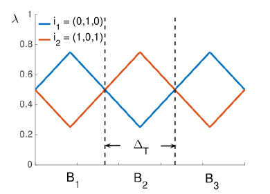
Let be a parameter to be determined later, and define . Again partition the entire time epochs into disjoint batches , where each batch consists of either or consecutive epochs. Let be the class of all binary vectors of length and let be a certain subset of to be specified later. The subset is constructed so that each function sequence is indexed by a unique -dimensional binary vector , with defined as
| (37) |
Figure 3 gives a visual illustration of the change pattern of and by plotting the values of for each function in the constructed sequences. For a particular batch , when then and are exactly the same within ; on the other hand, if then will drift towards the function and if the functions will drift towards , creating gaps between and within batch . For regularity reasons, we constrain the value to be within the range of regardless of values. We also note that and always agree on the first and the last epochs within each batch. This property makes repetition of constructions across all batches possible. The following lemma lists some key quantities of interest between and :
Lemma B.4.
Suppose for and for . For any consider and as defined in Eq. (37). Then the following statements are true:
-
1.
(Variation). , for all and .
-
2.
(Discrepancy). , where is the Hamming distance between and .
-
3.
(KL divergence). Let be the distribution of , with selected by an admissible policy . Then for any such policy we have that
Finally, we describe the construction of and the choices of and that give rise to matching lower bounds. For simplicity we restrict ourselves to being an even number. The construction of is based on the concept of constant-weight codings, where each code has exactly ones and zeros, and each pair of codes have large Hamming distance . The construction of constant-weight codings originates from (Graham & Sloane, 1980), and Wang & Singh (2016) gave an explicit lower bound on the size of , which we cite below:
Lemma B.5 (Wang & Singh (2016), Lemma 9).
Suppose and is even. There exists a subset such that , , and , . Furthermore, .
The univariate case of Theorem 3.2 can then be proved by appropriately setting the scalings of , and invoking Lemmas B.3, B.4 and B.5. Because and regret lower bounds for stationary stochastic online optimization are known (see, for example, (Hazan & Kale, 2014; Jamieson et al., 2012)), we only need to prove the lower bound with the additional assumption that for noisy gradient feedback and/or for noisy function value feedback . More specifically, for noisy gradient feedback we set , , and for noisy function feedback we set and . It is easy to verify that with the additional lower bound on , and , and therefore the constructions are valid. A complete proof is given in Sec. B.3 after we introduce our adversarial construction of , which includes the univariate setting () as a special case.
B.3 Extension to higher dimensions
The lower bound construction can be extended to higher dimensions to obtain a matching lower bound of for noisy gradient feedback and for noisy function value feedback. Let be a -dimensional vector with all components equal to . We consider . Define as follows:
| (38) |
Here is the univariate function defined in Eq. (36). Intuitively, the multi-variate function is constructed by “projecting” a -dimensional vector onto a 1-dimensional axis supported on , and subsequently invoking existing univariate construction of adversarial functions. An additional quadratic term is appended to ensure the strong convexity of without interfering with the structure in . The following lemma lists the properties of , which are rigorously verified in Section B.7 in the online supplement.
Lemma B.6.
Suppose . The following statements are true for any fixed and all .
-
1.
satisfies (A1) through (A5) with , , , and .
-
2.
and .
-
3.
for all .
-
4.
.
The third property in Lemma B.6 deserves special attention, which is a key property that is significantly different from Lemma B.3 for the univariate case, because the dependency of on has an extra term involving the domain dimension in the exponent. At a higher level, the presence of the term comes from the concentration of measure phenomenon in high dimensions.
We then have the next corollary, by following the same construction of in the univariate case and invoking Lemma B.6:
Corollary B.1.
Suppose is even, and . Let be constructed according to Lemma B.5, and , where is defined in Eq. (37) except that is replaced with its high-dimensional version defined in Eq. (38). Then the following holds:
-
1.
(Variation). for all , .
-
2.
(Discrepancy). .
-
3.
(KL-divergence). For all admissible policy , for and for .
We now prove the multi-dimensional case based on Corollary B.1. First consider the noisy gradient feedback . Set and accordingly such that . This yields and . The KL divergence is then upper bounded by and . By carefully selecting constants in the asymptotic notations, one can make the right-hand side of Eq. (28) to be lower bounded by 1/2. Subsequently invoking Lemma B.1, we conclude that there does not exist an admissible policy such that . The lower bound proof is then completed by the discrepancy claim in Corollary B.1 that .
The proof for the noisy function value feedback is similar. The only difference is that the KL divergence is upper bounded by , for which we should set that leads to and . We then have that and . Using the same argument, the regret for any admissible policy is lower bounded by .
B.4 Proof of Lemma B.1
Let be a policy that attains the minimax rate. By Markov’s inequality, with probability it holds that
| (39) |
Define , where is the (unique) minimizer of . Let and . Because minimizes the “empirical” regret on , it holds that
Subsequently,
Therefore, we must have conditioned on Eq. (39), which completes the proof.
B.5 Proof of Lemma B.3
We verify the properties separately.
Verification of property 1: (A1) is obvious because . We next focus (A3), (A4) and (A5). It is easy to check that if two functions and satisfy (A3) through (A5), then their convex combination for also satisfies (A3) through (A5). Therefore we only need to verify these conditions for and , respectively. We first prove that both and are differentiable. Because both and are differentiable within each piece, to prove the global differentiablity we only need to show that the left and right function values and derivatives of and at and are equal. Define , , and . We then have that , , , , , . Therefore, both and are differentiable on . It is then easy to check that and . Therefore (A3) is satisfied with .
To verify (A4) and (A5) we need to compute the second-order derivatives of and . By construction, for , for , and for . Therefore, and satisfy (A4) and (A5) with and . Note that and are not twice differentiable at and : however, this does not affect the smoothness and strong convexity of both functions.
Finally we check (A2). Let be the unique minimizer of . Elementary algebra yields that . Because , we know that satisfies (A2) with for .
Verification of property 2: It is easy to see that and for all . Thus we only need to consider and . It is easy to verify that and .
Verification of property 3: Similarly we only need to consider and . Because and only differ on , we have that
Verification of property 4: We have that and . Subsequently, .
B.6 Proof of Lemma B.4
Fix an arbitrary interval for some . Without loss of generality assume (the extra one function in some intervals can be safely neglected as both and are large). Then
Subsequently,
For the discrepancy term, again fix for some such that . We then have,
Subsequently, summing over all intervals with we have that .
Finally we compute the KL divergence . We first consider the noisy function value feedback . Let be the random variables of the feedbacks and denote and . For any admissible policy , we have that
Here the third identity holds because are independent. For , it holds that
| (40) |
where in the last inequality we invoke Lemma B.3. Summing over to we have that .
The noisy gradient feedback case can be handled by following the same argument, except that Eq. (40) should be replaced by
Therefore, .
B.7 Proof of Lemma B.6
We verify the properties separately.
Verification of property 1: Because , , we have that for all and therefore satisfies (A1) with .
We next verify (A3). Because is convex differentiable, it holds that is also convex differentiable because convexity is preserved with affine transform. In particular, and . Therefore, (A3) is satisfied with .
To verify (A4) and (A5), note that is twice differentiable except at points . Furthermore, . Subsequently, on points where is twice differentiable, we have that and . Therefore, (A4) and (A5) are satisfied with and .
Finally we check (A2). Let be the unique minimizer of on . It is clear that must take the form of , which gives the smallest without changing the value of . Completing the squares in we have that
| (41) |
Subsequently, . It is easy to verify that for , . Therefore, for all and the condition (A2) holds with .
Verification of property 2: . In addition, . Omitting the dependency on we obtain property 2.
Verification of property 3: Define . It is easy to verify that . Subsequently, for any we have that
Verification of property 4: From previous derivations we know that with and . Subsequently,
Appendix C Proof of Theorem 3.3
We give the proof of Theorem 3.3 that establishes an upper regret bound for functions that are merely convex; i.e., do not satisfy smoothness (A4) or strong convexity (A5). The meta-policy remains the same, and the sub-policy is also the OGD algorithm, but with a slightly different step size rule. The following lemma then upper bounds the regret against stationary benchmarks. It is a standard result in online convex optimization, whose proof can be found in, e.g., (Bubeck et al., 2012).
Lemma C.1.
Fix . Let be an arbitrary sequence of convex functions satisfying (A1) through (A3). For noisy gradient feedback and the OGD policy, the following holds with :
We next derive a decomposition of the strong regret and an affinity lemma, similar to Eq. (11) and Lemma 4.2. However, because strong convexity of is no longer assumed, it is technically challenging to upper bound as in Lemma 4.2. To overcome such difficulties, we gave an alternative decomposition of the strong regret, which can then be upper bounded for general convex functions.
For any sequence of convex functions let be the minimizer of . Then for any , the gap between strong and weak regret can be decomposed as
| (42) |
Here the second inequality holds because is the minimizer of , and therefore for all . We then have the following affinity lemma that upper bounds using .
Lemma C.2.
Suppose . Fix , and let be the minimizers of and , respectively. Then under (A1) through (A3) we have that
While Lemmas C.2 and 4.2 appear similar, their proofs are actually different. Unlike the proof of Lemma 4.2 that analyzes and uses the strong convexity of and in an essential way, in the proof of Lemma C.2 we directly analyze the behavior of and in a small neighborhood of (or without resorting to . Thus, Lemma C.2 works for non-smooth and non-strongly convex functions. We give the complete proof of Lemma C.2 in Sec. C.1.
Combining Lemmas C.1, C.2 and Eq. (42) we can prove the desired upper bound in Theorem 3.3 using the same analysis in the proof of Theorem 3.1. More specifically, we have
The critical parameter should then be set as if and otherwise.
C.1 Proof of Lemma C.2
Because of symmetry we only need to prove . Recall the definition for and the properties that , and .
Now set for some to be specified later. Because is Lipschitz continuous, we have for all . On the other hand, for all because is the minimizer of . Combining both inequalities we have
Here is a constant that only depends on and . Integrating both sides of the above inequality on and noting that , we have
Subsequently, Taking where we have . Because both and are uniformly bounded (thanks to assumption (A2)) on a compact domain , we have that and therefore the term is dominated by , because .
Appendix D Proofs of other technical propositions
D.1 Proof of Proposition 1.1
By monotonicity of -space, we know that for any measurable function ,
provided that integration on both sides of the inequality (or there limits) exist. Hence, for all and therefore .
By Hölder’s inequality, we know that for any -dimensional vector it holds that
| (43) |
where for and for is the norm of vector . Applying Eq. (43) on the -dimensional vector we have that
Multiplying both sides of the above inequality by we have that .
D.2 Proof of Proposition 3.1
References
- Abernethy et al. (2008) Abernethy, J., Hazan, E., & Rakhlin, A. (2008). Competing in the dark: An efficient algorithm for bandit linear optimization. In Proceedings of the Conference on Learning Theory (COLT).
- Agarwal et al. (2012) Agarwal, A., Bartlett, P. L., Ravikumar, P., & Wainwright, M. J. (2012). Information-theoretic lower bounds on the oracle complexity of stochastic convex optimization. IEEE Transactions on Information Theory, 58(5), 3235–3249.
- Agarwal et al. (2010) Agarwal, A., Dekel, O., & Xiao, L. (2010). Optimal algorithms for online convex optimization with multi-point bandit feedback. In Proceedings of Conference on Learning Theory (COLT).
- Agarwal et al. (2013) Agarwal, A., Foster, D. P., Hsu, D., Kakade, S. M., & Rakhlin, A. (2013). Stochastic convex optimization with bandit feedback. SIAM Journal on Optimization, 23(1), 213–240.
- Besbes et al. (2015) Besbes, O., Gur, Y., & Zeevi, A. (2015). Non-stationary stochastic optimization. Operations Research, 63(5), 1227–1244.
- Boyd & Vandenberghe (2004) Boyd, S., & Vandenberghe, L. (2004). Convex optimization. Cambridge university press.
- Bubeck et al. (2012) Bubeck, S., Cesa-Bianchi, N., et al. (2012). Regret analysis of stochastic and nonstochastic multi-armed bandit problems. Foundations and Trends® in Machine Learning, 5(1), 1–122.
- Bubeck et al. (2017) Bubeck, S., Eldan, R., & Lee, Y. T. (2017). Kernel-based methods for bandit convex optimization. In Proceedings of the Annual ACM SIGACT Symposium on Theory of Computing (STOC).
- Castro & Nowak (2008) Castro, R. M., & Nowak, R. D. (2008). Minimax bounds for active learning. IEEE Transactions on Information Theory, 54(5), 2339–2353.
- Cover & Thomas (2006) Cover, T., & Thomas, J. (2006). Elements of Information Theory. Wiley, 2 ed.
- Daniely et al. (2015) Daniely, A., Gonen, A., & Shalev-Shwartz, S. (2015). Strongly adaptive online learning. In International Conference on Machine Learning, (pp. 1405–1411).
- den Boer (2015) den Boer, A. V. (2015). Dynamic pricing and learning: Historical origins, current research, and new directions. Surveys in Operations Research and Management Science, 20(1), 1–18.
- den Boer & Zwart (2015) den Boer, A. V., & Zwart, B. (2015). Dynamic pricing and learning with finite inventories. Operations Research, 63(4), 965–978.
- Flaxman et al. (2005) Flaxman, A. D., Kalai, A. T., & McMahan, H. B. (2005). Online convex optimization in the bandit setting: gradient descent without a gradient. In Proceedings of the Annual ACM-SIAM symposium on Discrete algorithms (SODA).
- Graham & Sloane (1980) Graham, R., & Sloane, N. (1980). Lower bounds for constant weight codes. IEEE Transactions on Information Theory, 26(1), 37–43.
- Gur (2014) Gur, Y. (2014). Sequential Optimization in Changing Environments: Theory and Application to Online Content Recommendation Services. Ph.D. thesis, Columbia University.
- Hall & Willett (2015) Hall, E. C., & Willett, R. M. (2015). Online convex optimization in dynamic environments. IEEE Journal of Selected Topics in Signal Processing, 9(4), 647–662.
- Hazan (2016) Hazan, E. (2016). Introduction to online convex optimization. Foundations and Trends in Optimization, 2(3-4), 157–325.
- Hazan et al. (2007) Hazan, E., Agarwal, A., & Kale, S. (2007). Logarithmic regret algorithms for online convex optimization. Machine Learning, 69(2), 169–192.
- Hazan & Kale (2014) Hazan, E., & Kale, S. (2014). Beyond the regret minimization barrier: Optimal algorithms for stochastic strongly-convex optimization. Journal of Machine Learning Research, 15, 2489–2512.
- Hazan & Levy (2014) Hazan, E., & Levy, K. (2014). Bandit convex optimization: Towards tight bounds. In Proceedings of the Advances in Neural Information Processing Systems (NIPS).
- Ibragimov & Has’minskii (1981) Ibragimov, I. A., & Has’minskii, R. Z. (1981). Statistical Estimation: Asymptotic Theory. New York: Springer-Verlag.
- Jadbabaie et al. (2015) Jadbabaie, A., Rakhlin, A., Shahrampour, S., & Sridharan, K. (2015). Online optimization: Competing with dynamic comparators. In Artificial Intelligence and Statistics, (pp. 398–406).
- Jamieson et al. (2012) Jamieson, K. G., Nowak, R., & Recht, B. (2012). Query complexity of derivative-free optimization. In Proceedings of the Advances in Neural Information Processing Systems (NIPS).
- Karnin & Anava (2016) Karnin, Z. S., & Anava, O. (2016). Multi-armed bandits: Competing with optimal sequences. In Proceedings of the Advances in Neural Information Processing Systems (NIPS).
- Keskin & Zeevi (2017) Keskin, N. B., & Zeevi, A. (2017). Chasing demand: Learning and earning in a changing environment. Mathematics of Operations Research, 42(2), 277–307.
- McMahan (2017) McMahan, H. B. (2017). A survey of algorithms and analysis for adaptive online learning. Journal of Machine Learning Research, 18, 1–50. ArXiv preprint arXiv:1403.3465.
- Mokhtari et al. (2016) Mokhtari, A., Shahrampour, S., Jadbabaie, A., & Ribeiro, A. (2016). Online optimization in dynamic environments: Improved regret rates for strongly convex problems. In Decision and Control (CDC), 2016 IEEE 55th Conference on, (pp. 7195–7201). IEEE.
- Nesterov & Nemirovskii (1994) Nesterov, Y., & Nemirovskii, A. (1994). Interior-point polynomial algorithms in convex programming. SIAM.
- Raskutti et al. (2011) Raskutti, G., Wainwright, M. J., & Yu, B. (2011). Minimax rates of estimation for high-dimensional linear regression over -balls. IEEE Transactions on Information Theory, 57(10), 6976–6994.
- Saha & Tewari (2011) Saha, A., & Tewari, A. (2011). Improved regret guarantees for online smooth convex optimization with bandit feedback. In Proceedings of the International Conference on Artificial Intelligence and Statistics (AISTATS).
- Shamir (2015) Shamir, O. (2015). An optimal algorithm for bandit and zero-order convex optimization with two-point feedback. ArXiv preprint arXiv:1507.08752.
- Tsybakov (2009) Tsybakov, A. B. (2009). Introduction to nonparametric estimation.. Springer Series in Statistics. Springer, New York.
- Wang & Singh (2016) Wang, Y., & Singh, A. (2016). Noise-adaptive margin-based active learning and lower bounds under tsybakov noise condition. In Proceedings of the AAAI Conference on Artificial Intelligence (AAAI).
- Yu (1997) Yu, B. (1997). Assouad, fano, and le cam. In Festschrift for Lucien Le Cam, (pp. 423–435). Springer.
- Yudin & Nemirovskii (1983) Yudin, D., & Nemirovskii, A. (1983). Problem complexity and method efficiency in optimization. John Wiley and Sons.
- Zhang et al. (2017) Zhang, L., Yang, T., Jin, R., & Zhou, Z.-H. (2017). Strongly adaptive regret implies optimally dynamic regret. arXiv preprint arXiv:1701.07570.
- Zinkevich (2003) Zinkevich, M. (2003). Online convex programming and generalized infinitesimal gradient ascent. In Proceedings of the 20th International Conference on Machine Learning (ICML-03), (pp. 928–936).