On Euler’s inequality and
automated reasoning with dynamic geometry

Abstract

Euler’s inequality $R\geq 2r$ can be investigated in a novel way by using implicit loci in GeoGebra. Some unavoidable side effects of the implicit locus computation introduce unexpected algebraic curves. By using a mixture of symbolic and numerical methods a possible approach is sketched up to investigate the situation. By exploiting fast GPU computations, a web application written in CindyJS helps in understanding the situation even better.

1 GeoGebra: a symbolic tool for obtaining generalizations of geometric statements

GeoGebra [7] is a well known dynamic geometry software package with millions of users worldwide. Its main purpose is to visualize geometric invariants. Recently GeoGebra has been supporting investigation of geometric constructions also symbolically by harnessing the strength of the embedded computer algebra system (CAS) Giac [9]. One direct use of the embedded CAS is automated reasoning [10]. In this paper we use in particular the implicit locus derivation feature [1] in GeoGebra, by using the command LocusEquation with two inputs: a Boolean expression and the sought mover point. For example, given an arbitrary triangle $ABC$ with sides $a$, $b$ and $c$, entering LocusEquation[$a$==$b$,$C$] results in the perpendicular bisector $d$ of $AB$, that is, if $C$ is chosen to be an element of $d$, then the condition $a=b$ is satisfied.

Obtaining implicit loci is a recent method in GeoGebra to get interesting facts on classic theorems. These facts are closely related to algebraic curves which usually describe generalization of the classic results. Sometimes it is computationally difficult to obtain the curves quickly enough, but some new improvements in Giac’s elimination algorithm opened the road to effectively investigate a large number of geometric constructions [11, 12] including Holfeld’s 35th problem [11, 6], a generalization of the Steiner-Lehmus theorem [11, 14] or the right triangle altitude theorem [1].

We need to admit that the possibility to generalize well known theorems is a consequence of using unordered geometry [2, p. 97] in the applied tools and theories. In unordered geometry one cannot designate only one intersection point of a line and a conic (or two conics), so both will be considered at the same time. (See [2, p. 59] for an example on irreducible problems and undistinguishable cases.) Therefore we obtain a larger set of points for the resulting algebraic curve as expected. The obtained set may be inconvenient in some cases, but can be fruitful to get some interesting generalizations.

Finally we demonstrate a new approach in using the GPU of the user’s computer by utilizing CindyJS [5] that colors the points of the plane according to a predefined relationship. In this way we can have a numerical solution very quickly, however some CindyScript programming will be required.

2 Euler’s inequality

We recall that in Euclidean planar geometry Euler’s inequality states that $R\geq 2r$ where $R$ and $r$ denote the radius of the circumscribed circle and the inscribed circle of a triangle, respectively.

Since GeoGebra’s Automated Reasoning Tools [10] use Gröbner bases in the background, inequalities cannot really be investigated by them automatically. Certain experiments can however be started by fixing the ratio of the studied quantities, here $R$ and $r$. For example, one can start with some concrete experience by comparing $R$ and say $3r$ (see Fig. 1), and then simply change the constant $3$ to some different value. As output, the red curve in the figure gives a necessary geometric condition where to put $C$ in order to have $R=3r$.

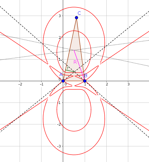
Figure 1: An implicit curve (in red) as the output of GeoGebra command LocusEquation[$R$==$3r$,$C$]. Here points $A$ and $B$ are fixed in the plane and $C$ is a free point. (In other words: Triangle $ABC$ has fixed vertices $A$ and $B$.) The computation of the sought set of mover point $C$ is a moderately difficult problem: an Intel(R) Core(TM) i7 CPU 860 @ 2.80GHz computer requires 3.7 seconds for the whole computation.

The result seems complicated for the first look. By doing some more experiments, it turns out that the two inner oval parts of the curve show relevant information on the concrete question, but the other parts show something different. That is, by setting $C$ to an arbitrary point of the inner oval parts, the equality $R=3r$ will occur. For the other parts we will see later in Sec. 2.2 that the radii $r_{a}$, $r_{b}$ and $r_{c}$ of the excircles will take the role of $r$ over.

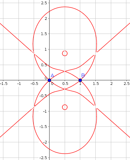
Figure 2: Result of LocusEquation[$R$==$2.1r$,$C$] and LocusEquation[$R$==$2.01r$,$C$]. To properly plot the latter a suitable zoom factor may be required due to possible inaccuracies in the plotting routine in GeoGebra.

After doing further experiments by changing the constant $3$ to lower values, when getting close to $2$ the inner oval parts seem to disappear even more and more (Fig. 2), and finally for the experiment $R=2r$ the inner oval parts are not visible any longer (Fig. 3).

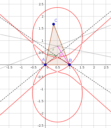
Figure 3: The inner oval parts disappear when plotting the case $R=2r$.

The first confusing result is why the points $\left(\frac{1}{2},\pm\frac{\sqrt{3}}{2}\right)$ are not plotted in this graph—we recall that the equality holds if and only if the triangle is equilateral. Unfortunately, the plotting routine in GeoGebra does not show this isolated point. In fact, other systems (including Wolfram$\mid$Alpha and Desmos) are also unable to automatically plot even the easiest examples of a very similar situation, namely that a curve has an acnode. Such a basic example is the curve $x^{3}-x^{2}-y^{2}=0$ for which the point $(0,0)$ is not shown in the graph, but is clearly an isolated point of the curve [17].

The result of the command LocusEquation[$R$==$2r$,$C$] is

$$x^{18}-225\;y^{18}-1481\;x^{2}\;y^{16}-4004\;x^{4}\;y^{14}-5460\;x^{6}\;y^{12}-3262\;x^{8}\;y^{10}+770\;x^{10}\;y^{8}+2604\;x^{12}\;y^{6}+1756\;x^{14}\;y^{4}+535\;x^{16}\;y^{2}-504\;x^{17}+1256\;x\;y^{16}+6752\;x^{3}\;y^{14}+13632\;x^{5}\;y^{12}+10336\;x^{7}\;y^{10}-4400\;x^{9}\;y^{8}-14304\;x^{11}\;y^{6}-11008\;x^{13}\;y^{4}-3808\;x^{15}\;y^{2}+1764\;x^{16}+1276\;y^{16}+1416\;x^{2}\;y^{14}-6936\;x^{4}\;y^{12}-11544\;x^{6}\;y^{10}+8608\;x^{8}\;y^{8}+33048\;x^{10}\;y^{6}+30104\;x^{12}\;y^{4}+11896\;x^{14}\;y^{2}-3528\;x^{15}-2888\;x\;y^{14}-2296\;x^{3}\;y^{12}+6296\;x^{5}\;y^{10}-7000\;x^{7}\;y^{8}-41944\;x^{9}\;y^{6}-47080\;x^{11}\;y^{4}-21368\;x^{13}\;y^{2}+4410\;x^{14}-1094\;y^{14}+2854\;x^{2}\;y^{12}-1262\;x^{4}\;y^{10}-370\;x^{6}\;y^{8}+31246\;x^{8}\;y^{6}+46226\;x^{10}\;y^{4}+24230\;x^{12}\;y^{2}-3528\;x^{13}-2888\;x\;y^{12}+592\;x^{3}\;y^{10}+5704\;x^{5}\;y^{8}-12704\;x^{7}\;y^{6}-29240\;x^{9}\;y^{4}-17840\;x^{11}\;y^{2}+1764\;x^{12}+1276\;y^{12}-1136\;x^{2}\;y^{10}-5940\;x^{4}\;y^{8}+1472\;x^{6}\;y^{6}+11604\;x^{8}\;y^{4}+8368\;x^{10}\;y^{2}-504\;x^{11}+1256\;x\;y^{10}+2984\;x^{3}\;y^{8}+912\;x^{5}\;y^{6}-2608\;x^{7}\;y^{4}-2296\;x^{9}\;y^{2}+63\;x^{10}-225\;y^{10}-581\;x^{2}\;y^{8}-330\;x^{4}\;y^{6}+246\;x^{6}\;y^{4}+283\;x^{8}\;y^{2}=0.$$

By using GeoGebra’s Substitute[$I$,{$x$=1/2,$y$=sqrt(3)/2}] command (here $I$ denotes the obtained implicit curve object) we get $0=0$ which shows that the expected point is indeed an element of the curve. The same result can be seen for the point $\left(\frac{1}{2},-\frac{\sqrt{3}}{2}\right)$.

The obtained polynomial can be factored by using GeoGebra’s Factor[LeftSide[$I$]-RightSide[$I$] command. The factorization is

$$\left(x^{2}+y^{2}\right)\;\cdot\;\left(7\;x^{8}-28\;x^{7}+12\;x^{6}\;y^{2}+42\;x^{6}-36\;x^{5}\;y^{2}-28\;x^{5}-6\;x^{4}\;y^{4}+34\;x^{4}\;y^{2}+7\;x^{4}+12\;x^{3}\;y^{4}-8\;x^{3}\;y^{2}-20\;x^{2}\;y^{6}-26\;x^{2}\;y^{4}-2\;x^{2}\;y^{2}+20\;x\;y^{6}+20\;x\;y^{4}-9\;y^{8}+46\;y^{6}-9\;y^{4}\right)\;\cdot\;\left(9\;x^{8}-36\;x^{7}+52\;x^{6}\;y^{2}+54\;x^{6}-156\;x^{5}\;y^{2}-36\;x^{5}+102\;x^{4}\;y^{4}+190\;x^{4}\;y^{2}+9\;x^{4}-204\;x^{3}\;y^{4}-120\;x^{3}\;y^{2}+84\;x^{2}\;y^{6}+186\;x^{2}\;y^{4}+34\;x^{2}\;y^{2}-84\;x\;y^{6}-84\;x\;y^{4}+25\;y^{8}-14\;y^{6}+25\;y^{4}\right).$$

Here the first factor $p_{1}=x^{2}+y^{2}$ clearly corresponds to the point $A$. The second factor $p_{2}=7x^{8}-\ldots$ shows all real points of the curve $I$ (without the points $\left(\frac{1}{2},\pm\frac{\sqrt{3}}{2}\right)$), and the third factor $p_{3}=9x^{8}-\ldots$ has seemingly no real points, but after computing its acnodes by solving the inequality system $p_{3}=0$, $(p_{3})^{\prime}_{x}=0$, $(p_{3})^{\prime}_{y}=0$, $H(p_{3})>0$, where $H$ denotes the Hessian matrix, we may explore symbolically that the polynomial indeed describes the two expected isolated real points as well.

This approach with the Hessian cannot be achieved in GeoGebra. Instead, a numerical way can be tried to visualize the function $f(x,y)=p_{3}$ in 3 dimensions (Fig. 4) to find the real roots, namely $\left(\frac{1}{2},\pm\frac{\sqrt{3}}{2}\right)$, $(0,0)$ and $(1,0)$. Also in some other computer algebra systems a contour plot may help (see Fig. 5), or to use extra packages which have more sophistical methods to plot real curves (as seen in Fig. 6).

Finally we remark that by using Maple’s evala(AFactor($\ldots$)) command we can verify that $p_{2}$ and $p_{3}$ are irreducible over $\mathbb{C}$. This can also be achieved by using Singular’s absolute factorization library (absfact_lib).

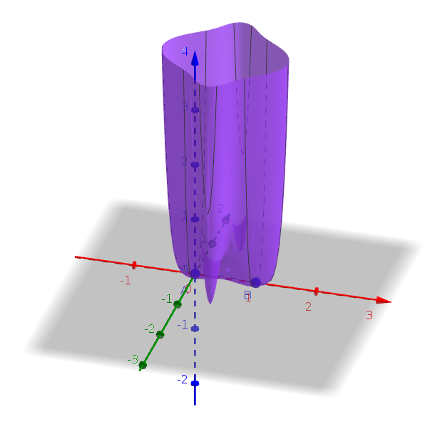
Figure 4: A 3D plot of $p_{3}$ in GeoGebra. Here we used the command $f(x,y):=$Element[Factors[LeftSide[$I$]-RightSide[$I$]],3,1] and opened the Graphics 3D View.

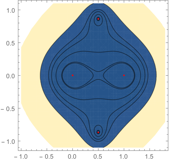
Figure 5: A contour plot of $p_{3}$ in Mathematica.

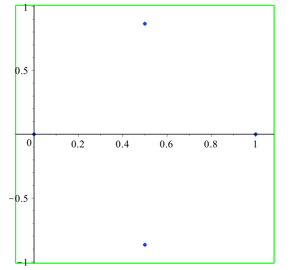
Figure 6: Plotting $p_{3}$ with Maple’s algcurves package and its plot_real_curve command.

2.1 Summary of the difficulties

The above shows some difficulties in our case. First of all, by using Gröbner bases there seems no completely automatic way to obtain Euler’s inequality—however, the paper [4] sketches up a possible method (without full explanation in general). In our approach one needs to start some experiments by choosing the ratio between $R$ and $r$ randomly. In our opinion, this problem can be automatically resolved by using real geometry and quantifier elimination [3] not only in our case, but in general (see [16] for some details).

The second problem is that the plotted graph can be inaccurate: the equilateral case for $R=2r$ cannot be read off by the user in GeoGebra. It would be expected that the output curve should contain the set of points where the equality holds—this does not seem to be the case here because of the failure of the plotting algorithm. The case of failure even for some easy cubic examples show that this problem cannot be easily worked around without using extra software packages.

For similar reasons the factorization does not directly help finding the equilateral case, either. Only a 3D plot—actually a numerical approach—gives some hints where to look for the equality.

2.2 Why the octic $p_{2}$?

Similarly to the Steiner-Lehmur generalization in [14] here we silently introduced three other circles as extensions of the incircle. They are the excircles—in unordered geometry one cannot distinguish between internal and external angle bisectors. (See also [2, p. 60] for a discussion on this.)

After some experimenting it can be concluded that different sections of the octic $p_{2}$ describe different circles among the three excircles (Fig. 7).

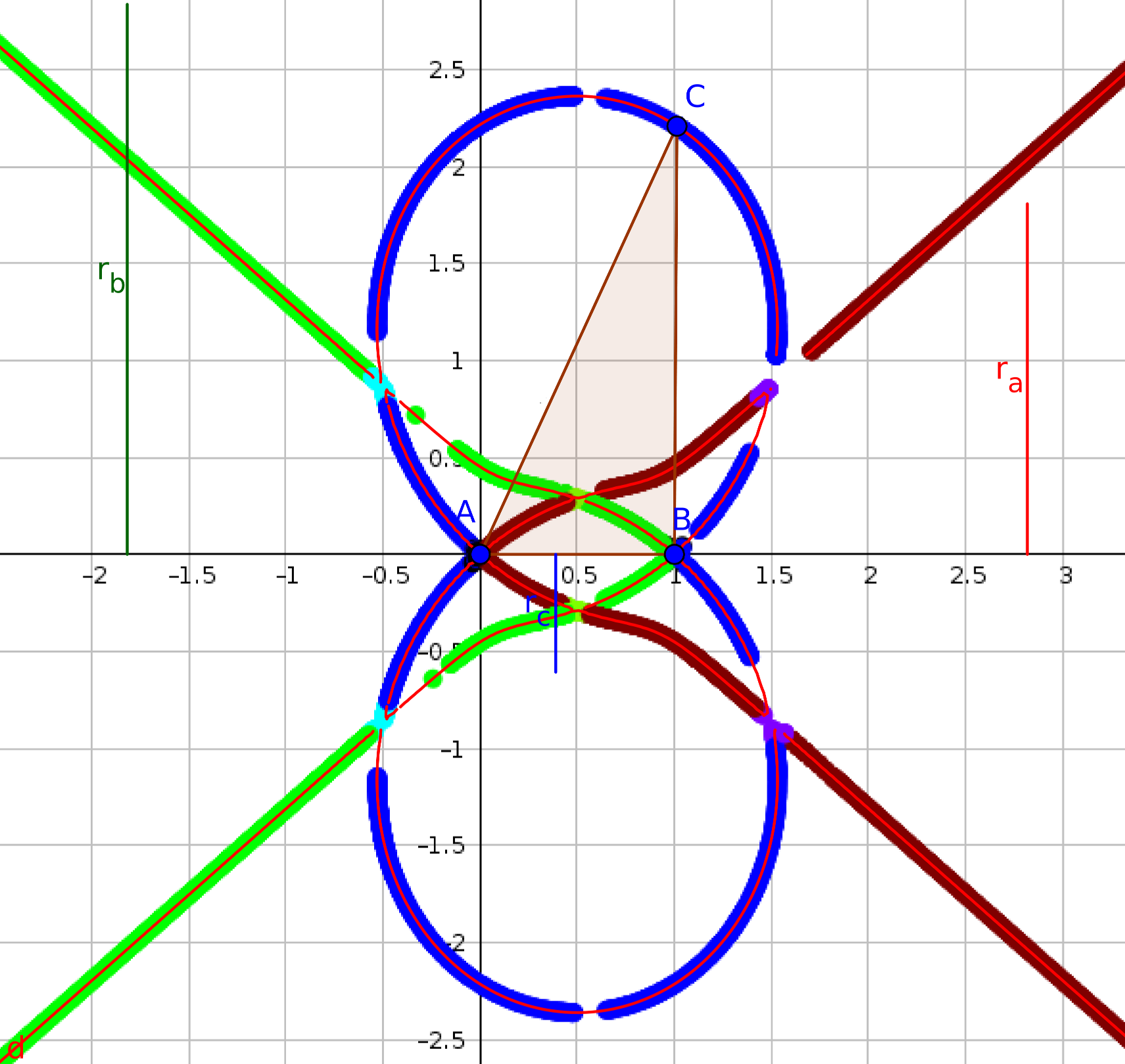
Figure 7: Various parts of the octic $p_{2}$ show the sought moving points $C$ for statements $R=2r_{a}$ (red), $R=2r_{b}$ (green) and $R=2r_{c}$ (blue). The figure was produced with GeoGebra by attaching a new point (denoted again by $C$) to the octic $p_{2}$, and then constructing $r_{a}$, $r_{b}$, $r_{c}$ and $R$ by using the attached point as “$C$”, and computing which excircle would be connected with the appropriately chosen attached point—then the color of $C$ was dynamically set by using the RGB scheme (see [13] for a similar concept). Finally tracing and animation were switched on for $C$ to cover all possible screen points of the octic.

2.3 The inequality does not hold for excircles

Continuing the process that changing the constant $3$ to lower values, including less numbers than $2$, we learn that the inner oval parts of the curve will not be visible any longer. This is the case e. g. for $1.9$: there are no visible inner oval parts (and they do not exist, either, because of Euler’s inequality), but the other parts still do (Fig. 8). This supports the idea that the inequality with respect to $r$ cannot be transferred to $r_{a}$, $r_{b}$ or $r_{c}$. That is, we concluded that Euler’s inequality always fails on excircles.

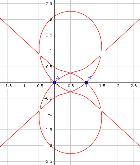
Figure 8: Result of LocusEquation[$1.9r$==$R$,$C$].

3 Another numerical approach: CindyJS

CindyJS [5] is a JavaScript library and built on top of the NodeJS infrastructure. It is designed to be able to load dynamic geometry files produced by Cinderella [8] in the long term. The plugin CindyGL utilizes the WebGL subsystem of the user’s web browser and gives direct access to the GPU to exploit fast computations. As a result various mathematical formulas can be investigated in a real-time way to get immediate feedback on the changing input when the user drags input points, for example. CindyJS has been developed by a team of computer graphics and dynamic geometry experts under the leadership of the Technical University of Munich, Germany.

By using a web browser and its access to the GPU a user can do fast visualization of the above properties. The following program code, shown and explained in shorter parts, is capable to use the vertices of a triangle $ABC$ as input, and then compute its radius $r$ and $R$ of the incircle and the circumcircle, respectively. Finally a contour plot is drawn to classify points of the plain with respect to the ratio $R/r$ in case the given point of the plane is chosen as $C$.

⬇

angularbisectors(P, Q, R) := (

p = complex(P);

q = complex(Q);

r = complex(R);

w = sqrt((r-p)*(q-p));

join(P, gauss(p+w));

);

The function angularbisectors returns the internal bisector of $\angle QPR$. The command gauss converts a complex number to a point and the command join connects its input points to represent the result as a line—this last command will be returned by the function.

To compute the distance from point $P$ to line $l$ we use the function

⬇

dist(P, l) := |P_1*l_1+P_2*l_2+P_3*l_3|/(|(l_1,l_2)|*|P_3|);

We also need to create the perpendicular bisector of the input points $P$ and $Q$:

⬇

perpbisector(P, Q):= (

p = complex(P);

q = complex(Q);

mid = (p+q)/2;

join(gauss(mid), gauss(mid+i*(q-p)))

);

Now we are ready to map a color to each point of the plane. We assume that for all $C$ points in the plane the function $f$ is to be used:

⬇

f(C) := (

b1 = angularbisectors(A, B, C);

b2 = angularbisectors(B, C, A);

incenter = meet(b1, b2);

r = dist(incenter, join(A, B));

p1 = perpbisector(A, B);

p2 = perpbisector(B, C);

circumcenter = meet(p1, p2);

R = |circumcenter.xy - A.xy|;

levels = 30;

floor(0.01/(R/r-2)*levels)/levels;

);

Here meet computes the intersection point of the input lines. After computing the values of $r$ and $R$ the final command designates the returned color for each input point $C$ by computing a numerical contour plot.

Finally we use the colorplot function with the running variable # that stands for all possible values of $C$ in the plane:

⬇

colorplot(exp(-2*|f(#)|));

To show only one particular value of $C$, that is, the current value that is based on the position of the point $C$ in the triangle being shown, we simply use

⬇

f(C);

and thereafter we will be able to draw the incircle and the circumcircle and print their radii on the screen:

⬇

drawcircle(incenter, r, color->[0,1,0]);

drawtext(incenter, "r = " + r, color->[0,1,0]);

drawcircle(circumcenter, R, color->[1,0,0]);

drawtext(circumcenter, "R = " + R, color->[1,0,0]);

drawtext(C, "R/r = " + R/r, color->[1,.5,0], align->"right");

The output of the code can be seen in Fig. 9. It is immediately clear that the ratio $R/r$ has an extremum in the “black area” of the figure. The black layer corresponds to ratios between $2$ and $2+\varepsilon$, the next level (that is a little bit lighter) corresponds to ratios between $2+\varepsilon$ and $2+2\varepsilon$, and so on. The value of $\varepsilon$ can be fine tuned at the end of the declaration of f(C) above.

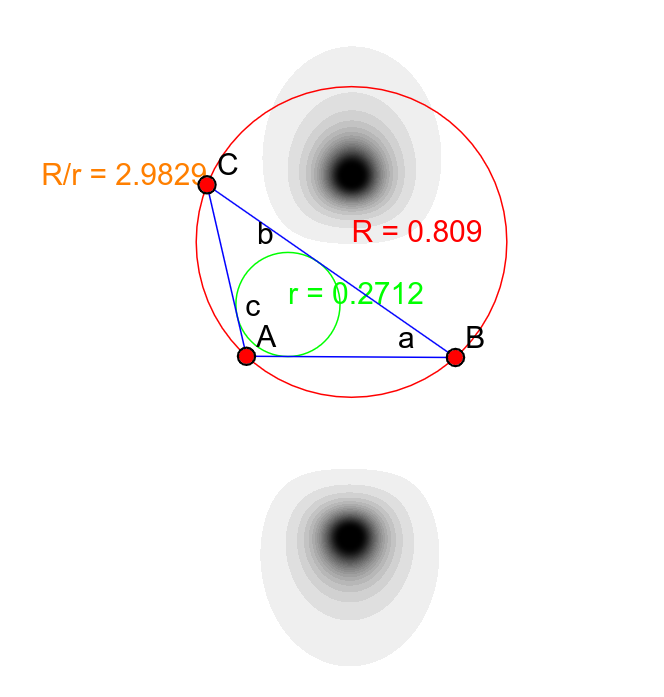
Figure 9: Output of CindyJS.

We highlight that the output can be better observed when points $A$ and $B$ are dragged. In this way we can “zoom in” the figure and have a more detailed understanding on the geometry of Euler’s inequality.

The full source code of this example can be found at github.com/CindyJS/CindyJS/blob/master/examples/cindygl/63_eulerinequality.html. On further details on programming CindyJS we refer to [15].

4 Conclusion

We used a novel method to obtain implicit loci in GeoGebra to investigate Euler’s inequality. This well known statement can also be approached by a mixture of symbolic and numerical observations. Our experiments are clearly not acceptable as a new way of proof, but steps to claim promising conjectures. For other investigations of classic or new statements—that is, to generalize geometric equations or inequalities—this kind of approach may be hopefully fruitful.

Also we highlight that a better approach might be to use real geometry and quantifier elimination. To find the most efficient way to formalize and prove Euler’s inequality and present it in an adequate form in a dynamic geometry software tool is an on-going work of the authors.

As a final comment we demonstrated how Euler’s inequality can be observed by using a new tool, namely CindyJS. Here we had to write a few lines of program code.

5 Acknowledgments

The authors thank Tomás Recio for his helpful comments on the first version of this paper.

The first author was partially supported by a grant MTM2017-88796-P from the Spanish MINECO (Ministerio de Economia y Competitividad) and the ERDF (European Regional Development Fund).

References

- [1] Abánades, M., Botana, F., Kovács, Z., Recio, T., Sólyom-Gecse, C.: Development of automatic reasoning tools in GeoGebra. ACM Commun. Comput. Algebra 50 (2016) 85–88
- [2] Chou, S.C.: Mechanical geometry theorem proving. Kluwer Academic Publishers Norwell, MA, USA (1987)
- [3] Collins, G.E., Hong, H.: Partial Cylindrical Algebraic Decomposition for quantifier elimination. Journal of Symbolic Computation 12(3) (1991) 299–328
- [4] Dalzotto, G., Recio, T.: On protocols for the automated discovery of theorems in elementary geometry. Journal of Automated Reasoning 43 (2009) 203–236
- [5] von Gagern, M., Kortenkamp, U. Richter-Gebert, J., Strobel, M.: CindyJS. Mathematical Visualization on Modern Devices. In: G. M. Greuel, T. Koch T., P. Paule, A. Sommese (eds), Mathematical Software – ICMS 2016. Lecture Notes in Computer Science, vol 9725. Springer, Cham (2016)
- [6] Hašek, R., Kovács, Z., Zahradník, J.: Contemporary interpretation of a historical locus problem with the use of computer algebra. In: Kotsireas, I.S., Martínez-Moro, E., eds.: Applications of Computer Algebra: Kalamata, Greece, July 20–23 2015. Volume 198 of Springer Proceedings in Mathematics & Statistics. Springer (2017)
- [7] Hohenwarter, M.: GeoGebra: Ein Softwaresystem für dynamische Geometrie und Algebra der Ebene. Master’s thesis, Paris Lodron University, Salzburg, Austria (2002)
- [8] Kortenkamp, U.: Foundations of dynamic geometry. Doctoral Thesis, ETH Zürich (1999)
- [9] Kovács, Z., Parisse, B.: Giac and GeoGebra – improved Gröbner basis computations. In Gutierrez, J., Schicho, J., Weimann, M., eds.: Computer Algebra and Polynomials. Lecture Notes in Computer Science. Springer (2015) 126–138
- [10] Kovács, Z., Recio, T., Vélez, M.P.: gg-art-doc (GeoGebra Automated Reasoning Tools. A tutorial). A GitHub project (2017) https://github.com/kovzol/gg-art-doc.
- [11] Kovács, Z.: Real-time animated dynamic geometry in the classrooms by using fast Gröbner basis computations. Mathematics in Computer Science 11 (2017)
- [12] Kovács, Z.: Achievements and Challenges in Automatic Locus and Envelope Animations in Dynamic Geometry. Mathematics in Computer Science (2018) https://doi.org/10.1007/s11786-018-0390-0
- [13] Losada, R.: El color dinámico en GeoGebra. La Gaceta de la Real Sociedad Matemática Española 17 (2014)
- [14] Losada, R., Recio, T., Valcarce, J.L.: On the automatic discovery of Steiner-Lehmus generalizations. In: Proceedings of ADG’2010, Lecture Notes in Computer Science. Springer, München (2010) 171–174
- [15] Montag, A., Richter-Gebert, J.: Bringing Together Dynamic Geometry Software and the Graphics Processing Unit. arXiv:1808.04579 (2018)
- [16] Robu, J.: Automated Proof of Geometry Theorems Involving Order Relation in the Frame of the Theorema Project. In: Proceedings of the International Conference on Knowledge Engineering, Principles and Techniques (KEPT2007), Cluj-Napoca, Romania (2007) 307–315
- [17] Wikipedia: Acnode — Wikipedia, the free encyclopedia (2016) [Online; accessed 10-July-2017].