Chiral liquid phase of simple quantum magnets

Abstract

We study a $T=0$ quantum phase transition between a quantum paramagnetic state and a magnetically ordered state for a spin $S=1$ XXZ Heisenberg antiferromagnet on a two-dimensional triangular lattice. The transition is induced by an easy plane single-ion anisotropy $D$. At the mean-field level, the system undergoes a direct transition at a critical $D=D_{c}$ between a paramagnetic state at $D>D_{c}$ and an ordered state with broken U(1) symmetry at $D<D_{c}$. We show that beyond mean field the phase diagram is very different and includes an intermediate, partially ordered chiral liquid phase. Specifically, we find that inside the paramagnetic phase the Ising ($J_{z}$) component of the Heisenberg exchange binds magnons into a two-particle bound state with zero total momentum and spin. This bound state condenses at $D>D_{c}$, before single-particle excitations become unstable, and gives rise to a chiral liquid phase, which spontaneously breaks spatial inversion symmetry, but leaves the spin-rotational U(1) and time-reversal symmetries intact. This chiral liquid phase is characterized by a finite vector chirality without long range dipolar magnetic order. In our analytical treatment, the chiral phase appears for arbitrarily small $J_{z}$ because the magnon-magnon attraction becomes singular near the single-magnon condensation transition. This phase exists in a finite range of $D$ and transforms into the magnetically ordered state at some $D<D_{c}$. We corroborate our analytic treatment with numerical density matrix renormalization group calculations.

I Introduction

Broken symmetries are ubiquitous in nature. Many broken-symmetry states have conventional long-range orders, such as dipolar magnetism or charge/orbital order, but some have more complex composite orders with order parameters built out of non-linear combinations of the original spin degrees of freedom. An example of such order is a spin nematic, whose order parameter is a bilinear combination of spin operators  Andreev and Grishchuk (1984); Chubukov (1990a); Penc and Läuchli (2011). Bilinear order parameters often emerge in frustrated spin systems, such as $J_{1}$-$J_{2}$-$J_{3}$ Heisenberg model on a square lattice Chandra et al. (1990a, b); Capriotti and Sachdev (2004), and describe spontaneous breaking of a discrete lattice rotational symmetry while spin-rotational SU(2) symmetry remains unbroken.

One of the first studies of composite orders was performed by Villain Villain (1977), who considered helical (spiral) spin order in Heisenberg and XY spin models in an external magnetic field ${\bm{h}}=h{\hat{\bm{z}}}$. He noticed that a helical order breaks both continuous and discrete symmetries. The continuous symmetry breaking corresponds to the development of a conventional dipolar magnetic order in the direction perpendicular to the field, i.e., to a finite expectation value $\langle{\bm{S}^{x,y}_{\bm{n}}}\rangle$ of the spin operator at every site of the lattice. The discrete symmetry breaking distinguishes between clockwise and anticlockwise rotations of spins from site ${\bm{n}}$ to site ${\bm{m}}$ along the bond $\langle{\bm{n}},{\bm{m}}\rangle$. Such an order is chiral in nature and the corresponding order parameter, vector chirality, is the $z$ component of the vector product of spins on a given bond ${\kappa}_{\bm{nm}}={\hat{\bm{z}}}\cdot{\bm{S_{n}}}\times\bm{S_{m}}$.

The fact that both continuous and discrete symmetries are broken in the ordered phase ($\langle\bm{S_{n}}\rangle\neq 0$ and $\langle\kappa_{\bm{nm}}\rangle\neq 0$) opens up a possibility of a sequence of phase transitions between this phase and the paramagnetic one, where $\langle\bm{S_{n}}\rangle=0$ and $\langle\kappa_{\bm{nm}}\rangle=0$. In the context of classical helimagnetism, Villain argued Villain (1977, 1978) that $\langle\bm{S_{n}}\rangle$ and $\langle\kappa_{\bm{nm}}\rangle$ do not need to acquire finite values simultaneously and that the paramagnetic and the magnetically ordered phases may be separated by the novel chiral liquid (CL) phase, in which the chiral order parameter is finite, i.e. $\langle\kappa_{\bm{nm}}\rangle\neq 0$, but long-range magnetic order is absent ($\langle\bm{S_{n}}\rangle=0$). A similar set of ideas has been recently applied to itinerant electron systems featuring various nematic orders Fradkin et al. (2010); Fernandes et al. (2012).

For thermodynamic phase transitions in U(1)-symmetric systems, the CL is expected to exist in a finite-temperature window $T_{\rm mag}<T<T_{\rm ch}$, where $T_{\rm ch}$ is the onset temperature of long-range chiral order and $T_{\rm mag}$ is the onset temperature of long-range magnetic order (Berezinskii-Kosterlitz-Thouless quasi-long-range order in two dimensions). Numerous numerical studies of two-dimensional classical helimagnets  Kawamura (1998); Hasenbusch et al. (2005); Korshunov (2006); Sorokin and Syromyatnikov (2012); Schenck et al. (2014) have found that $T_{\rm ch}$ and $T_{\rm mag}$ are indeed different, but the relative difference is very small, at best only a few percent.

Here, we consider a quantum phase transition at $T=0$ in systems with U(1) spin symmetry, driven by quantum fluctuations Sachdev (2001). Our goal is to understand whether a CL state can emerge as the ground state of the quantum spin system, separating a quantum paramagnet from a magnetically ordered phase. We argue below that the minimal model that describes this physics is a spin-1 triangular lattice XXZ antiferromagnet with nearest-neighbor exchange $J$ and single-ion anisotropy $D$. We find that CL phase exists in a rather wide range of $D$, whose width can be as large as $J/2$.

Our key result is presented in Fig. 1. It shows that a featureless paramagnetic state, realized at $D\gg J$, is separated from the magnetically ordered XY state at $D\ll J$ by the intermediate CL phase, which is stable in the finite window $D_{c}<D<D_{c}^{b}$.

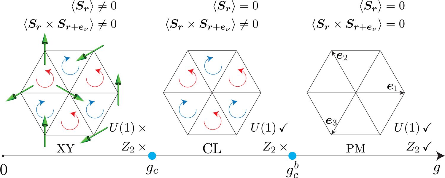
Figure 1: A schematic plot of the three phases {XY, CL, PM} as a function of the tuning parameter $g$, where $g\sim D/J$ for the quantum spin-1 model considered in this paper. For similar sequence of transitions in classical models $g\sim T$. The symmetries of each phase are noted on the bottom right of each hexagon.

In more specific terms, we analyzed the effects of magnon-magnon interaction in the paramagnetic phase. There are two gapped magnon modes in this phase. Their dispersion has minima at $\pm{\bm{Q}}$, where ${\bm{Q}}=(4\pi/3,0)$. Within self-consistent mean-field theory, magnon excitations soften at these momenta at $D_{c}\approx 2.68J$, and at smaller $D$ the system has an XY long-range spiral magnetic order, which breaks continuous U(1) symmetry (long-range magnetic order) and discrete $Z_{2}$ (chiral symmetry, spatial inversion, or parity). We found that the interaction between magnons with opposite spins is attractive. This attraction leads to the formation of a pair condensate of two magnons with zero total spin and zero total momentum, while individual magnon momenta are near $\pm{\bm{Q}}$. The attraction comes from the Ising, $J_{z}$, part of the exchange interaction, and involves both “normal” interaction terms with two creation and two annihilation magnon operators and “anomalous” interaction terms which do not conserve magnon numbers. The pairs condense at $D=D^{b}_{c}>D_{c}$, when single-magnon excitations are still gapped. The condensation gives rise to a finite staggered vector chirality $\kappa\neq 0$ for each elementary triangle of spins (up- and down-pointing triangles have opposite chirality). This CL state spontaneously breaks spatial inversion (parity) symmetry but preserves the time-reversal and translational symmetries because each unit cell includes one up-pointing and one down-pointing triangle.

The width of the chiral phase depends on the value of $J_{z}$. In our perturbative treatment, we found that there is no threshold of $J_{z}$, i.e., CL state develops for arbitrary small $J_{z}$ because the pairing interaction is singular at $D=D_{c}$. This singularity appears at second order in $J_{z}$ due to strong quantum renormalization of the interaction between magnons. Known from the previous renormalization group analysis, this spontaneous breaking of continuous U(1) and discrete $Z_{2}$ symmetries would become weakly first order, leading to a small but finite critical $J_{z}$ Kamiya et al. (2011); Parker and Balents (2017).

The paper is organized as follows. In Sec. II we introduce the model (Sec. II.1) and consider a toy problem of a single two-spin bound state (Sec. II.2). In Sec. III we introduce Schwinger bosons and solve for the two-magnon bound state in a many-body system in the presence of quantum fluctuations. We first present self-consistent analysis of single-magnon excitations and find the critical $D_{c}$. (Sec. III.1). Then, we derive the interaction between low-energy magnons (Sec. III.2), and show (Sec. III.3) that it is attractive in the channel, where the condensation of a two-magnon bound state leads to vector chirality. We solve for the two-magnon bound state first at small $J_{z}$ (Sec. III.4), to order $J^{2}_{z}$, and then for a generic $J_{z}$ (Sec. III.5). In Sec. IV we present DMRG calculations, which support our analytical results. In Sec. V we summarize our findings and outline their connections with other physical systems of current interest. In Appendix A we discuss two other phases in the vicinity of the CL phase: an Ising spin-density wave state and a supersolid (SS) state. In Appendix B we present the analysis of the bound-state development using an alternative procedure to relate spin operators to bosons.

Relation to earlier works. The separation between the breaking of a continuous and a discrete symmetry, either in classical (thermodynamic) or in quantum phase transitions, has been discussed for various physical problems. Several Heisenberg spin models on a square lattice, e.g., $J_{1}$-$J_{2}$ model, Ref. Chandra et al. (1990a, b), and $J_{1}$-$J_{3}$ model, Ref. Capriotti and Sachdev (2004), display $T=0$ order which breaks not only the SU(2) spin-rotational symmetry, but also a discrete lattice rotational symmetry. Thus, the ground state of the $J_{1}$-$J_{2}$ model at large $J_{2}$ is a stripe order with ferromagnetic spin arrangement either along $X$ or along $Y$ spatial direction. The order parameter associated with the difference between $X$ and $Y$ directions (an Ising nematic order) is quadratic in the spin operators  Chandra et al. (1990a). In two dimensions (2D), spin-rotational symmetry cannot be broken at any finite temperature $T\neq 0$, so that $\langle{\bm{S}}\rangle=0$, but the discrete $C_{\rm 4}$ lattice rotational symmetry breaks spontaneously down to $C_{\rm 2}$ below a certain Ising transition temperature $T_{\rm{Ising}}$. This leads to a finite-temperature liquid nematic phase with broken $Z_{2}$ symmetry. This has been identified in numerical studies Weber et al. (2003); Capriotti and Sachdev (2004).

In three dimensions (3D), long-range magnetic order $\langle{\bm{S}}\rangle\neq 0$ is present below Néel temperature $T<T_{N}$, but still there exists a temperature interval $T_{N}<T<T_{\rm{Ising}}$ where only a nematic order is present. For itinerant fermion systems, these ideas formed the basis Fernandes et al. (2012) for the magnetic scenario of the nematic order, observed in Fe-based superconductors.

In one-dimensional(1D) systems, continuous symmetries are preserved even at $T=0$ because of the singular nature of quantum fluctuations Sachdev (2001). There have been several studies of composite vector chiral (VC) orders at $T=0$. A spin chiral order with orbiting spin currents was found in $S=1/2$ two-leg zigzag Heisenberg spin ladder with XXZ-type exchange interaction Nersesyan et al. (1998). For an isotropic Heisenberg spin chain with competing interactions, it was shown Kolezhuk and Vekua (2005) that an external magnetic field acts in the same way as an exchange anisotropy and stabilizes long-ranged chiral order Chubukov (1991); Hikihara et al. (2008). A chiral order has been also found in a two-leg fully frustrated Bose-Hubbard ladder Dhar et al. (2013) and was argued to generate staggered orbital currents circling around elementary plaquettes Nersesyan (1991); Fjærestad and Marston (2002). Chiral phases have also been observed in $S=1$ zig-zag ladder Hikihara et al. (2001); Greschner et al. (2013). Magnetically-ordered states coexisting with chiral orders have also been studied at $T=0$ in triangular Momoi et al. (1997); Chubukov and Starykh (2013) and kagomé Domenge et al. (2005) geometries.

As described above, a VC order ${\kappa}_{\bm{nm}}\neq 0$ spontaneously breaks parity (a symmetry with respect to spatial inversion), but preserves time-reversal symmetry. This makes VC order, which is the topic of our study, very different from scalar chiral order $\chi_{\bm{nml}}=\bm{S_{n}}\cdot\bm{S_{m}}\times\bm{S_{l}}$ (where sites ${\bm{n}},{\bm{m}}$ and ${\bm{l}}$ form, e.g., a triangular plaquette). Such an order breaks both parity and time-reversal symmetries Wen et al. (1989). A ground state with a scalar chiral order without usual long-ranged magnetic order was proposed at the beginning of high-$T_{\rm c}$ era by Kalmeyer and Laughlin Kalmeyer and Laughlin (1987, 1989), who used a quantum-Hall-like incompressible bosonic wave function to describe it. In close analogy with the quantum Hall effect, this chiral spin state has gapped excitations in the bulk but gapless excitations at the edge of a sample. After almost 20 years this proposal has received a confirmation in a series of recent analytical and numerical studies of $S=\frac{1}{2}$ antiferromagnets Schroeter et al. (2007); Yao and Kivelson (2007); Thomale et al. (2009); Gong et al. (2014); Zhu et al. (2014); He et al. (2014); He and Chen (2015); Zhu et al. (2015).

Chiral (noncentrosymmetric) itinerant helimagnets have been found to exhibit a first-order thermodynamic phase transition into a chiral liquid phase that preempts the onset of magnetic ordering Tewari et al. (2006). While this phase does not break the chiral symmetry spontaneously, it shows that the chiral susceptibility can diverge while the magnetic susceptibility is still finite.

Our finding of the two-dimensional CL phase with finite vector chirality and no dipolar magnetic order is a realization of the composite VC order in the ground state of a two-dimensional quantum spin model.

II Anisotropic $S=1$ Triangular Antiferromagnet

II.1 Spin-1 model

We consider $S=1$ model on a triangular lattice, with anisotropic XXZ antiferromagnetic exchange between nearest neighbors and an easy-plane single-ion anisotropy, $D(S^{z})^{2}$, with $D>0$. This is the minimal model to study a quantum phase transition between a quantum paramagnet and a magnetically ordered state with an additional discrete symmetry breaking. Despite simplicity, the model describes real materials Zapf et al. (2006, 2014).

The Hamiltonian of the model is

$${\cal H}=\sum_{{\bm{r}},\nu,\mu}J_{\mu}S^{\mu}_{\bm{r}}S^{\mu}_{{\bm{r}}+{\bm{e}}_{\nu}}+D\sum_{{\bm{r}}}(S^{z}_{{\bm{r}}})^{2},$$ (1)

where ${\bm{e}}_{1}=a{\hat{\bm{x}}}$, ${\bm{e}}_{2}=a(-{\hat{\bm{x}}}/2+\sqrt{3}{\hat{\bm{y}}}/2)$ and ${\bm{e}}_{3}=a(-{\hat{\bm{x}}}/2-\sqrt{3}{\hat{\bm{y}}}/2)$ (see Fig. 1), $a$ is the lattice constant, $\mu=\{x,y,z\}$, $J_{x}=J_{y}=J$ and $J_{z}=\zeta J$. We keep $\zeta$ of order one through most of the paper, but will consider the limits of small $\zeta$ in Sec.III.3 and large $\zeta$ in Appendix. A.

The model of Eq. (1) has two distinct phases at small and at large $D$. At $D=0$, it reduces to a U(1)-symmetric XXZ Heisenberg model on a triangular lattice, which develops a $120\degree$ three-sublattice long-range magnetic order at $T=0$. Aside from breaking the continuous U(1) symmetry of global spin rotations along the $z$ axis, this non-collinear ordering also breaks the discrete chiral symmetry. The sign of $\langle\kappa_{\bm{nm}}\rangle$ is positive for the ground state in which the angle between the spins at sites ${\bm{n}}$ and ${\bm{m}}$ is $2\pi/3$ and negative for the alternative ground state in which the angle is $-2\pi/3$.

In contrast, the ground state for large enough $D$ is a magnetically disordered state in which each spin is in the $|S^{z}=0\rangle$ configuration with $\langle{\bm{S}}\rangle=0$, $\langle S^{2}_{z}\rangle=0$, $\langle S^{2}_{x}\rangle=\langle S^{2}_{y}\rangle=1$. This product-like state preserves time-reversal and all lattice symmetries of the model, and therefore represents a featureless quantum paramagnet.

The goal of our work is to understand whether an intermediate chiral liquid (CL) phase exists between a quantum paramagnet and a magnetically ordered state at $T=0$.

II.2 Toy problem of a two-spin bound state

To develop physical intuition, we first consider a toy problem of the bound-state formation for two magnons excited above the ground state at large $D$. The magnons carry opposite spins $S^{z}=\pm 1$, so that the total spin of such a two-spin “exciton” is zero. Its wave function is written as

$$|{\rm ex}\rangle\!=\!\!\sum_{n\neq m}\psi_{n,m}|n,m\rangle~{}\text{where}~{}|n,m\rangle\!=\!\frac{1}{2}S^{+}_{n}S^{-}_{m}~{}\otimes_{j}|0\rangle_{j}.$$ (2)

Here, $|0\rangle_{j}$ denotes the $|S^{z}_{j}=0\rangle$ state at site $j$. Projecting ${\cal H}|{\rm ex}\rangle=E|{\rm ex}\rangle$ onto a single exciton subspace, we obtain an effective Schrödinger equation for the pair wave function $\psi_{n,m}$:

$$\quad(E-2D)\psi_{n,m}$$

$$=J\sum_{g}\left[\psi_{n+g,m}+\psi_{n,m+g}-\zeta\psi_{n,m}\delta_{n,m+g}\right],$$ (3)

where $g=\{\bm{e}_{1},\bm{e}_{2},\bm{e}_{3},-\bm{e}_{1},-\bm{e}_{2},-\bm{e}_{3}\}$ runs over six nearest neighbors.

Evidently, the last term of this equation describes an attraction between the state with $|S^{z}_{n}=+1\rangle$ at site $n$ (a particle) and the state with $|S^{z}_{m}=-1\rangle$ at a neighboring site $m=n-g$ (a hole). Fourier transforming into momentum space, we obtain that the wave function of a “particle-hole” pair with the center-of-mass (c.m.) momentum ${\bm{K}}$ and the relative momentum ${\bm{q}}$:

$$\Psi_{\bm{K}}({\bm{q}})=\frac{1}{N}\sum_{n,m}e^{i{\bm{K}}\cdot({\bm{n}}+{\bm{m}})/2}e^{i{\bm{q}}\cdot({\bm{n}}-{\bm{m}})}\psi_{n,m}$$ (4)

obeys the following integral equation:

$$\quad\!\left[E\!-\!2D\!-\!J\sum_{g}(e^{-i{\bm{g}}\cdot(\frac{1}{2}{\bm{K}}+{\bm{q}})}\!+\!e^{-i{\bm{g}}\cdot(\frac{1}{2}{\bm{K}}-{\bm{q}})})\right]\Psi_{\bm{K}}({\bm{q}})$$

$$=-\zeta J\sum_{g}e^{i{\bm{g}}\cdot{\bm{q}}}\frac{1}{N}\sum_{\bm{p}}e^{-i{\bm{g}}\cdot{\bm{p}}}\Psi_{\bm{K}}({\bm{p}})$$ (5)

$$\equiv-\zeta J\sum_{g}e^{i{\bm{g}}\cdot{\bm{q}}}B_{\bm{g}}.$$

In the last line we introduced $B_{\bm{g}}$ via

$$B_{\bm{g}}=\frac{1}{N}\sum_{\bm{p}}e^{-i{\bm{g}}\cdot{\bm{p}}}\Psi_{\bm{K}}({\bm{p}}).$$ (6)

The left-hand side of Eq. (II.2) can be expressed as $[E-\omega_{{\bm{p}}_{1}}-\omega_{{\bm{p}}_{2}}]\Psi_{\bm{K}}(\bm{q})$, where $\omega_{\bm{p}}=D+J\sum_{\bm{g}}e^{i{\bm{p}}\cdot{\bm{g}}}=D+2J(\cos[p_{x}]+2\cos[\frac{p_{x}}{2}]\cos[\frac{\sqrt{3}p_{y}}{2}])$ is the single particle dispersion. In these notations, a particle and a hole carry momenta ${\bm{p}}_{1}={\bm{K}}/2+{\bm{q}}$ and ${\bm{p}}_{2}={\bm{K}}/2-{\bm{q}}$. The right-hand side represents the Ising interaction between a particle and a hole, sharing the same bond of the lattice.

By standard manipulations, this equation is reduced to the matrix one

$$B_{\bm{g}}=\zeta J\sum_{{\bm{g}}^{\prime}}M_{{\bm{g}}{\bm{g}}^{\prime}}B_{{\bm{g}}^{\prime}},$$ (7)

where the kernel is

$$M_{{\bm{g}}{\bm{g}}^{\prime}}=\frac{1}{N}\sum_{\bm{q}}\frac{e^{i{\bm{q}}\cdot({\bm{g}}^{\prime}-{\bm{g}})}}{4J\sum_{j=1}^{3}\cos[\frac{K_{j}}{2}]\cos[q_{j}]+2D-E},$$ (8)

and $q_{j}\equiv{\bm{q}}\cdot{\bm{g}}_{j}$. Solving Eq.  (7), we obtain the energy $E$ of an exciton with the c.m. momentum ${\bm{K}}$.

We analyzed at what value of $D$ the exciton energy $E$ vanishes for various c.m. momenta ${\bm{K}}$ for a given $J_{z}=\zeta J$ and found the largest $D$ for ${\bm{K}}=0$. For this ${\bm{K}}$ the minimum of $E({\bm{K}}=0)$ occurs at ${\bm{q}}=\pm{\bm{Q}}$, and at the minimum $E^{\rm min}({\bm{K}}=0)=2D-6J$. We parametrize relative momenta as ${\bm{q}}=\pm{\bm{Q}}+{\bm{p}}$ and expand the denominator of Eq. (8) in small ${\bm{p}}$. This leads to

$$M_{{\bm{g}}{\bm{g}}^{\prime}}\approx 2\cos[{\bm{Q}}\cdot({\bm{g}}^{\prime}-{\bm{g}})]I_{0},$$ (9)

where, to a logarithmic accuracy,

$$I_{0}=\frac{\sqrt{3}}{8\pi^{2}}\int d{\bm{p}}\frac{1}{\frac{3J}{2}(p_{x}^{2}+p_{y}^{2})+\epsilon_{b}}=\frac{\ln\Big{(}\frac{3J\Lambda^{2}}{2\epsilon_{b}}\Big{)}}{4\sqrt{3}\pi J}.$$ (10)

Here, $\Lambda$ is the upper-momentum cutoff in the $p$ integration and $\epsilon_{b}=2(D-3J)-E$ is the binding energy of an exciton. With these simplifications, Eq. (7) turns into $\sum_{\bm{g}}(\alpha\cos[{\bm{Q}}\cdot({\bm{g}}^{\prime}-{\bm{g}})]-\delta_{{\bm{g}}{\bm{g}}^{\prime}})B_{\bm{g}}=0$, where $\alpha=2\zeta JI_{0}$, and, we remind, ${\bm{g}}=\{\bm{e}_{1},\bm{e}_{2},\bm{e}_{3},-\bm{e}_{1},-\bm{e}_{2},-\bm{e}_{3}\}$ has six components, by the number of nearest neighbors. This equation can be easily solved. The condition that the determinant vanishes yields the quadratic equation on $\alpha$: $1-6\alpha+27\alpha^{2}/4=0$. This equation has two solutions: $\alpha_{1}=\frac{2}{9}$ and $\alpha_{2}=\frac{2}{3}$. The corresponding binding energies are $\epsilon_{b,\nu}=\frac{3}{2}J\Lambda^{2}\exp[-2\sqrt{3}\pi\alpha_{\nu}/\zeta]$ ($\nu=1,2$). Both are non-zero already at arbitrary small $\zeta=J_{z}/J$. The exciton energy $E=2D-6J-\epsilon_{b,\nu}$ vanishes at a critical $D=D_{\nu}$, where

$$D_{\nu}=3J\left(1+\frac{\Lambda^{2}}{4}e^{-\frac{2\sqrt{3}\pi\alpha_{\nu}}{\zeta}}\right)$$ (11)

We note that for both solutions $\alpha_{1}$ and $\alpha_{2}$ this happens when the minimum of the particle-hole continuum is still at a finite energy ($D-3J>0$).

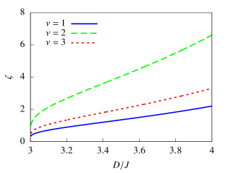
Figure 2: Plot of Eq. (11) with three solutions $\alpha_{1}=\frac{2}{9},\,\alpha_{2}=\frac{2}{3}$ ( both for ${\bm{K}}=0$), and $\alpha_{3}=\frac{1}{3}$ (for $\bm{K}=2\bm{Q}$). The cutoff scale is set at $\Lambda=2$.

Comparing the two solutions, we find that if we keep $J_{z}=\zeta J$ fixed and progressively reduce $D$ towards $3J$, the first instability occurs for the solution with $\alpha_{1}=\frac{2}{9}$. One can easily verify that the eigenfunction $B_{\bm{g}}^{(1)}$ for this solution is odd under spatial inversion ${\bm{g}}_{j}\to-{\bm{g}}_{j}$, i.e., viewed as a function of six elements of $g$, it behaves as

$$B_{\bm{g}}^{(1)}=(1,1,1,-1,-1,-1)^{\rm T}.$$ (12)

This in turn implies that that $\Psi_{{\bm{K}}=0}^{(1)}({\bm{q}})$ is an odd function of ${\bm{q}}$. Solving the actual equation on $B_{\bm{g}}^{(1)}$ by expanding $E({\bm{K}}=0)$ about its minimum and transforming from $B_{\bm{g}}$ to $\Psi_{\bm{K}}({\bm{p}})$ using the inverse of Eq. (6), we obtain

$$\Psi_{{\bm{K}}=0}^{(1)}({\bm{q}})=\frac{-2i\zeta J(\sin[q_{x}]-2\sin[\frac{q_{x}}{2}]\cos[\frac{\sqrt{3}q_{y}}{2}])}{4J(\cos[q_{x}]+2\cos[\frac{q_{x}}{2}]\cos[\frac{\sqrt{3}q_{y}}{2}])+6J+\epsilon_{b,1}}.$$ (13)

In real space, the corresponding $\psi^{(1)}_{n,m}=\psi({\bm{r}}={\bm{n}}-{\bm{m}})\sim\sin[{\bm{Q}}\cdot{\bm{r}}]e^{-r/\xi}$. The size of the exciton scales as $\xi\sim\epsilon_{b,1}^{-1/2}$.

For other c.m. momenta, a two-spin exciton also develops, but its energy becomes negative at a smaller $D<D_{1}$. Thus, for ${\bm{K}}=2{\bm{Q}}=2(4\pi/3,0)$, the minimum of the denominator in (9) occurs at ${\bm{q}}=0$. For small $\bm{q}$, the eigenvalue equation yields a single root $\alpha_{3}=\frac{1}{3}>\alpha_{1}$. This leads to the pair condensation at a smaller $D$ than for the parity-breaking solution $\alpha=\alpha_{1}$ (see Fig. 2).

As a hint what $E<0$ means, consider a finite density of bound pairs. Once the pairs condense, the new ground state at $D<D_{1}$ can be described at a mean-field level by the Jastrow wave function Zaletel et al. (2014):

$$|\Psi_{\rm CL}\rangle\sim e^{u\sum_{\bm{k}}\phi(\bm{k})S_{\bm{k}}^{+}S_{\bm{k}}^{-}}|0\rangle,$$ (14)

where the real function $\phi(\bm{k})=-\phi(-\bm{k})$ is odd under inversion, and $u$ is a real number. As a result, $\Psi_{\rm CL}$ breaks spatial inversion but preserves time-reversal symmetry. One can straightforwardly check that in this state the $z$ component of vector chirality ${\kappa}_{{\bm{n}}{\bm{m}}}$ is finite on every bond $\langle{\bm{n}},{\bm{m}}\rangle$ while $\langle{\bm{S}}_{\bm{n}}\rangle=0$ for every site ${\bm{n}}$. Therefore, (14) describes the CL state. The sign of $u$ selects the direction of the chiral order on a given bond and encodes $Z_{2}$ character of the CL phase. This state is also called a spin-current state Chubukov and Starykh (2013) because bond variables ${\kappa}_{{\bm{n}}{\bm{m}}}$ form oriented closed loops on every elementary triangle of the lattice.

III Schwinger boson formulation

III.1 SU(3) Schwinger boson representation

Having demonstrated the possibility of a VC order by analyzing the energy of a single two-spin exciton on top of the product $\otimes_{j}|S^{z}_{j}=0\rangle$ state, we now turn to the technical task of establishing its existence in the full many-body problem. For this, we need the formalism capable of treating both the large-$D$ paramagnetic state and the low-$D$ magnetically ordered state. Such a formulation is provided by the Schwinger boson theory Auerbach (1994) associated with the fundamental representation of SU(3) Muniz et al. (2014). The bosons obey the constraint, which needs to be fulfilled at every site ${\bm{r}}$ of the lattice,

$$\sum_{m}b^{\dagger}_{{\bm{r}}m}b^{\;}_{{\bm{r}}m}=1,$$ (15)

with $m=\{\uparrow,0,\downarrow\}$ label eigenvectors of $S^{z}_{\bm{r}}$: $S^{z}_{\bm{r}}b^{\dagger}_{{\bm{r}}m}|0\rangle=s^{z}_{m}b^{\dagger}_{{\bm{r}}m}|0\rangle$ with $s^{z}_{\uparrow}=1,s^{z}_{0}=0$, and $s^{z}_{\downarrow}=-1$. We will enforce the constraint in Eq. (15) by introducing the Lagrange multipliers $\mu_{\bm{r}}$:

$${\bar{\cal H}}={\cal H}+\sum_{\bm{r}}\mu_{\bm{r}}(b^{\dagger}_{{\bm{r}}\uparrow}b_{{\bm{r}}\uparrow}+b^{\dagger}_{{\bm{r}}\downarrow}b_{{\bm{r}}\downarrow}+b^{\dagger}_{{\bm{r}}0}b_{{\bm{r}}0}-1).$$ (16)

The spin operators $S^{\mu}_{\bm{r}}$ are bilinear forms of Schwinger bosons

$$S^{z}_{\bm{r}} ={\bm{b}}^{\dagger}_{{\bm{r}}}{\cal S}^{z}{\bm{b}}^{\;}_{{\bm{r}}}=b^{\dagger}_{{\bm{r}}\uparrow}b^{\;}_{{\bm{r}}\uparrow}-b^{\dagger}_{{\bm{r}}\downarrow}b^{\;}_{{\bm{r}}\downarrow},$$ (17a)

$$S^{+}_{\bm{r}} ={\bm{b}}^{\dagger}_{{\bm{r}}}{\cal S}^{+}{\bm{b}}^{\;}_{{\bm{r}}}=\sqrt{2}(b^{\dagger}_{{\bm{r}}\uparrow}b^{\;}_{{\bm{r}}0}+b^{\dagger}_{{\bm{r}}0}b^{\;}_{{\bm{r}}\downarrow}),$$ (17b)

$$S^{-}_{\bm{r}} ={\bm{b}}^{\dagger}_{{\bm{r}}}{\cal S}^{-}{\bm{b}}^{\;}_{{\bm{r}}}=\sqrt{2}(b^{\dagger}_{{\bm{r}}\downarrow}b^{\;}_{{\bm{r}}0}+b^{\dagger}_{{\bm{r}}0}b^{\;}_{{\bm{r}}\uparrow}),$$ (17c)

where we defined

$${\bm{b}}_{{\bm{r}}}=\left(\begin{array}[]{ccc}b_{{\bm{r}}\uparrow}&b_{{\bm{r}}0}&b_{{\bm{r}}\downarrow}\end{array}\right)^{T}.$$ (18)

With these expressions, we can write ${\cal H}$ as

$${\cal H}=\sum_{{\bm{r}},\nu,\mu}J_{\mu}{\bm{b}}^{\dagger}_{\bm{r}}{\cal S}^{\mu}{\bm{b}}^{\;}_{{\bm{r}}}{\bm{b}}^{\dagger}_{{\bm{r}}+{\bm{e}}_{\nu}}{\cal S}^{\mu}{\bm{b}}^{\;}_{{\bm{r}}+{\bm{e}}_{\nu}}+D\sum_{{\bm{r}}}(1-{\bm{b}}^{\dagger}_{\bm{r}}{\cal A}{\bm{b}}^{\;}_{{\bm{r}}}),$$

where ${\cal A}_{\alpha,\beta}=\delta_{\alpha,0}\delta_{\beta,0}$. The last term in this expression represents $(S^{z}_{{\bm{r}}})^{2}$ which reduces to $1-b^{\dagger}_{{\bm{r}}0}b^{\;}_{{\bm{r}}0}$ because of the constraint (15). The product state at large $D$ is recovered if we introduce the condensate of $b_{{\bm{r}}0}$ boson, i.e., replace $b_{{\bm{r}}0}$ and $b^{\dagger}_{{\bm{r}}0}$ operators by $b^{\dagger}_{{\bm{r}}0}=b^{\;}_{{\bm{r}}0}=s$ and set $s=1$. By continuity, $s$ remains nonzero in the whole paramagnetic state.

After condensing $b^{\dagger}_{{\bm{r}}0}$ in Eq. (17), spin operators $S^{\pm}_{\bm{r}}$ become proportional to $(b^{\dagger}_{{\bm{r}}\uparrow}+b^{\;}_{{\bm{r}}\downarrow})$ while $S^{z}_{\bm{r}}$ retains its quadratic form (17). The quadratic form of the spin-wave Hamiltonian (III.1) can now be written easily as

$${\bar{\cal H}}_{sw} = \sum_{{\bm{r}},\nu,\sigma}s^{2}J(b^{\dagger}_{{\bm{r}}\sigma}+b^{\;}_{{\bm{r}}{\bar{\sigma}}})(b^{\dagger}_{{\bm{r}}+{\bm{e}}_{\nu}{\bar{\sigma}}}+b^{\;}_{{\bm{r}}+{\bm{e}}_{\nu}\sigma})$$ (20)

$$+\mu\sum_{{\bm{r}},\sigma}n_{{\bm{r}}\sigma}+N(\mu-D)(s^{2}-1),$$

where $\sigma=\{\uparrow,\downarrow\}$, and $N$ is the total number of sites. The constraint is imposed on average, via the replacement $\mu_{\bm{r}}\to\mu$. By Fourier transforming the bosonic operators, ${b}^{\;}_{{\bm{k}}\sigma}=\frac{1}{\sqrt{N}}\sum_{\bm{r}}b^{\;}_{{\bm{r}}\sigma}e^{i{\bm{k}}\cdot{\bm{r}}}$, we obtain ${\bar{\cal H}}_{sw}$ in momentum space:

$${\bar{\cal H}}_{sw} = \sum_{{\bm{k}},\sigma}(\mu+s^{2}\epsilon_{\bm{k}}){b}^{\dagger}_{{\bm{k}}\sigma}{b}^{\;}_{{\bm{k}}{\sigma}}+N(\mu-D)(s^{2}-1)$$ (21)

$$+ \sum_{{\bm{k}},\sigma}\frac{s^{2}\epsilon_{\bm{k}}}{2}({b}^{\dagger}_{{\bm{k}}\sigma}{b}^{\dagger}_{-{\bm{k}}{\bar{\sigma}}}+\text{H.c.}),$$

with $\epsilon_{\bm{k}}=2J\gamma_{\bm{k}}$, $\gamma_{\bm{k}}=\sum_{\nu}\cos{{\bm{k}}\cdot{\bm{e}}_{\nu}}$. ${\bar{\cal H}}_{sw}$ is diagonalized by means of a Bogoliubov transformation:

$${b}^{\;}_{{\bm{k}}\sigma}=u_{\bm{k}}{\gamma}^{\;}_{{\bm{k}}\sigma}+v_{\bm{k}}{\gamma}^{\dagger}_{-{\bm{k}}{\bar{\sigma}}},$$ (22)

with

$$u_{\bm{k}} =(\mu+\omega_{\bm{k}})/\left(2\sqrt{\mu\omega_{\bm{k}}}\right),$$ (23a)

$$v_{\bm{k}} =(\mu-\omega_{\bm{k}})/\left(2\sqrt{\mu\omega_{\bm{k}}}\right),$$ (23b)

$$\omega_{\bm{k}} =\sqrt{\mu^{2}+2\mu s^{2}\epsilon_{\bm{k}}}.$$ (23c)

The diagonal form of ${\bar{\cal H}}_{sw}$ is:

$${\bar{\cal H}}_{sw}\!=\!N(\mu-D)(s^{2}-1)\!+\!\sum_{{\bm{k}}\sigma}\!\left[\omega_{\bm{k}}(\gamma^{\dagger}_{{\bm{k}}\sigma}\gamma^{\;}_{{\bm{k}}\sigma}+\frac{1}{2})-\frac{\mu}{2}\right]\!.$$ (24)

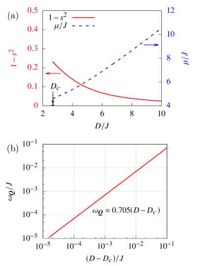
Figure 3: (a) Dependence of saddle-point parameters $s$ and $\mu$ on $D/J$ [as indicated in Eq. (26), there is no $\zeta$ dependence]. $D_{c}/J\approx 2.68$ indicates the quantum critical point of single-magnon condensation below which long-range magnetic order develops. (b) Magnitude of the single-magnon gap $\omega_{\bm{Q}}$ near the critical point $D-D_{c}\ll J$.

The dispersion relation $\omega_{\bm{k}}$ has minima at the wave vectors $\pm{\bm{Q}}=\pm(4\pi/3,0)$, and the paramagnetic state remains stable against spin-wave excitations as long as $\omega^{2}_{\bm{Q}}>0$. The variational parameters $s$ and $\mu$ are obtained from the saddle-point equations, $\partial E_{0}^{\text{PM}}/\partial s=0$ and $\partial E_{0}^{\text{PM}}/\partial\mu=0$, where $E_{0}^{\text{PM}}$ is the ground-state energy density:

$$E_{0}^{\text{PM}}=\frac{1}{N}\sum_{\bm{k}}\omega_{\bm{k}}+(\mu-D)(s^{2}-1)-\mu.$$ (25)

The resulting self-consistent equations are:

$$s^{2} =2-\int\frac{d\bm{k}}{V_{\text{BZ}}}\frac{\mu+s^{2}\epsilon_{\bm{k}}}{\omega_{\bm{k}}},$$ (26a)

$$D =\mu\left(1+\int\frac{d\bm{k}}{V_{\text{BZ}}}\frac{\epsilon_{\bm{k}}}{\omega_{\bm{k}}}\right),$$ (26b)

where $V_{\text{BZ}}=\frac{8\pi^{2}}{\sqrt{3}}$ is the size of the first Brillouin zone.

The single-magnon gap $\omega_{\bm{Q}}$ vanishes at the phase boundary between the paramagnetic and the magnetically ordered phases. Combining this condition with Eq. (26) we obtain the critical value $D_{c}\approx 2.68J$ [see Fig. 3]. The downward renormalization of $D_{c}$ from its naive single-particle value of $3J$ to $D_{c}\approx 2.68J$ is caused by the renormalization of the large-$D$ paramagnetic ground state by quantum fluctuations, which are captured by our mean-field parameters $s$ and $\mu$. Note that the value of $D_{c}$, obtained this way, is in much better agreement with numerical results Zhang et al. (2013), than $D_{c}=6J$, obtained using more traditional Holstein-Primakoff–type approach Holstein and Primakoff (1940) (see Appendix B).

III.2 Interaction between modes

To analyze two-magnon bound states in a many-body system, we have to know the interaction between magnons. It comes from the Ising part of the Heisenberg interaction:

$${\cal H}^{(4)}_{\rm I}=\zeta J\sum_{{\bm{r}},\nu}(n_{{\bm{r}}\uparrow}-n_{{\bm{r}}{\downarrow}})(n_{{\bm{r}}+{\bm{e}}_{\nu}{\uparrow}}-n_{{\bm{r}}+{\bm{e}}_{\nu}\downarrow}).$$ (27)

The signs of separate terms in (27) show that the interaction is repulsive between magnons of the same spin and attractive between magnons with opposite spins. In momentum space

$${\cal H}^{(4)}_{\rm I}\!=\!\frac{1}{N}\!\!\sum_{{\bm{k}}_{1},{\bm{k}}_{2},{\bm{q}},\sigma,\sigma^{\prime}}\!\!\!\!V_{\sigma\sigma^{\prime}}({\bm{q}})b^{\dagger}_{\bm{k}_{1}+\bm{q}\sigma}b^{\dagger}_{\bm{k}_{2}-\bm{q}\sigma^{\prime}}b_{\bm{k}_{2}\sigma^{\prime}}b_{\bm{k}_{1}\sigma},$$ (28)

with $V_{\sigma\sigma^{\prime}}({\bm{q}})=\sigma\sigma^{\prime}\zeta J\gamma_{\bm{q}}.$

We will show below that an attractive interaction between the $\uparrow$ and $\downarrow$ magnons induces a two-particle bound state with $S_{z}=0$ in the full many-body system. The energy $E$ of this bound state vanishes at a critical value of $D=D^{b}_{c}>D_{c}$ above the single-magnon condensation transition, like in the earlier analysis of a single exciton. A vanishing gap of a two-magnon bound state signals a divergence of the susceptibility of an order parameter which is bilinear in spin operators. Based on our previous discussion, the obvious candidate is vector chirality. Condition $D^{b}_{c}>D_{c}$ means that the chiral susceptibility diverges while the ordinary magnetic susceptibility is still finite. This implies the quantum paramagnetic state and the magnetically ordered state are separated by the intermediate CL state. Crucial for this consideration is the fact that the single-magnon spectrum is two-fold degenerate, with minima at $\pm{\bm{Q}}$. This gives two choices for the sign of vector chirality and in CL state the system chooses one particular sign, spontaneously breaking $Z_{2}$ chiral symmetry.

To see this, we expand ${\cal H}^{(4)}_{\rm I}$ in terms of the Bogoliubov quasi-particle operators (22) as

$${\cal H}^{(4)}_{\rm I} =\frac{1}{N}\!\!\sum_{\bm{k}_{1},\bm{k}_{2},\bm{q}}\!\!V_{\bm{q}}^{22o}(\bm{k}_{1},\bm{k}_{2})\gamma_{\bm{k}_{1}+\bm{q}\uparrow}^{\dagger}\gamma_{\bm{k}_{2}-\bm{q}\downarrow}^{\dagger}\gamma_{\bm{k}_{2}\downarrow}\gamma_{\bm{k}_{1}\uparrow}$$

$$+\frac{1}{N}\!\!\sum_{\bm{k}_{1},\bm{k}_{2},\bm{q},\sigma}\!\!V_{\bm{q}}^{22s}(\bm{k}_{1},\bm{k}_{2})\gamma_{\bm{k}_{1}+\bm{q}\sigma}^{\dagger}\gamma_{\bm{k}_{2}-\bm{q}\sigma}^{\dagger}\gamma_{\bm{k}_{2}\sigma}\gamma_{\bm{k}_{1}\sigma}$$

$$+\frac{1}{N}\!\!\sum_{\bm{k}_{1},\bm{k}_{2},\bm{q},\sigma}\!\!\Big{[}V_{\bm{q}}^{31}(\bm{k}_{1},\bm{k}_{2})\gamma_{\bm{k}_{1}+\bm{q}\sigma}^{\dagger}\gamma_{\bm{k}_{1}\sigma}\gamma_{\bm{k}_{2}\sigma}\gamma_{-\bm{k}_{2}+\bm{q}\bar{\sigma}}$$

$$+V_{\bm{q}}^{40}(\bm{k}_{1},\bm{k}_{2})\gamma_{-\bm{k}_{1}-\bm{q}\uparrow}\gamma_{-\bm{k}_{2}+\bm{q}\downarrow}\gamma_{\bm{k}_{2}\downarrow}\gamma_{\bm{k}_{1}\uparrow}+\text{H.c.}\Big{]}.$$ (29)

The interaction vertices between spin-up and -down particles are given by

$$V_{\bm{q}}^{22o}({\bm{k}}_{1},{\bm{k}}_{2}) =2\Big{[}V_{\uparrow\uparrow}({\bm{k}_{1}+\bm{k}_{2}})B_{{\bm{k}}_{1},{\bm{k}}_{2}}B_{{\bm{k}_{1}+\bm{q}},{\bm{k}_{2}-\bm{q}}}$$

$$\quad+V_{\uparrow\downarrow}({\bm{q}})A_{{\bm{k}}_{1},\bm{k}_{1}+{\bm{q}}}A_{{\bm{k}}_{2},\bm{k}_{2}-{\bm{q}}}\Big{]},$$ (30a)

$$V_{\bm{q}}^{22s}({\bm{k}}_{1},{\bm{k}}_{2}) =\frac{V_{\uparrow\uparrow}({\bm{k}}_{1}-{\bm{k}}_{2}+{\bm{q}})}{2}A_{\bm{k}_{2},\bm{k}_{1}+\bm{q}}A_{\bm{k}_{1},\bm{k}_{2}-\bm{q}}$$

$$\quad+\frac{V_{\uparrow\uparrow}({\bm{q}})}{2}A_{{\bm{k}}_{1},\bm{k}_{1}+{\bm{q}}}A_{{\bm{k}}_{2},\bm{k}_{2}-{\bm{q}}},$$ (30b)

$$V_{\bm{q}}^{31}({\bm{k}}_{1},{\bm{k}}_{2}) =V_{\uparrow\uparrow}(\bm{k}_{1}-\bm{k}_{2}+\bm{q})A_{\bm{k}_{2},\bm{k}_{1}+\bm{q}}B_{\bm{k}_{1},\bm{k}_{2}-\bm{q}}$$

$$\quad+V_{\uparrow\uparrow}(\bm{q})A_{\bm{k}_{1},\bm{k}_{1}+\bm{q}}B_{\bm{k}_{2},\bm{k}_{2}-\bm{q}},$$ (30c)

$$V_{\bm{q}}^{40}({\bm{k}}_{1},{\bm{k}}_{2}) =-\frac{V_{\uparrow\uparrow}(\bm{k}_{1}-\bm{k}_{2}+\bm{q})}{2}B_{\bm{k}_{1},\bm{k}_{2}-\bm{q}}B_{\bm{k}_{2},\bm{k}_{1}+\bm{q}}$$

$$\quad+\frac{V_{\uparrow\uparrow}(\bm{k}_{1}+\bm{k}_{2})}{2}B_{\bm{k}_{1},\bm{k}_{2}}B_{\bm{k}_{1}+\bm{q},\bm{k}_{2}-\bm{q}},$$ (30d)

where

$$A_{{\bm{k}}_{1},{\bm{k}}_{2}} \equiv u_{{\bm{k}}_{1}}u_{{\bm{k}}_{2}}-v_{{\bm{k}}_{1}}v_{{\bm{k}}_{2}}=\frac{\omega_{\bm{k}_{1}}+\omega_{\bm{k}_{2}}}{2\sqrt{\omega_{\bm{k}_{1}}\omega_{\bm{k}_{2}}}},$$ (31a)

$$B_{{\bm{k}}_{1},{\bm{k}}_{2}} \equiv u_{{\bm{k}}_{1}}v_{{\bm{k}}_{2}}-v_{{\bm{k}}_{1}}u_{{\bm{k}}_{2}}=\frac{\omega_{\bm{k}_{1}}-\omega_{\bm{k}_{2}}}{2\sqrt{\omega_{\bm{k}_{1}}\omega_{\bm{k}_{2}}}}.$$ (31b)

And, we remind, $V_{\sigma\sigma^{\prime}}({\bm{q}})=\sigma\sigma^{\prime}\zeta J\gamma_{\bm{q}}$.

III.3 Order Parameter and its Equation of Motion

It is useful to develop some intuition before addressing the issue of bound-state condensation in the many-body problem represented by the Hamiltonian (III.2). In the analysis in Sec. II.2 we selected staggered vector chirality as the candidate for the two-magnon order parameter. (Neighboring up- and down-pointing triangles have opposite chirality.) This order parameter is expressed as

$$\kappa=\frac{1}{N}\sum_{{\bm{r}}\in\triangledown}\hat{z}\cdot\sum_{j=1}^{3}\langle{\bm{S}}_{\bm{r}}\times{\bm{S}}_{{\bm{r}}+{\bm{e}}_{j}}\rangle,$$ (32)

where the sum is over down-pointing triangles of the lattice and we go clockwise within a triangle. The brackets denote average over the ground state. In momentum space the vector chirality reads

$$\kappa=-\frac{1}{N}\sum_{\bm{q}}\sum_{j=1}^{3}\sin[{\bm{q}}\cdot{\bm{e}}_{j}]\langle S^{+}_{\bm{q}}S^{-}_{-{\bm{q}}}\rangle.$$ (33)

In terms of Bogoliubov eigenmodes, this becomes

$$\kappa = -\frac{2s^{2}}{N}\sum_{\bm{q}}\sum_{j=1}^{3}\sin[{\bm{q}}\cdot{\bm{e}}_{j}](u_{\bm{q}}+v_{\bm{q}})^{2}$$ (34)

$$\times\langle(\gamma^{\dagger}_{-{\bm{q}}\uparrow}+\gamma_{{\bm{q}}\downarrow})(\gamma_{-{\bm{q}}\uparrow}+\gamma^{\dagger}_{{\bm{q}}\downarrow})\rangle.$$

In the low-energy long-wavelength approximation we focus on the lowest-energy magnons with ${\bm{q}}=\pm{\bm{Q}}$. In terms of these magnons, vector chirality is expressed as

$$\kappa=-\frac{3\sqrt{3}\mu s^{2}}{N\omega_{\bm{Q}}}\langle\gamma^{\dagger}_{-{\bm{Q}}\uparrow}\gamma^{\dagger}_{{\bm{Q}}\downarrow}-\gamma^{\dagger}_{{\bm{Q}}\uparrow}\gamma^{\dagger}_{-{\bm{Q}}\downarrow}+{\text{H.c.}}\rangle.$$ (35)

This result shows that vector chirality is associated with the appearance of the bound state in the antisymmetric $S^{z}=0$ channel: $\kappa$ changes sign under ${\bm{Q}}\to-{\bm{Q}}$ and is formed by $\uparrow$ and $\downarrow$ magnons. We then introduce, by analogy with superconductivity, composite pair operators

$$\phi_{L}(\bm{k}) \equiv\gamma_{\bm{Q}-\bm{k}\uparrow}\gamma_{\bar{\bm{Q}}+\bm{k}\downarrow},$$ (36a)

$$\phi_{R}(\bm{k}) \equiv\gamma_{\bar{\bm{Q}}+\bm{k}\uparrow}\gamma_{\bm{Q}-\bm{k}\downarrow}.$$ (36b)

where here and below we label ${\bar{\bm{Q}}}\equiv-{\bm{Q}}$. The long-wavelength limit corresponds to small ${\bm{k}}$. The vector chirality is related to average values of these pair operators

$$\kappa=-\frac{3\sqrt{3}\mu s^{2}}{N\omega_{\bm{Q}}}\left(\phi^{*}_{R}+\phi_{R}-\phi^{*}_{L}-\phi_{L}\right).$$ (37)

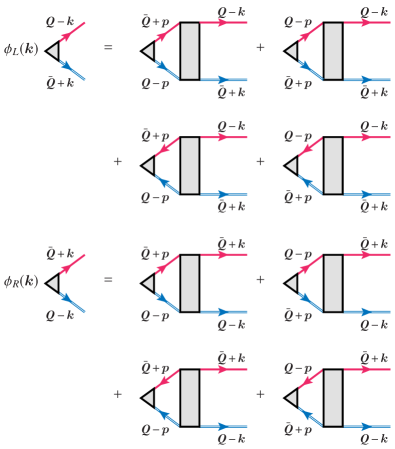
Figure 4: Equations for the vertices $\phi_{L/R}(\bm{k})$. The shaded rectangles denote the fully dressed irreducible interactions between low-energy magnons. Solid (red) and hollow (blue) oriented lines represent spin $\uparrow$ and $\downarrow$ magnons, correspondingly.

The equations for $\phi_{R/L}({\bm{k}})$ are presented graphically in Fig. 4. The shaded vertices in this figure are fully dressed irreducible interactions in the particle-particle channel (internal magnons have opposite frequencies $\pm\epsilon$ and momenta ${\bm{Q}}-{\bm{p}}$ and ${\bar{\bm{Q}}}+{\bm{p}}$). We verified that the particle number non-conserving dressed vertex $V_{\bm{q}}^{31}$ as well as the dressed vertex $V_{\bm{q}}^{22s}$, which is symmetric in the spin index $\sigma$, do not directly contribute to the renormalizations of $\phi_{R/L}$. We also verified that magnon self-energy does not affect the formation of two-magnon bound state in any qualitative way and is therefore irrelevant for our purposes. Finally, the set of equations for $\phi_{R}$ and $\phi_{L}$ can be re-arranged as the subset for $\phi_{R}-\phi_{L}$ and the one for $\phi_{R}+\phi_{L}$. We find that the pairing interaction is stronger for $\phi_{R}-\phi_{L}$, in agreement with vector-chiral nature (35) of the anticipated order, and focus on it below (see Chubukov and Starykh (2013) for similar manipulations). Collecting the diagrams in Fig. 4, we obtain an integral equation

$$\frac{1}{N}\!\!\sum_{\bm{p}}\frac{F_{\bm{k},\bm{p}}^{22o}\,\theta_{\bm{p}}-4F_{\bm{k},\bm{p}}^{04}\,\theta_{\bm{p}}^{*}}{2\omega_{\bm{Q}-\bm{p}}}=-\theta_{\bm{k}}.$$ (38)

Here, $\theta_{\bm{k}}\equiv 2\omega_{{\bm{Q}}-{\bm{k}}}\langle\phi_{R}(\bm{k})-\phi_{L}(\bm{k})\rangle$ and

$$F_{\bm{k},\bm{p}}^{22o} \equiv\Gamma_{\bm{k}-\bm{p}}^{22o}(\bar{\bm{Q}}\!+\!\bm{p},\bm{Q}\!-\!\bm{p})-\Gamma_{2\bm{Q}-\bm{p}-\bm{k}}^{22o}(\bar{\bm{Q}}\!+\!\bm{p},\bm{Q}\!-\!\bm{p}),$$ (39a)

$$F_{\bm{k},\bm{p}}^{04} \equiv\Gamma_{\bm{k}-\bm{p}}^{04}(\bar{\bm{Q}}\!+\!\bm{p},\bm{Q}\!-\!\bm{p})\!-\!\Gamma_{2\bm{Q}-\bm{p}-\bm{k}}^{04}(\bar{\bm{Q}}\!+\!\bm{p},\bm{Q}\!-\!\bm{p}),$$ (39b)

where $\Gamma$’s are the fully dressed irreducible vertices between magnons with opposite frequencies. Each $\Gamma$ term originates from the corresponding interaction term in the Hamiltonian, e.g., $\Gamma_{\bm{k}-\bm{p}}^{22o}(\bar{\bm{Q}}\!+\!\bm{p},\bm{Q}\!-\!\bm{p})$ originates from $V_{\bm{k}-\bm{p}}^{22o}(\bar{\bm{Q}}\!+\!\bm{p},\bm{Q}\!-\!\bm{p})$. The factor $1/(2\omega_{\bm{Q}-\bm{p}})$ comes from the integration over the frequency of internal magnon lines, e.g.

$$\int\frac{d\epsilon}{2\pi}\frac{1}{\epsilon-\omega_{\bm{Q}-\bm{p}}+i\delta}\frac{1}{-\epsilon-\omega_{-\bm{Q}+\bm{p}}+i\delta}=\frac{i}{2\omega_{\bm{Q}-\bm{p}}}.$$ (40)

The equation identical to (38) can be also obtained from the equation of motion for the chiral combination $\theta_{\bm{k}}$, see Chubukov and Starykh (2013). The appearance of a nontrivial solution of Eq. (38) signals the instability of many-body paramagnetic ground state towards the condensation of two-magnon bound pairs.

Equation (38) highlights the role of the particle number non-conserving terms $\Gamma_{\bm{q}}^{40}$ and $\Gamma_{\bm{q}}^{04}$ [second line of (38)]. Without them, the equation for $\theta_{\bm{k}}$ is U(1) degenerate: a solution $\theta_{0}$ is defined up to a complex phase, i.e., there is a degeneracy in the order-parameter manifold. Such degeneracy is lifted by the anomalous terms, which depend on $\theta^{*}_{\bm{p}}$. The solutions with real and imaginary $\theta_{\bm{p}}$ now become different and the system chooses one of them. One can easily verify that the state with VC order parameter $\kappa\neq 0$ develops if the solution $\theta_{p}$ is real. The real solution preserves time-reversal symmetry, as expected for the VC order. On the contrary, if the solution of (38) is imaginary, it yields an order parameter that breaks time-reversal symmetry rather than vector chirality.

III.4 Solution for the bound state at small $J_{z}$

We now analyze the structure of the interactions in (38) in the perturbative limit of small $J_{z}$. Because each interaction term in the Hamiltonian has $J_{z}$ as the overall factor, a non-zero solution for $\theta_{p}$ emerges only if the overall smallness of the interaction is compensated by the singularity of the momentum integral in the kernel, much like it happens in BCS theory of superconductivity. We argue below that the same happens in our case, but the singularity emerges at order $J^{2}_{z}$, once we include the renormalizations of the interaction vertices. In this respect, the pairing that we find is similar to Kohn-Luttinger effect in the theory of superconductivity Kohn and Luttinger (1965).

III.4.1 First order in $J_{z}$

To first order in $J_{z}$, the vertices $\Gamma$ in Eq. (38) coincide with the interaction terms $V$ in the Hamiltonian. There is a potential for singular behavior of the kernel as it contains $1/\omega_{\bm{Q}-\bm{p}}$ which becomes singular at $\bm{p}=0$ and at $D=D_{c}$, where single-magnon excitations condense. One can easily check that at small ${\bm{p}}$ and small ${\bm{k}}$, the prefactors for $\theta_{\bm{p}}$ and $\theta_{\bm{p}}^{*}$ in  (38) are negative. This implies that (i) the pairing interaction is attractive, and (ii) the strongest attraction is for real $\theta_{{\bm{k}}}$. Using the explicit forms of the bare interactions [Eq. (30)], we find that at small ${\bm{k}}$ and ${\bm{p}}$ all four interactions $V$ in Eq.  (38) are of order one in units of $J_{z}$, because $A_{\bm{k}_{1},\bm{k}_{2}}$ and $B_{\bm{k}_{1},\bm{k}_{2}}$ in (31) are $O(1)$:

$$F_{\bm{k},\bm{p}}^{22o}=-4F_{\bm{k},\bm{p}}^{04}\approx-\frac{9}{4}J_{z}\frac{(\omega_{\bm{Q}-\bm{p}}+\omega_{\bm{Q}-\bm{k}})^{2}}{\omega_{\bm{Q}-\bm{p}}\omega_{\bm{Q}-\bm{k}}}.$$ (41)

In this situation, $\theta_{\bm{k}}$ depends on ${\bm{k}}$ in a non-singular way, and the condition that $\theta_{\bm{k}}$ is non-zero reduces to

$$1=a\frac{J_{z}}{N}\sum_{\bm{p}}\frac{1}{\omega_{\bm{Q}-\bm{p}}}.$$ (42)

where $a=O(1)$ is a numerical coefficient. Since $\omega_{\bm{Q}}$ vanishes at $D=D_{c}$, the kernel is singular. However, the singularity is integrable because $\omega_{\bm{Q}-\bm{p}}$ scales linearly in $|{\bm{p}}|$ at $D=D_{c}$. This implies that there is no instability towards CL state at small $J_{z}$, as long as we use bare interactions in Eq. (38).

The reason for the absence of the instability is related to specific property of $A_{\bm{k}_{1},\bm{k}_{2}}$ and $B_{\bm{k}_{1},\bm{k}_{2}}$ which determine the interaction terms $V$ in the Hamiltonian. Namely, when $\bm{k}_{1}$ and $\bm{k}_{2}$ are close to $\pm{\bm{Q}}$, $A_{\bm{k}_{1},\bm{k}_{2}}$ and $B_{\bm{k}_{1},\bm{k}_{2}}$ are $O(1)$. This is what we used in the derivation of Eq. (42). On the other hand, if only one wave vector, say ${\bm{k}}_{1}$, is near $\pm{\bm{Q}}$, i.e., $\omega_{{\bm{k}}_{1}}$ is small, while the other one, ${\bm{k}}_{2}$, is sufficiently far from $\pm{\bm{Q}}$ so that $\omega_{{\bm{k}}_{2}}=O(J)$, both $A_{\bm{k}_{1},\bm{k}_{2}}$ and $B_{\bm{k}_{1},\bm{k}_{2}}$ scale as $\sqrt{\omega_{\bm{k}_{2}}/\omega_{\bm{k}_{1}}}\gg 1$. This implies that the interactions $V_{\bm{q}}^{22o}(\bm{k}_{1},\bm{k}_{2})$ and $V_{\bm{q}}^{40}(\bm{k}_{1},\bm{k}_{2})$ are $\sim O(1)$ only when all incoming/outgoing momenta are small, but become much larger when one momentum remains near $\pm\bm{Q}$, while another one moves away from $\pm\bm{Q}$.

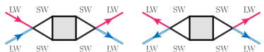
Figure 5: Schematics of the processes which contribute to relevant renormalization of the interactions $V_{\bm{q}}^{22o}$ (left) and $V_{\bm{q}}^{04}$ (right) between low-wavelength (LW) magnons by short-wavelength (SW) magnons with momenta far away from $\pm\bm{Q}$. Complete list of diagrams to second order in $J_{z}$ is in Figs. 6 and 7. The renormalized interactions $\Gamma$ scale as $O(J^{2}_{z}/\omega_{\bm{Q}}^{2})$ and are much stronger than bare interactions $V\sim J_{z}$.

This observation suggests that one can potentially get a much stronger dressed interaction between low-energy bosons, if one includes the renormalization of interaction vertices $V^{\cdots}_{\bm{q}}(\bm{k}_{1},\bm{k}_{2})$ by virtual processes involving bosons with momenta far away from ${\pm\bm{Q}}$ (see Fig. 5 for schematic illustration). To verify this, we now compute the dressed vertices $\Gamma$ to order $J^{2}_{z}$.

III.4.2 Second order in $J_{z}$

The irreducible interactions $\Gamma$ to order $J^{2}_{z}$ come from three sets of processes: the $2\rightarrow 2$ processes that conserves number of bosons, and $0\rightarrow 4$ ($4\rightarrow 0$) and $1\rightarrow 3$ ($3\rightarrow 1$) processes that create or annihilate additional bosons. The external momenta in the vertices are fixed at $p,\,k\ll Q$, while the internal ones are not assumed to be small, and are integrated over the first Brillouin zone.

The relevant second order diagrams for $\Gamma_{\bm{k}-\bm{p}}^{22o}(\bar{\bm{Q}}+\bm{p},\bm{Q}-\bm{p})$ are shown in Fig. 6. The diagrams for $\Gamma_{2\bm{Q}-\bm{k}-\bm{p}}^{22o}(\bar{\bm{Q}}+\bm{p},\bm{Q}-\bm{p})$ are the same except for different momentum labels. Summing up contributions from all six diagrams, we obtain

$$F_{\bm{k},\bm{p}}^{22o}=-\frac{\zeta^{2}s^{2}J^{3}}{8\omega_{\bm{Q}-\bm{p}}\omega_{\bm{Q}-\bm{k}}}\sum_{i=1}^{6}\beta_{i},$$ (43)

where $\beta_{i}$ are numerical factors listed in Fig. 6.

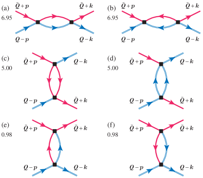
Figure 6: Nonzero second-order diagrams for the effective vertices $\Gamma_{\bm{k}-\bm{p}}^{22o}(\bar{\bm{Q}}+\bm{p},\bm{Q}-\bm{p})$. The diagrams for $\Gamma_{2\bm{Q}-\bm{k}-\bm{p}}^{22o}(\bar{\bm{Q}}+\bm{p},\bm{Q}-\bm{p})$ are the same, except for different momentum labels. Solid (red) and hollow (blue) oriented lines represent Green’s function of spin $\uparrow$ and $\downarrow$ magnons, correspondingly. The value of $\beta_{i}$ in Eq. (43) is listed separately for each diagram.

Similarly, the second-order renormalization of the anomalous vertices (see Fig. 7) yields

$$-4F_{\bm{k},\bm{p}}^{04}=-\frac{\zeta^{2}s^{2}J^{3}}{8\omega_{\bm{Q}-\bm{p}}\omega_{\bm{Q}-\bm{k}}}\sum_{i=1}^{6}{\bar{\beta}}_{i},$$ (44)

where ${\bar{\beta}_{i}}$ are numerical factors listed in Fig. 7.

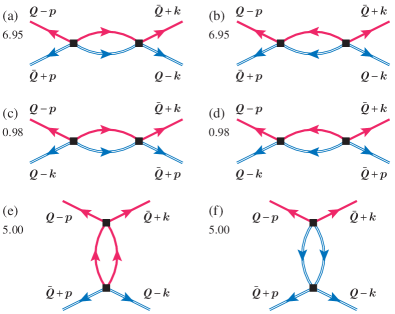
Figure 7: Nonzero second-order diagrams for the effective vertices $\Gamma_{\bm{k}-\bm{p}}^{04}(\bar{\bm{Q}}+\bm{p},\bm{Q}-\bm{p})$. The diagrams for $\Gamma_{2\bm{Q}-\bm{k}-\bm{p}}^{04}(\bar{\bm{Q}}+\bm{p},\bm{Q}-\bm{p})$ are the same, except for different momentum labels. Solid (red) and hollow (blue) oriented lines represent Green’s function of spin $\uparrow$ and $\downarrow$ magnons, correspondingly. The value of ${\bar{\beta}}_{i}$ in Eq. (44) is listed separately for each diagram.

We see that

$$\quad F_{\bm{k},\bm{p}}^{22o}=-4F_{\bm{k},\bm{p}}^{04}$$

$$=-\frac{25.86s^{2}}{8}~{}\frac{\zeta^{2}J^{3}}{\omega_{\bm{Q}-\bm{p}}\omega_{\bm{Q}-\bm{k}}}\approx-2.49\frac{\zeta^{2}J^{3}}{\omega_{\bm{Q}-\bm{p}}\omega_{\bm{Q}-\bm{k}}},$$ (45)

where we used $s^{2}=0.77$ (at $D=D_{c}$) for the condensate of the $b_{\bm{r}0}$ boson $s=\langle b_{{\bm{r}}0}\rangle$ (see Fig. 3). We emphasize that (i) the dressed interaction is negative, i.e., attractive, (ii) the interplay between normal and anomalous vertices remains exactly the same as for bare interaction, i.e., the largest attraction is for the real order parameter $\theta_{{\bm{k}}}$, and (iii) the attractive interaction now scales as $1/(\omega_{\bm{Q}-\bm{p}}\omega_{\bm{Q}-\bm{k}})$, i.e., the pairing vertex becomes truly singular at small $k$ and $p$.

Substituting Eq. (45) into (38) we obtain integral equation on $\theta_{{\bm{k}}}$, with $\alpha=3.23s^{2}=2.49$:

$$\frac{1}{N}\sum_{\bm{p}}\frac{\alpha\zeta^{2}J^{3}}{\omega_{\bm{Q}-\bm{p}}^{2}\omega_{\bm{Q}-\bm{k}}}\theta_{\bm{p}}=\theta_{\bm{k}}.$$ (46)

Equation (46) shows that the combination ${\cal C}=\omega_{\bm{Q}-\bm{k}}\theta_{\bm{k}}$ is actually ${\bm{k}}$ independent. This allows one to transform it into the self-consistent equation which reads as

$$\frac{1}{\alpha\zeta^{2}J^{3}}=\frac{1}{N}\sum_{\bm{p}}\frac{1}{\omega^{3}_{\bm{Q}-\bm{p}}}\approx\frac{1}{N}\sum_{\bm{p}}\frac{1}{(\omega_{\bm{Q}}^{2}+9J^{2}s^{4}p^{2})^{3/2}}.$$ (47)

The integral in the right-hand side is easily evaluated to be $1/(18\pi J^{2}s^{4}\omega_{\bm{Q}})$. Importantly, it scales as $1/\omega_{\bm{Q}}$ and therefore diverges as $D\to D_{c}$. Using $\omega_{\bm{Q}}\approx 0.705(D-D_{c})$ (see Figure 3), we obtain the critical value $D^{b}_{c}$ for the instability towards CL state:

$$D^{b}_{c}=D_{c}+0.042\alpha\zeta^{2}J$$ (48)

We see that $D^{c}_{b}>D_{c}$ for arbitrary small $\zeta=J_{z}/J$, hence, there is no threshold on the strength of the interaction for the emergence of CL phase.

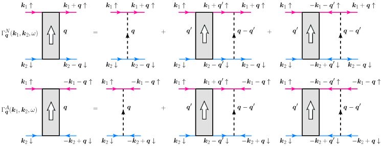
Figure 8: The diagrammatic representation of the Bethe-Salpeter equation.

Before we move to the analysis at arbitrary $J_{z}$, a comment is in order. Within the saddle-point approximation of Eq. (26), $\omega_{\bm{Q}}\propto(D-D_{c})$ [we used this relation above to obtain (48)]. This approximation becomes exact in the limit $N\to\infty$, where $N$ is the number of bosonic flavors Zhang et al. (2013). In contrast, the more traditional Holstein-Primakoff mean-field approach leads to $\omega_{\bm{Q}}\propto(D-D_{c})^{1/2}$ (see Appendix). None of these exponents is actually the exact one because the dimension of the effective theory in our case, $D_{\rm dim}=d+1=3$, is lower than the upper critical dimension $D_{\rm dim}=4$. Moreover, a perturbative ($\epsilon$-expansion) renormalization group analysis shows that there is no stable fixed point for the simultaneous breaking of the continuous U(1) and the discrete $Z_{2}$ symmetries Kamiya et al. (2011); Parker and Balents (2017), i.e., at $J_{z}=0$ the transition at $D_{c}$ would be weakly first order. If we take this into account, we find that the intermediate CL phase still emerges, but for $J_{z}$ above some small but finite value. This is because $\omega_{\bm{Q}}$ remains finite at a first-order transition, and a finite $J_{z}$ is needed for the bound state to form.

III.5 Bethe-Salpeter equation

In the previous section, we obtained the instability of a paramagnet towards a CL state at small $J_{z}$ by analyzing the equations on the pair fields $\phi_{L}(\bm{k})$ and $\phi_{R}(\bm{k})$. In this section, we use a complementary approach and extract the information about two-particle bound states from the poles of the four-point vertex function. This last approach can be rigorously justified in the opposite limit when $J_{z}$ is large enough such that the instability towards CL state occurs while the density of bosons is still small. The bosonic density is $\langle b^{\dagger}_{{\bm{k}}\sigma}b_{{\bm{k}}\sigma}\rangle=v_{\bm{k}}^{2}$, where, we remind, $v_{\bm{k}}$ is the Bogoliubov parameter, defined in Eqs. (22) and (23). Below we assume that $v_{\bm{k}}$ is small at $D=D^{b}_{c}$ and keep only the leading-order terms in $v_{\bm{k}}$. In our notations, $v_{\bm{k}}$ is small when the Lagrange multiplier $\mu$ is large [see Eq. (23)]. Figure 3 shows that $\mu$ is large in a wide range of $D>D_{c}$.

The fully renormalized normal and anomalous four-point vertex functions $\Gamma_{\bm{q}}^{N}(\bm{k}_{1},\bm{k}_{2},\omega)$ and $\Gamma_{\bm{q}}^{A}(\bm{k}_{1},\bm{k}_{2},\omega)$, with incoming frequency $\omega$, are obtained by solving the Bethe-Salpeter (BS) equations. Within our approximation, these equations reduce to the ones shown in Fig. 8. In analytic form

$$\quad\Gamma_{\bm{q}}^{N}(\bm{k}_{1},\bm{k}_{2},\omega)-V_{\bm{q}}^{22o}(\bm{k}_{1},\bm{k}_{2})$$

$$=-\int\frac{d{\bm{q}}^{\prime}}{V_{\text{BZ}}}\frac{\Gamma_{\bm{q}^{\prime}}^{N}(\bm{k}_{1},\bm{k}_{2},\omega)V_{{\bm{q}}-{\bm{q}^{\prime}}}^{22o}({\bm{k}}_{1}+{\bm{q}}^{\prime},{\bm{k}}_{2}-{\bm{q}}^{\prime})}{\omega_{{\bm{k}}_{1}+{\bm{q}}^{\prime}}+\omega_{{\bm{k}}_{2}-{\bm{q}}^{\prime}}-\omega}$$

$$-\int\frac{d\bm{q}^{\prime}}{V_{\text{BZ}}}\frac{16\Gamma_{\bm{q}^{\prime}}^{A}(\bm{k}_{1},\bm{k}_{2},\omega)V_{\bm{q}-\bm{q}^{\prime}}^{04}(\bm{k}_{1}+\bm{q}^{\prime},\bm{k}_{2}-\bm{q}^{\prime})}{\omega_{\bm{k}_{1}+\bm{q}^{\prime}}+\omega_{\bm{k}_{2}-\bm{q}^{\prime}}+\omega},$$ (49a)

$$\quad\Gamma_{\bm{q}}^{A}(\bm{k}_{1},\bm{k}_{2},\omega)-V_{\bm{q}}^{40}(\bm{k}_{1},\bm{k}_{2})$$

$$=-\int\frac{d\bm{q}^{\prime}}{V_{\text{BZ}}}\frac{\Gamma_{\bm{q}^{\prime}}^{N}(\bm{k}_{1},\bm{k}_{2},\Omega)V_{\bm{q}-\bm{q}^{\prime}}^{40}(\bm{k}_{1}+\bm{q}^{\prime},\bm{k}_{2}-\bm{q}^{\prime})}{\omega_{\bm{k}_{1}+\bm{q}^{\prime}}+\omega_{\bm{k}_{2}-\bm{q}^{\prime}}-\omega}$$

$$-\int\frac{d\bm{q}^{\prime}}{V_{\text{BZ}}}\frac{\Gamma_{\bm{q}^{\prime}}^{A}(\bm{k}_{1},\bm{k}_{2},\Omega)V_{\bm{q}-\bm{q}^{\prime}}^{22o}(\bm{k}_{1}+\bm{q}^{\prime},\bm{k}_{2}-\bm{q}^{\prime})}{\omega_{\bm{k}_{1}+\bm{q}^{\prime}}+\omega_{\bm{k}_{2}-\bm{q}^{\prime}}+\omega}.$$ (49b)

Note that this set does not contain the interaction $V^{31}$. According to Eqs. (30) and (31), $V^{31}$ contains an additional factor of $v_{\bm{k}}$ and therefore is smaller than $V^{22}$ interaction. However we still need to include $V^{40}$ and $V^{04}$ terms in the anomalous vertex, despite the fact that they contain $v_{\bm{k}}^{2}$, because these terms fix the phase of the two-magnon order parameter, see discussion following (38). But even here, $V^{31}$ vertices do not contribute to the renormalization of the anomalous vertex $\Gamma_{\bm{q}}^{A}$, again because they contain additional small factor of $v_{\bm{k}}$ compared to $V^{22}$ vertices. The second order diagrams  (c) and (d) in Figs. 7 are not included in the BS equation too. These terms are not relatively small in $v_{\bm{k}}$, however, given that they just reinforce the negative amplitude of $\Gamma_{\bm{q}}^{A}$, we do not expect these terms to give rise to any qualitative changes.

There are two special c.m. momenta: $\bm{K}=0$ ($\bm{k}_{2}=-\bm{k}_{1}=\bm{Q}$) and $\bm{K}=2\bm{Q}$ ($\bm{k}_{2}=\bm{k}_{1}=\bm{Q}$). For each case, we fix the incoming momenta $\bm{k}_{1}$ and $\bm{k}_{2}$, and discretize the momentum $\bm{q}$ in the first BZ of the triangular lattice. We then solve Eq.  (49) numerically.

Implementing this procedure, we obtained that bound state appears at a finite frequency $\omega$ already for arbitrarily small $\zeta$. This is an expected result because in 2D the density of states has a logarithmic singularity at the bottom of the magnon band. The appearance of the bound state should not be confused with the instability towards CL state. The latter occurs when the frequency of the bound state reduces down to zero.

In a close similarity with the analysis of a single two-spin exciton in Sec. II.2, we find two bound-state solutions for $\bm{K}=0$, at frequencies $\Omega_{1}$ and $\Omega_{2}$, and one solution for $\bm{K}=2\bm{Q}$, at frequency $\Omega_{3}$. The solutions have the following symmetry properties of four-point vertices (see Fig. 9):

$$\Gamma_{\bm{Q}+\bm{q}}^{N/A}(\bar{\bm{Q}},\bm{Q},\Omega_{1}) =-\Gamma_{\bm{Q}-\bm{q}}^{N/A}(\bar{\bm{Q}},\bm{Q},\Omega_{1}),{\text{odd}}$$ (50a)

$$\Gamma_{\bm{Q}+\bm{q}}^{N/A}(\bar{\bm{Q}},\bm{Q},\Omega_{2}) =\quad\Gamma_{\bm{Q}-\bm{q}}^{N/A}(\bar{\bm{Q}},\bm{Q},\Omega_{2}),{\text{even}}$$ (50b)

$$\Gamma_{\bm{q}}^{N/A}(\bm{Q},\bm{Q},\Omega_{3}) =\quad\Gamma_{-\bm{q}}^{N/A}(\bm{Q},\bm{Q},\Omega_{3}),{\text{even}}.$$ (50c)

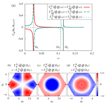
Figure 9: The four-point vertex function solved by discretizing Eq. (49) on $60\times 60$ uniform mesh. The parameters are fixed at $J=\zeta=1,D=2.808$. (a) Energy dependence of $\Gamma_{\bm{q}}$ in three dominant scattering channels. The positions of the poles are denoted as $\Omega_{\nu}$ in the figure. (b)–(d) Momentum dependence of $\Gamma_{\bm{q}}$ at the poles $\Omega_{\nu}+\epsilon$, where $\epsilon\rightarrow+0$.

The two-particle propagator near the pole $\omega=\Omega_{\nu}$ ($\nu=1,2,3$) has the form  Nakanishi (1969); Ueda and Momoi (2013):

$$\quad G^{(2)}(\omega,\bm{K}=\bm{k}_{1}+\bm{k}_{2},\frac{\bm{k}_{1}-\bm{k}_{2}}{2},\frac{\bm{k}_{1}-\bm{k}_{2}}{2}+\bm{q})$$

$$\approx\frac{\langle 0|\gamma_{\bm{k}_{1}+\bm{q}\uparrow}\gamma_{\bm{k}_{2}-\bm{q}\downarrow}|\Psi^{(\nu)}\rangle\langle\Psi^{(\nu)}|\gamma_{\bm{k}_{1}\uparrow}^{\dagger}\gamma_{\bm{k}_{2}\downarrow}^{\dagger}|0\rangle}{\omega-\Omega_{\nu}}$$

$$=\frac{\Psi_{\bm{K}}^{(\nu)}(\frac{\bm{k}_{1}-\bm{k}_{2}}{2}+\bm{q})\Psi_{\bm{K}}^{(\nu)*}(\frac{\bm{k}_{1}-\bm{k}_{2}}{2})}{\omega-\Omega_{\nu}},$$ (51)

where $\Psi_{\bm{K}}^{(\nu)}(\bm{k})$ is the two-particle wave function with total momentum $\bm{K}$ and relative momentum $\bm{k}$.

Alternatively, we can obtain this two-particle propagator from the self-energy corrections. Near the pole at $\omega=\Omega_{\nu}$,

$$\quad G^{(2)}(\omega,\bm{K},\frac{\bm{k}_{1}-\bm{k}_{2}}{2},\frac{\bm{k}_{1}-\bm{k}_{2}}{2}+\bm{q})$$

$$\approx G_{0}^{(2)}(\Omega_{\nu},\bm{K},\frac{\bm{k}_{1}-\bm{k}_{2}}{2})$$

$$\quad\times\Gamma_{\bm{q}}^{N}(\bm{k}_{1},\bm{k}_{2},\Omega_{\nu})\cdot G_{0}^{(2)}(\Omega_{\nu},\bm{K},\frac{\bm{k}_{1}-\bm{k}_{2}}{2}+\bm{q}).$$ (52)

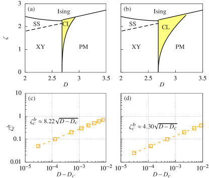
Figure 10: (a), (b): Phase diagram of the XXZ model with single-ion anisotropy Eq. (1). The CL/PM phase boundary is obtained by solving the BS equation Eq. (49) on a non-uniform mesh, where more points are sampled near the singular part of the interactions until convergence. The Ising/PM, Ising/SS, and SS/XY phase boundaries are discussed in Appendix A. In (a) we used the solution of Eq. (49) with only normal interactions present. In (b) we used the full solution of Eq. (49). (c), (d) The chiral phase boundaries in log-log scale for panels (a) and (b), respectively.

Combining Eqs. (III.5) and (III.5), we can connect the symmetry of four-point interaction vertices to the symmetry of two-particle wave functions:

$$\frac{\Gamma^{N}_{\bm{Q}+\bm{q}}(\bar{\bm{Q}},\bm{Q},\Omega_{\nu})}{\Gamma^{N}_{\bm{Q}-\bm{q}}(\bar{\bm{Q}},\bm{Q},\Omega_{\nu})} =\frac{\Psi_{\bm{K}=0}^{(\nu)}(\bm{q})}{\Psi_{\bm{K}=0}^{(\nu)}(-\bm{q})},$$ (53a)

$$\frac{\Gamma^{N}_{\bm{q}}(\bm{Q},\bm{Q},\Omega_{\nu})}{\Gamma^{N}_{-\bm{q}}(\bm{Q},\bm{Q},\Omega_{\nu})} =\frac{\Psi_{\bm{K}=2\bm{Q}}^{(\nu)}(\bm{q})}{\Psi_{\bm{K}=2\bm{Q}}^{(\nu)}(-\bm{q})}.$$ (53b)

From these relations we can extract the symmetry of the bound-state wave functions:

$$\Psi_{\bm{K}=0}^{(1)}(\bm{q}) =-\Psi_{\bm{K}=0}^{(1)}(-\bm{q}),$$ (54a)

$$\Psi_{\bm{K}=0}^{(2)}(\bm{q}) =\quad\Psi_{\bm{K}=0}^{(2)}(-\bm{q}),$$ (54b)

$$\Psi_{\bm{K}=2\bm{Q}}^{(3)}(\bm{q}) =\quad\Psi_{\bm{K}=2\bm{Q}}^{(3)}(-\bm{q}).$$ (54c)

We found that out of three bound-state frequencies, the smallest one is $\Omega_{1}$. We see from (54a) that the corresponding wavefunction is odd under spatial inversion, consistent with the symmetry of the chiral order parameter $\kappa$.

When $\zeta$ increases at a constant $D$, or $D$ decreases at a constant $\zeta$, the attractive interaction between bosons with opposite flavors also increases, and the bound-state frequency $\Omega_{1}$ decreases and eventually reaches zero. The softening of the $\Omega_{1}$ mode signals the onset of the CL phase.

We show the location of the transition into the CL phase in Fig. 10. The solid line between CL/PM in Fig. 10a shows the location of the boundary of the CL phase, obtained numerically by keeping in the BS equation  (49) only the normal interaction $V^{22o}$ (i.e., only particle number conserving processes). Figure 10b shows the location of the CL phase boundary obtained by solving the full Eq. (49), keeping both $V^{22o}$ and $V^{40},V^{04}$ interactions. In both cases, the phase boundary is obtained by requiring that the pole frequency is zero, $\Omega_{1}=0$.

Although the analysis in this section is justified when $D^{b}_{c}$ is substantially larger than $D_{c}$, which requires $\zeta$ of order one, it is nevertheless useful to compare the results of this and the previous sections. In the previous Sec. III.4, we found that the instability towards CL state at small $\zeta$ is related to singular behavior of the dressed pairing interaction, which scales as $\zeta^{2}/\omega_{\bm{Q}}^{2}$. A naive discretization of Eq. (49) using a uniform mesh of $210\times 210$ points in the first BZ does not capture the singular part of the interaction. To obtain the boundary of the CL phase at small $\zeta$, we used a non-uniform mesh which is much denser near the singular region of Eq. (49). The phase diagrams shown in Fig. 10 were verified by sampling $\sim 5000$ points near $\bm{q}=\{0,2\bm{Q}\}$ on top of a $30\times 30$ uniform background.

To further compare the results obtained to second order in $J_{z}$ with the ones obtained by solving BS equation, we label by $\alpha$ the overall numerical factor from the second-order diagrams. The full second-order result, Eq. (45), gives $\alpha=2.49$. If instead we pick only normal forward scattering process from forward scattering normal vertices [diagram (a) in Fig. 6], we obtain $\alpha\approx 0.33$. If we added up all ladder contributions [diagrams (a) and (b) in Figs. 6 and 7], we would obtain larger $\alpha\approx 1.34$. Observe that larger $\alpha$ leads, at fixed $\zeta$, to larger critical $D^{b}_{c}$ [see Eq. (48)]. This is consistent with the results obtained by solving BS equation, Fig. 10. We recall that if we use all second order diagrams, we obtain an even larger $\alpha\approx 2.49$. This means that using only ladder diagrams in the BS equation gives a conservative estimate of the critical $D^{b}_{c}$ for the instability towards the CL state. In Figs. 10(c) and 10(d), the critical scaling of the chiral phase boundary is found to be $\zeta_{c}^{b}\sim\left(D_{c}^{b}-D_{c}\right)^{1/2}$, again in agreement with the $J_{z}^{2}$ analysis in the previous section.

IV DMRG calculation of the single- and two-magnon gaps

To provide further evidence that the two-magnon bound-state gap $\Delta_{b}$ closes before closing the single-magnon gap $\Delta_{s}$ upon decreasing $D$, we perform density matrix renormalization group (DMRG) calculations on $6\times 6$ triangular lattice with periodic boundary condition . $M=6000$ states were kept in the calculation, leading to truncation error $<10^{-4}$ for all the data points presented here.

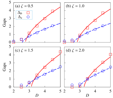
Figure 11: Two-magnon gap $\Delta_{b}$ and single-magnon gap $\Delta_{s}$ obtained from DMRG on $6\!\times\!6$ triangular lattice with periodic boundary condition, with $J=1$. The solid (dashed) line represents fitting to the gap $\Delta_{b}$ ($\Delta_{s}$) by Eq. (55) with two parameters $\{c_{b},\,D_{b}\}$ ($\{c_{s},\,D_{s}\}$). Only data points before gap crossing are used in the fitting procedure.

In DMRG, the two-magnon gap $\Delta_{b}$ (single-magnon gap $\Delta_{s}$) corresponds to the energy of the first excited state in the $S_{z}=0$ sector (ground state in the $S_{z}=1$ sector), measured from the $S_{z}=0$ ground state. Since the transition into the CL phase belongs to the $d=3$ Ising university class, the critical exponent $\nu$ is given by $\nu_{\text{Ising}}\approx 0.63$. Similarly, the transition into XY phase belongs to $d=3$ XY university class, giving $\nu_{\text{XY}}\approx 0.67$:

$$\Delta_{b} =E_{S_{z}=0}^{(1)}-E_{S_{z}=0}^{(0)}=c_{b}(D-D_{b})^{\nu_{\text{Ising}}},$$ (55a)

$$\Delta_{s} =E_{S_{z}=1}^{(0)}-E_{S_{z}=0}^{(0)}=c_{s}(D-D_{s})^{\nu_{\text{XY}}},$$ (55b)

where the superscripts $(0)$ and $(1)$ denote the ground and the first excited state, respectively.

In Fig. 11, we calculate the evolution of the two gaps as a function of $D$, for four different values of $\zeta=\{0.5,1.0,1.5,2.0\}$. The data are then fitted to Eq. (55) with two fitting parameters (while keeping $\nu$ fixed to the known value). In all cases, the two gaps clearly cross each other before closing, indicating that the VC order emerges before single-particle excitations of the paramagnetic state soften.

As discussed in previous sections, the first excitation in the $S_{z}=0$ sector is odd under inversion, and its condensation signals the appearance of the VC order. This can be checked numerically: by performing an exact diagonalization on $3\times 3$ and $3\times 6$ lattices, we can obtain the wave function of the lowest-energy states. The first excited state in the $S_{z}=0$ sector is always found to be odd under inversion.

V Conclusions

In this work, we studied the sequence of quantum phase transitions in the spin-$1$ triangular XXZ model, induced by an easy-plane single-ion anisotropy $D$ (see Fig. 1). Within non-interacting magnon approximation, the system is in a paramagnetic state at $D>D_{c}$ and in the XY-ordered phase at $D<D_{c}$. We analyzed the effects of interactions and found that they change the phase diagram in a qualitative way. Namely, we found that the continuous U(1) symmetry and the discrete chiral Z₂ symmetry, which are spontaneously broken in the XY ordered phase, break at different values $D$, implying the existence of an intermediate chiral liquid phase in-between the XY and quantum paramagnetic phases. This liquid phase has no magnetic ordering ($\langle\bm{S}_{n}\rangle=0$) and is characterized by a finite staggered vector chirality, $\langle{\kappa}_{nm}\cdot{\hat{\bm{z}}}\rangle\neq 0$, which has opposite sign on the neighboring triangles. It therefore spontaneously breaks spatial inversion symmetry. Note that the time-reversal symmetry is preserved. Our analytical results are supported by DMRG simulations on a $6\times 6$ triangular lattice. Remarkably, we find the gapped chiral liquid phase to extend up to large values of the exchange anisotropy ($\zeta>2$), for which its window of stability reaches $D_{c}^{b}-D_{c}\simeq J/2$. This rather large range of stability opens the possibility of observing this phase in real materials.

As we discussed in the Introduction, this is not the first time an Ising-type phase with nematic order parameter bilinear in microscopic spin degrees of freedom is observed. However, the previous and closely related observations Chubukov and Starykh (2013); Parker and Balents (2017), involved semiclassical large spin ($S\gg 1$) expansion of Heisenberg models with pronounced spatial anisotropy subject to external magnetic field on triangular and kagomé lattices, correspondingly. Our consideration is specific to a more ‘quantum’ spin $S=1$ and spatially isotropic triangular lattice model and does not require an external magnetic field.

The experimental signatures of the VC order have been discussed in Refs. Chubukov and Starykh (2013); Parker and Balents (2017) They are related to the so-called “inverse Dzyaloshinskii-Moriya (DM)” effect, which was proposed as a mechanism for multi-ferroic behavior of spiral magnets Katsura et al. (2005); Sergienko and Dagotto (2006); Mostovoy (2006). Namely, a local VC order parameter $\langle\bm{S}_{j}\times\bm{S}_{l}\rangle$ produces a net electric dipole proportional to $\bm{e}_{jl}\times\langle\bm{S}_{j}\times\bm{S}_{l}\rangle$ (where $\bm{e}_{jl}\equiv({\bm{r}}_{j}-{\bm{r}}_{l})/|{\bm{r}}_{j}-{\bm{r}}_{l}|$). As shown in Fig. 12, the polarization is induced by the displacement $\delta\bm{r}$ of a medium ion (with charge $q_{I}$) away from the bond center. This ion is typically an anion ($q_{I}<0$), e.g., oxygen O^2- for the case of transition metal oxides, and it mediates the super-exchange interaction between spins $\bm{S}_{j}$ and $\bm{S}_{l}$. The induced DM interaction, ${\bm{D}}_{jl}\propto\delta\bm{r}\times{\bm{e}}_{jl}$, lowers the magnetic energy by $\bm{D}_{jl}\cdot\langle\bm{S}_{j}\times\bm{S}_{l}\rangle$, which is linear in $\delta\bm{r}$. Because the elastic energy cost is quadratic in $\delta\bm{r}$, the local electric polarization $q_{I}\delta{\bm{r}}$ becomes finite once $\langle\bm{S}_{j}\times\bm{S}_{l}\rangle\neq 0$. As it is clear from Fig. 12, the ionic displacements induced by the staggered VC ordering lead to a charge density wave order, which can be detected with x rays.

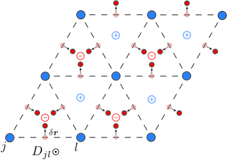
Figure 12: Schematic plot of the inverse Dzyaloshinskii-Moriya effect.

It is worth stressing once again that geometric frustration is essential to our construction: spontaneous breaking of the inversion symmetry occurs via formation of the two-magnon bound state formed by magnons at $\pm{\bm{Q}}$ which are degenerate in energy. Similar considerations apply to lattice models of strongly interacting bosons Zaletel et al. (2014); Janzen et al. (2016); Zhu et al. (2016) with inverted (frustrated) sign of particle’s hopping between sites. There is a certain similarity between our results and loop current orders proposed for strongly correlated fermion models Simon and Varma (2002); Wang and Chubukov (2014); Agterberg et al. (2015).

From a statistical physics perspective, we can think of this quantum phase a transition as a classical phase transition in dimension $2+1$. It is known that the suppression of XY ordering is induced by proliferation of vortex lines that span the full system Kleinert (1989). In the paramagnetic state, vortex and anti-vortices have the same probability of being at a given triangle. In the chiral liquid state, the vortices occupy one sublattice of triangles (e.g., the triangles that are pointing up) with higher probability, while anti-vortices occupy the other sublattice (e.g., the triangles that are pointing down) with higher probability. In other words, the staggered chiral liquid is a vortex density wave.

Finally, it is important to note that our conclusions are far more general than the particular model that we have considered here. Our results suggest that exotic quantum liquid states are likely to emerge in the proximity of quantum phase transitions between a $T=0$ paramagnet and quantum magnet that breaks both continuous and discrete symmetries. In other words, like in the case of metallic systems where quantum critical points guide the experimental search for unconventional superconductors and non-Fermi-liquid behavior, the quantum critical points of bosonic systems can play a similar role in the experimental search for exotic quantum liquids.

VI Acknowledgements

We thank Z. Nussinov, Y. Motome, and S. Zhang for helpful discussions. The numerical results were obtained in part using the computational resources of the National Energy Research Scientific Computing Center, which is supported by the Office of Science of the U.S. Department of Energy under Contract No. DE-AC02-05CH11231. Z.W. and C.D.B. are supported by funding from the Lincoln Chair of Excellence in Physics and from the Los Alamos National Laboratory Directed Research and Development program. O.A.S. is supported by the National Science Foundation Grant No. NSF DMR-1507054. W.Z. is supported by DOE NNSA through LANL LDRD program. A.V.C. is supported by Grant No. NSF DMR-1523036.

Appendix A Other phases of the model

Here, we discuss the additional phases that appear in our model for large enough $J_{z}$. As shown in Fig. 10, the PM and CL phases are bounded from above by an Ising-type spin density wave (SDW) phase, which becomes the ground state for strong enough $\zeta J$. This phase, which is described by the local SDW order parameter $\langle S^{z}_{\bm{r}}\rangle\propto e^{i{\bm{Q}}\cdot{\bm{r}}}$, corresponds to a three-sublattice ordering with $\langle S^{z}_{\bm{r}}\rangle$ being positive in one sublattice (A), negative in another sublattice (B), and equal to zero (disordered) on the third sublattice (C). This partially disordered AFM ordering is obtained for the triangular lattice $S=1$ Blume-Capel model Blume (1966); Capel (1966); Blume et al. (1971); Mahan and Girvin (1978); Collins et al. (1988), which is obtained by setting the $XY$ exchange to zero in our Hamiltonian ${\cal H}$ defined in Eq. (1).

At mean-field level, there is an intermediate phase preempting the transition between the Ising and XY phases. This phase is characterized by coexistence of Ising-type SDW and in-plane magnetic ordering [which breaks U(1) symmetry] known as spin supersolid (SS) state Penrose and Onsager (1956); Ng and Lee (2006); Laflorencie and Mila (2007); Sengupta and Batista (2007a, b); Picon et al. (2008); Peters et al. (2009). The SS phase is also a three-sublattice ordering, whose longitudinal components follow the same pattern as in the partially disordered Ising phase, while the transverse components form a collinear pattern

$$S_{\bm{r}_{A}}^{\perp}=S_{\bm{r}_{B}}^{\perp}=-\alpha S_{\bm{r}_{C}}^{\perp},$$ (56a)

$$S_{\bm{r}_{A}}^{z}=-S_{\bm{r}_{B}}^{z}\neq 0,~{}~{}S_{\bm{r}_{C}}^{z}=0,$$ (56b)

where $\alpha<1$. The collinear ordering is more favorable than the $120\degree$ structure because of the different magnitudes of transverse spin components.

The boundary between the partially disordered Ising phase and the PM phase is determined by comparing their ground state energies. The ground state energy of the PM phase is given in Eq. (25). The ground-state energy of the partially disordered Ising phase can be computed by using the same Lagrange multiplier method that we applied to the quantum PM.

The spin operators are again represented by SU(3) Schwinger bosons in the fundamental representation [see Eqs. (15)–(III.1)]. The mean-field state of the Ising phase corresponds to condensation of different flavors of bosons in three sublattices:

$$b_{\bm{r}_{A}\uparrow}^{\dagger}=s_{1},\quad b_{\bm{r}_{B}\downarrow}^{\dagger}=s_{-1},\quad b_{\bm{r}_{C}0}^{\dagger}=s_{0}.$$ (57)

Due to time-reversal symmetry, we expect $s_{1}=s_{-1}$, and $\mu_{1}=\mu_{-1}$. The spin-wave Hamiltonian is

$$\bar{\mathcal{H}}_{sw} =\sum_{\bm{k}}\Big{[}\Psi_{\bm{k}}^{\dagger}\bar{H}_{sw}(\bm{k})\Psi_{\bm{k}}+(3s_{1}^{2}\zeta J+D+\mu_{1})$$

$$\quad\qquad\times\left(b_{A\downarrow,\bm{k}}^{\dagger}b_{A\downarrow,\bm{k}}+b_{B\uparrow,\bm{k}}^{\dagger}b_{B\uparrow,\bm{k}}\right)\Big{]}$$

$$\quad+\frac{N}{3}\Big{[}(s_{0}^{2}-2)\mu_{0}+(2s_{1}^{2}-3)\mu_{1}$$

$$\quad\qquad+(2s_{1}^{2}-1)D-3s_{1}^{4}\zeta J\Big{]},$$ (58)

where

$$\Psi_{\bm{k}}\equiv\begin{pmatrix}b_{A0,\bm{k}}&b_{C\downarrow,\bm{k}}&b_{B0,\bar{\bm{k}}}^{\dagger}&b_{C\uparrow,\bar{\bm{k}}}^{\dagger}\end{pmatrix}^{T},$$ (59)

and the $4\times 4$ matrix $\bar{H}_{sw}(\bm{k})$ is:

$$\bar{H}_{sw}(\bm{k})\!=\!\begin{pmatrix}\mu_{1}&s_{0}s_{1}\Gamma_{\bar{\bm{k}}}&s_{1}^{2}\Gamma_{\bm{k}}&s_{0}s_{1}\Gamma_{\bar{\bm{k}}}\\ s_{0}s_{1}\Gamma_{\bm{k}}&\mu_{0}+D&s_{0}s_{1}\Gamma_{\bar{\bm{k}}}&0\\ s_{1}^{2}\Gamma_{\bar{\bm{k}}}&s_{0}s_{1}\Gamma_{\bm{k}}&\mu_{1}&s_{0}s_{1}\Gamma_{\bm{k}}\\ s_{0}s_{1}\Gamma_{\bm{k}}&0&s_{0}s_{1}\Gamma_{\bar{\bm{k}}}&\mu_{0}+D\end{pmatrix},$$ (60)

with $\Gamma_{\bm{k}}\equiv J\sum_{\nu}\exp(-i\bm{k}\cdot\bm{e}_{\nu})$.

By diagonalizing the matrix $\text{diag}\{1,1,-1,-1\}\bar{H}_{sw}(\bm{k})$ we obtain the ground-state energy:

$$E_{0}^{\text{Ising}} =\frac{1}{N}\sum_{\bm{k}}\left(\omega_{+,\bm{k}}+\omega_{-,\bm{k}}\right)+\frac{1}{3}\Big{[}(s_{0}^{2}-2)\mu_{0}$$

$$\quad+(2s_{1}^{2}-3)\mu_{1}+(2s_{1}^{2}-1)D-3s_{1}^{4}\zeta J\Big{]},$$ (61)

where

$$\omega_{\pm,\bm{k}}=\frac{1}{\sqrt{2}}\sqrt{\tau_{\bm{k}}\pm\sqrt{\kappa_{\bm{k}}}}.$$ (62)

$$\tau_{\bm{k}} =(D+\mu_{0})^{2}+\mu_{1}^{2}-s_{1}^{4}\left|\Gamma_{\bm{k}}\right|^{2},$$ (63a)

$$\kappa_{\bm{k}} =-4\mu_{1}^{2}(D+\mu_{0})^{2}-4s_{1}^{2}(D+\mu_{0})\Big{[}2s_{0}^{2}s_{1}^{2}\left(\Gamma_{\bm{k}}^{3}+\Gamma_{\bar{\bm{k}}}^{3}\right)$$

$$\quad-\left|\Gamma_{\bm{k}}\right|^{2}\left(4s_{0}^{2}\mu_{1}+s_{1}^{2}(D+\mu_{0})\right)\Big{]}+\tau_{\bm{k}}^{2}.$$ (63b)

The variational parameters $\{s_{0},s_{1},\mu_{0},\mu_{1}\}$ are obtained from the saddle point equations

$$\frac{\partial E_{0}^{\text{Ising}}}{\partial s_{0}}=0,\,\frac{\partial E_{0}^{\text{Ising}}}{\partial s_{1}}=0,\,\frac{\partial E_{0}^{\text{Ising}}}{\partial\mu_{0}}=0,\,\frac{\partial E_{0}^{\text{Ising}}}{\partial\mu_{1}}=0.$$ (64)

For large $\zeta$, the energy $E_{0}^{\text{Ising}}$ becomes lower than $E_{0}^{\text{PM}}$, corresponding to a first order phase transition between the quantum PM phase and the partially disordered Ising phase. The transition line, shown in Fig. 10, is determined by solving the equation $E_{0}^{\text{Ising}}=E_{0}^{\text{PM}}$.

Now, we discuss the phase transition from the partially disordered Ising phase to the SS phase. This transition is characterized by spontaneous U(1) symmetry breaking due to the emergence of the in-plane component. The continuous transition is then determined from the softening of the low-energy modes of the partially disordered Ising phase: $\omega_{-,\pm\bm{Q}}=0$. The resulting phase boundary corresponds to the solid line in Fig. 10.

The phase boundary between the XY and SS phases is denoted with a dashed line in Fig. 10. We note that this particular phase boundary is calculated only at the mean-field level Papanicolaou (1988); Penc and Läuchli (2011). The mean-field treatment is carried out by minimizing the energy with respect to the variational wave function $|\Psi\rangle=\otimes_{\bm{r}}|\bm{d}_{\bm{r}}\rangle$, where

$$|\bm{d}_{\bm{r}}\rangle=\frac{id_{\bm{r}}^{x}+d_{\bm{r}}^{y}}{\sqrt{2}}|\uparrow\rangle_{\bm{r}}+\frac{-id_{\bm{r}}^{x}+d_{\bm{r}}^{y}}{\sqrt{2}}|\downarrow\rangle_{\bm{r}}-id_{\bm{r}}^{z}|0\rangle_{\bm{r}}.$$ (65)

Up to a U(1) rotation, the variational mean-field state for the XY phase is:

$$\bm{d}_{\bm{r}_{A}} =\left(0,\,-i\sin\frac{a}{2},\,\cos\frac{a}{2}\right),$$ (66a)

$$\bm{d}_{\bm{r}_{B}} =\left(\frac{i\sqrt{3}}{2}\sin\frac{a}{2},\,\frac{i}{2}\sin\frac{a}{2},\,\cos\frac{a}{2}\right),$$ (66b)

$$\bm{d}_{\bm{r}_{C}} =\left(\frac{-i\sqrt{3}}{2}\sin\frac{a}{2},\,\frac{i}{2}\sin\frac{a}{2},\,\cos\frac{a}{2}\right),$$ (66c)

which leads to

$$E_{0}^{\text{XY}}=-\frac{3J}{2}\sin^{2}a+D\sin^{2}\frac{a}{2}.$$ (67)

Minimization of $E_{0}^{\text{XY}}$ with respect to $a$ gives

$$E_{0}^{\text{XY}}=\frac{D}{2}-\frac{3J}{2}-\frac{D^{2}}{24J}.$$ (68)

Up to a U(1) rotation, the variational mean-field state for the SS phase is:

$$\bm{d}_{\bm{r}_{A}} =\left(\cos\frac{a}{2},\,i\sin\frac{a}{2}\cos b,\,i\sin\frac{a}{2}\sin b\right),$$ (69a)

$$\bm{d}_{\bm{r}_{B}} =\left(-\cos\frac{a}{2},\,i\sin\frac{a}{2}\cos b,\,-i\sin\frac{a}{2}\sin b\right),$$ (69b)

$$\bm{d}_{\bm{r}_{C}} =\left(i\sin\frac{c}{2},\,0,\,\cos\frac{c}{2}\right),$$ (69c)

leading to

$$E_{0}^{\text{SS}} =J\left(\sin a\sin b-\sin c\right)^{2}-J\sin^{2}c-\zeta J\sin^{2}a\cos^{2}b$$

$$\quad+\frac{D}{3}\left(2\cos^{2}\frac{a}{2}+2\sin^{2}\frac{a}{2}\cos^{2}b+\sin^{2}\frac{c}{2}\right).$$ (70)

The minimum of $E_{0}^{\text{SS}}$ as a function of the three independent variatonal parameters is obtained numerically. The phase boundary between XY and SS phase results from the condition $E_{0}^{\text{XY}}=E_{0}^{\text{SS}}$ (see the dashed line in Fig. 10).

Appendix B A complementary approach using hard-core bosons

In this appendix we discuss a complementary approach to the CL problem, which uses somewhat different transformation to hard-core bosons for $S=1$, but at the end leads to the same results as the approach used in the main text.

Namely, we represent spin operators at a given site via two Bose operators $a$ and $b$  Chubukov (1989, 1990b); Chubukov et al. (1991); Chubukov and Morr (1995)

$$S_{z} =-i\left(a^{\dagger}b-b^{\dagger}a\right),$$ (71a)

$$S_{x} =-i\left(b^{\dagger}U-Ub\right),$$ (71b)

$$S_{y} =-i\left(Ua-a^{\dagger}U\right),$$ (71c)

where $U=\left(1-a^{\dagger}a-b^{\dagger}b\right)^{1/2}$. The $a$ and $b$ bosons at every lattice site obey the constraint $a^{\dagger}a+b^{\dagger}b=0,1$. With this extra condition, spin commutation relations are satisfied, and

$$S^{2}_{z} =a^{\dagger}a+b^{\dagger}b,$$ (72a)

$$S^{2}_{x} =1-a^{\dagger}a,$$ (72b)

$$S^{2}_{y} =1-b^{\dagger}b,$$ (72c)

such that ${\bm{S}}^{2}=2$, as it should be.

The Hamiltonian of Eq. (1) is expressed via $a$ and $b$ bosons as

$${\cal H}={\cal H}_{2}+{\cal H}_{4},$$ (73)

where in momentum space

$${\cal H}_{2} =\sum_{\bm{k}}\left[\left(D+\epsilon_{\bm{k}}\right)a^{\dagger}_{\bm{k}}a_{\bm{k}}-\frac{\epsilon_{\bm{k}}}{2}\left(a^{\dagger}_{\bm{k}}a^{\dagger}_{-{\bm{k}}}+a_{\bm{k}}a_{-{\bm{k}}}\right)\right]$$

$$+\sum_{\bm{k}}\left[\left(D+\epsilon_{\bm{k}}\right)b^{\dagger}_{\bm{k}}b_{\bm{k}}-\frac{\epsilon_{\bm{k}}}{2}\left(b^{\dagger}_{\bm{k}}b^{\dagger}_{-{\bm{k}}}+b_{\bm{k}}b_{-{\bm{k}}}\right)\right],$$ (74)

and

$${\cal H}_{4} =\frac{J_{z}}{N}\sum_{{\bm{k}}_{i}}a^{\dagger}_{{\bm{k}}_{1}}b^{\dagger}_{{\bm{k}}_{2}}b_{{\bm{k}}_{3}}a_{{\bm{k}}_{4}}\left(\gamma_{{\bm{k}}_{1}-{\bm{k}}_{3}}+\gamma_{{\bm{k}}_{2}-{\bm{k}}_{4}}\right)$$

$$-\frac{J_{z}}{2N}\sum_{{\bm{k}}_{i}}\left(a^{\dagger}_{{\bm{k}}_{1}}a^{\dagger}_{{\bm{k}}_{2}}b_{{\bm{k}}_{3}}b_{{\bm{k}}_{4}}+b^{\dagger}_{{\bm{k}}_{1}}b^{\dagger}_{{\bm{k}}_{2}}a_{{\bm{k}}_{3}}a_{{\bm{k}}_{4}}\right)\times$$

$$\quad\left(\gamma_{{\bm{k}}_{1}-{\bm{k}}_{3}}+\gamma_{{\bm{k}}_{1}-{\bm{k}}_{4}}\right).$$ (75)

Here, $\epsilon_{\bm{k}}=2J\gamma_{\bm{k}}$ and $\gamma_{\bm{k}}=\sum_{\nu}\cos{{\bm{k}}\cdot{\bm{e}}_{\nu}}$. There is no four-boson term from the transverse, $J$, part of the spin-spin interaction, once the constraint is satisfied.

Because the boson density $a^{\dagger}a+b^{\dagger}b$ can have two values at a given site, there is no straightforward way to enforce the constraint by introducing the Lagrange multiplier. One can either extend the model to $N>1$ bosonic flavors and expand in $1/N$, or just assume that the average density of bosons is small and neglect the constraint. The last approach is rigorously justified only at large $D\gg J$, but we expect that it gives meaningful results also at $D\geq J$, as long as single-particle spin-wave excitations are gapped. Below we just neglect the constraint and analyze the formation of the two-particle bound state within the model of Eqs. (B) and (B) with no additional constraint. We recall in this regard that within the Schwinger boson approach, which we adopted in the main text, we replaced one bosonic field, $b_{0}$, by its condensate value $s$ and thereby also reduced the model to that of two interacting bosonic fields. The site-independent Lagrange multiplier $\mu$, which we introduced in the main text to enforce the constraint, and the condensate $s$ renormalize $D$ and $J$ in the quadratic form, but do not affect its structure. From this perspective, the Hamiltonian of Eqs. (B) and (B) is qualitatively the same as the one in the main text, assuming that one adjusts $D$ and $J$.

Furthermore, one can show that the transformation from operators $b_{\uparrow}$ and $b_{\downarrow}$ of the main text to operators $a$ and $b$ used here is just a rotation in operator space:

$$a=\frac{b_{\downarrow}-b_{\uparrow}}{\sqrt{2}},~{}~{}~{}b=(-i)\frac{b_{\uparrow}+b_{\downarrow}}{\sqrt{2}}$$ (76)

Obviously then, the results obtained using $a$ and $b$ bosons must be equivalent to those obtained using $b_{\uparrow}$ and $b_{\downarrow}$ bosons. We will see, however, that technical details of the computation of the bound-state instability differ between the approaches.

We now proceed with the Hamiltonian of Eqs. (B) and (B). The diagonalization of the quadratic form in (B) is done in the usual way. We introduce

$$a_{\bm{k}}=u_{\bm{k}}d_{\bm{k}}-v_{\bm{k}}d^{\dagger}_{-{\bm{k}}},~{}~{}b_{\bm{k}}=u_{\bm{k}}{\bar{d}}_{\bm{k}}-v_{\bm{k}}{\bar{d}}^{\dagger}_{-{\bm{k}}}$$ (77)

and choose

$$u_{\bm{k}} =(D+\omega_{\bm{k}})/(2\sqrt{D\omega_{\bm{k}}}),$$ (78a)

$$v_{\bm{k}} =(D-\omega_{\bm{k}})/(2\sqrt{D\omega_{\bm{k}}}),$$ (78b)

$$\omega_{\bm{k}} =\sqrt{A^{2}_{\bm{k}}-B^{2}_{\bm{k}}}=\sqrt{D^{2}+2D\epsilon_{\bm{k}}},$$ (78c)

where

$$A_{\bm{k}}=D+\epsilon_{\bm{k}},~{}~{}B_{\bm{k}}=-\epsilon_{\bm{k}}.$$ (79)

The spin-wave spectrum softens at ${\bm{k}}=\pm{\bm{Q}}=\pm(4\pi/3,0)$ at $D_{c}=6J$. In the main text, we found $D_{c}=2.68J$, which is in better agreement with the numerics. We recall that the result was obtained by including one-loop renormalizations of $D$ and $J$. Here, we neglect these renormalizations. $D_{c}=6J$ would be the critical value in the Schwinger boson analysis, presented in the main text, if we set $s=1$ and $\mu=D$ there.

Note that (79) predicts that at the minimum of the magnon dispersion $\omega_{\bm{Q}}\sim\sqrt{D-D_{c}}$ while for Schwinger bosons the relation is linear [see discussion below Eq. (48)].

One can easily verify that the two-particle order parameter, which leads to a spin current state with a non-zero vector chirality $\kappa_{mn}$, has zero total momentum and is expressed in terms of $a$ and $b$ bosons as

$$\langle b_{\bm{p}}a_{-{\bm{p}}}\rangle=i{\tilde{\Phi}}_{|{\bm{p}}|}f_{\bm{p}},~{}~{}\langle b^{\dagger}_{\bm{p}}a^{\dagger}_{-{\bm{p}}}\rangle=-i{\tilde{\Phi}}_{|{\bm{p}}|}f_{\bm{p}},$$ (80)

where $f_{-{\bm{p}}}=-f_{{\bm{p}}}$ is an odd function of momentum, normalized to $f_{\bm{Q}}=1,f_{-{\bm{Q}}}=-1$. The vector chirality on $m,n$ bond is $\kappa_{m,n}\propto\sum_{\bm{p}}{\tilde{\Phi}}_{{\bm{p}}}$. In terms of bosons $d_{k}$ and ${\bar{d}}_{k}$ [Eq. (77)], the VC order parameter is expressed as

$$\langle{\bar{d}}_{\bm{p}}d_{-{\bm{p}}}\rangle =i\Phi_{|{\bm{p}}|}f_{\bm{p}},$$ (81a)

$$\langle{\bar{d}}^{\dagger}_{\bm{p}}d^{\dagger}_{-{\bm{p}}}\rangle =-i\Phi_{|{\bm{p}}|}f_{\bm{p}},$$ (81b)

where $\Phi_{|{\bm{p}}|}={\tilde{\Phi}}_{|{\bm{p}}|}\omega_{\bm{p}}/A_{\bm{p}}$. Note that both $\omega_{\bm{p}}$ and $A_{\bm{p}}$ are even functions of ${\bm{p}}$.

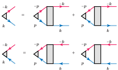
Figure 13: Equations for the vertices $\Phi_{|{\bm{p}}|}$. The triangular vertices denote $i\Phi_{|{\bm{p}}|}$ for ${\bm{p}}$ near ${\bm{Q}}$ and $-i\Phi_{|{\bm{p}}|}$ for ${\bm{p}}$ near ${-\bm{Q}}$, or $-i\Phi_{|{\bm{p}}|}$ for ${\bm{p}}$ near ${\bm{Q}}$ and $i\Phi_{|{\bm{p}}|}$ for ${\bm{p}}$ near ${-\bm{Q}}$, depending on the direction of arrows. Solid and double solid lines denote propagators of $d$ and ${\bar{d}}$ magnons, and the shaded rectangles denote fully dressed irreducible interactions between low-energy magnons.

We now search for the two-particle instability at $D>D_{c}$, i.e., preemptying to the spin-wave instability. Like in the main text, we consider small $J_{z}=\zeta J$. The analysis of the two-particle instability proceeds in the same way as in Sec. III.3. Namely, we write self-consistent equations on $\Phi_{|{\bm{p}}|}$ in terms of the fully renormalized irreducible pairing interaction between $d$ and ${\bar{d}}$ bosons with opposite momenta near $\pm{\bm{Q}}$.

The equation for the two-particle vertex is graphically presented in Fig. 13. It is quite similar to Fig. 4 in the main text, but now the shaded triangular vertices denote $\Phi_{|{\bm{p}}|}$, solid single and double lines describe propagators of $d$ and ${\bar{d}}$ bosons, and the shaded four-point vertices represent fully dressed irreducible interactions.

Like we said in the main text, the distinction between our problem and superconductivity is in that boson-boson interaction does not conserves the number of bosons; the interaction Hamiltonian, re-expressed in terms of bosons $d_{\bm{k}}$ and ${\bar{d}}_{\bm{k}}$, contains terms which create two bosons and annihilate two bosons, and also terms which create or annihilate four bosons (as well as the terms which create three bosons and annihilate one, and vice versa). Accordingly, the right-hand side of the equation for $\Phi$ contains both normal and “anomalous” terms (direction of the internal lines is the same or opposite to the direction of external lines). At the same time, the internal part of both terms contains propagators of one $d_{\bm{k}}$ and one ${\bar{d}}_{\bm{k}}$ boson with the same direction of arrows. This is because (i) bosonic dispersions are necessarily positive, hence, there is no non-zero contribution from “particle-hole” type terms, with different direction of arrows, and (ii) there are no graphs with two internal $d_{\bm{k}}$ bosons or two ${\bar{d}}_{\bm{k}}$ bosons. The latter restriction is due to the fact that $J_{z}$ interaction contains two $d_{\bm{k}}$ bosons and two ${\bar{d}}_{\bm{k}}$ bosons, simply because the original interaction (B) had two $a$ bosons and two $b$-bosons, and $a_{\bm{k}}$ transforms into $d_{\bm{k}}$ and $b_{\bm{k}}$ transforms into ${\bar{d}}_{\bm{k}}$. As a result, if external bosons are $d_{\bm{k}}$ and ${\bar{d}}_{\bm{k}}$ as they should be for the chiral vertex (81), one of internal bosons must be $d_{\bm{k}}$ and another must be ${\bar{d}}_{\bm{k}}$.

Because the interaction vertices contain four coherence factors $u_{\bm{k}}$ or $v_{\bm{k}}$, each of which is proportional to $1/\sqrt{\omega_{\bm{k}}}$, we parametrize $2\to 2$ and $0\to 4$ interactions between bosons with momenta $({\bm{k}},-{\bm{k}})$ and $({\bm{p}},-{\bm{p}})$ [the analogs of $\Gamma$ terms in Eq. (38)] as

$$2\to 2{\rm~{}interaction}: \quad\frac{1}{\omega_{\bm{k}}}\frac{1}{\omega_{\bm{p}}}F^{(22)}({\bm{k}},{\bm{p}}),$$ (82a)

$$0\to 4{\rm~{}interaction}: \quad\frac{1}{\omega_{\bm{k}}}\frac{1}{\omega_{\bm{p}}}F^{(04)}({\bm{k}},{\bm{p}}).$$ (82b)

With these notations, the equation on $\Phi_{|{\bm{k}}|}$ takes the form

$$\Phi_{|{\bm{k}}|}\!=\!-\frac{1}{N}\sum_{\bm{p}}\frac{f_{\bm{p}}}{2\omega^{2}_{\bm{p}}\omega_{\bm{k}}}\Phi_{|{\bm{p}}|}\left(F^{(22)}({\bm{k}},{\bm{p}})-F^{(04)}({\bm{k}},{\bm{p}})\right).$$ (83)

A technical remark: Compared to Eq. (38) in the main text, we incorporated the overall combinatoric factor of $4$ for the anomalous term into $F^{(04)}$.

We expect, by analogy with the analysis in the main text, that $F^{(22)}({\bm{k}},{\bm{p}})$ and $F^{(04)}({\bm{k}},{\bm{p}})$ are non-singular functions of momenta near ${\bm{k}},{\bm{p}}=\pm{\bm{Q}}$. In this situation, integral equation (83) can be reduced to the algebraic equation

$$1=-\frac{A}{N}\sum_{\bm{p}}\frac{1}{2\omega^{3}_{\bm{p}}},$$ (84)

where

$$A = \quad\left(F^{(22)}({\bm{Q}},{\bm{Q}})-F^{(22)}({\bm{Q}},-{\bm{Q}})\right)$$ (85)

$$-\left(F^{(04)}({\bm{Q}},{\bm{Q}})-F^{(04)}({\bm{Q}},-{\bm{Q}})\right).$$

We follow the analysis in the main text and consider the case when $J_{z}$ is small. In this limit, both $F^{(22)}$ and $F^{(04)}$ are obviously small in $J_{z}$. The solution of (84) nevertheless seems possible because the kernel in the r.h.s. of (84) contains $1/\omega^{3}_{\bm{p}}$. Near $D=D_{c}$, spin-wave excitation energy $\omega_{\bm{p}}$ is small at ${\bm{p}}\approx\pm{\bm{Q}}$, and $\sum_{\bm{p}}1/(2\omega^{3}_{\bm{p}})$ diverges as $D$ approaches $D_{c}$ from above. Then, the spin-current state emerges at arbitrary weak $J_{z}$ if $A$ has a finite negative value.

We now compute $A$. To first order in $J_{z}$, $F^{(22)}({\bm{k}},{\bm{p}})$ and $F^{(04)}({\bm{k}},{\bm{p}})$ are just the interaction terms in the Hamiltonian, re-expressed in terms of $d$ and ${\bar{d}}$ bosons. Using the transformation (77) we obtain after simple algebra

$$F^{(22)}({\bm{k}},{\bm{p}}) =J_{z}\gamma_{{\bm{k}}+{\bm{p}}}\left(A_{\bm{k}}A_{\bm{p}}-B_{\bm{k}}B_{\bm{p}}+\omega_{\bm{k}}\omega_{\bm{p}}\right),$$ (86a)

$$F^{(04)}({\bm{k}},{\bm{p}}) =J_{z}\gamma_{{\bm{k}}-{\bm{p}}}\left(A_{\bm{k}}A_{\bm{p}}-B_{\bm{k}}B_{\bm{p}}-\omega_{\bm{k}}\omega_{\bm{p}}\right).$$ (86b)

Accordingly

$$F^{(22)}({\bm{Q}},{\bm{Q}}) =2J_{z}\gamma_{2{\bm{Q}}}\omega^{2}_{\bm{Q}},$$ (87a)

$$F^{(22)}({\bm{Q}},-{\bm{Q}}) =2J_{z}\gamma_{0}\omega^{2}_{{\bm{Q}}},$$ (87b)

$$F^{(04)}({\bm{Q}},{\bm{Q}}) =F^{(04)}({\bm{Q}},-{\bm{Q}})=0.$$ (87c)

Because $\gamma_{0}=3$ and $\gamma_{2{\bm{Q}}}=-3/2$, the sign of $A$ is negative, i.e., the interaction in the spin-current channel is attractive. At the same time, we see that the magnitude of $A$ scales as $\omega^{2}_{\bm{Q}}\sim(D-D_{c})$. This smallness compensates the divergence of $(1/N)\sum_{\bm{p}}1/\omega^{3}_{\bm{p}}\sim 1/\omega_{\bm{Q}}\sim(D-D_{c})^{-1/2}$. As a result, Eq. (84) reduces to $1=(J_{z}/J)(D/D_{c}-1)^{1/2}$, which obviously has no physical solution. The absence of the instability in the analysis to first order in $J_{z}$ agrees with the similar finding in the main text.

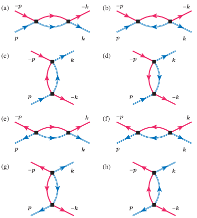
Figure 14: Equations for the dressed four-point vertices made out of $d$ and ${\bar{d}}$ bosons, at the second order in $J_{z}$. (a)–(d) Normal vertices $F^{(22)}$. (e)–(h) Anomalous vertices $F^{(04)}$.

We further compute irreducible interactions to second order in $J_{z}$. The corresponding contributions to $F^{(22)}({\bm{k}},{\bm{p}})$ and $F^{(04)}({\bm{k}},{\bm{p}})$ are shown in Fig. 14. We set external momenta at ${\bm{k}}={\bm{Q}},{\bm{p}}=\pm{\bm{Q}}$, but put no restriction on internal momenta. For practical purposes, we found it more convenient to evaluate directly the differences $\delta F^{(22)}=F^{(22)}({\bm{Q}},{\bm{Q}})-F^{(22)}({\bm{Q}},-{\bm{Q}})$ and $\delta F^{(04)}=F^{(04)}({\bm{Q}},{\bm{Q}})-F^{(04)}({\bm{Q}},-{\bm{Q}})$ rather than each term separately. In these notations, $A=\delta F^{(22)}-\delta F^{(04)}$.

The contributions to irreducible $\delta F^{(22)}$ at second order in $J_{z}$ come from three sets of processes: the one with two $2\to 2$ interactions, the one with $0\to 4$ and $4\to 0$ interactions, and the one with $1\to 3$ and $3\to 1$ interactions. Each of these interaction terms is obtained from the original interaction in terms of $a$ and $b$ bosons [Eq. (B)], by applying the transformation from $a,b$ to $d,{\bar{d}}$ bosons [Eq. (77)]. The $2\to 2$, $4\to 0$, and $0\to 4$ terms contain even numbers of $u$ and $v$ factors, $1\to 3$ and $3\to 1$ terms contain either three $u$ and one $v$ factor, or vice versa. As an example, we present the explicit expression for one of $3\to 1$ terms:

$$H_{3\to 1}=-\frac{J_{z}}{N}\sum_{1,2,3,4}d_{1}{\bar{d}}_{2}{\bar{d}}_{3}d_{4}K_{123,4}+....$$ (88)

where $1\equiv{\bm{k}}_{1}$, etc., momentum conservation is implied, and

$$K = \gamma_{1+3}\left[\left(u_{1}v_{3}-v_{1}u_{3}\right)\left(u_{2}u_{4}-v_{2}v_{4}\right)\right]$$ (89)

$$+\gamma_{1+2}\left[\left(u_{1}v_{2}-v_{1}u_{2}\right)\left(u_{3}u_{4}-v_{3}v_{4}\right)\right].$$

The ellipsis in (88) stands for other terms with $3\to 1$ structure.

Evaluating irreducible $\delta F^{(22)}$ and $\delta F^{(04)}$ from each of these processes and collecting combinatoric factors, we obtain

$$\delta F^{(22)}=-\frac{1}{4}J^{2}_{z}{\cal S},~{}~{}\delta F^{(04)}=\frac{1}{4}J^{2}_{z}{\cal S},$$ (90)

where

$${\cal S} =\frac{1}{N}\sum_{\bm{k}}\Bigg{[}\frac{\omega_{\bm{k}}}{2}\left(\gamma_{{\bm{Q}}+{\bm{k}}}-\gamma_{{\bm{Q}}-{\bm{k}}}\right)^{2}-\omega_{\bm{k}}~{}\gamma_{{\bm{Q}}+{\bm{k}}}\gamma_{{\bm{Q}}-{\bm{k}}}$$

$$\quad\qquad\quad+\frac{2\omega_{{\bm{Q}}+{\bm{k}}}\omega_{{\bm{Q}}-{\bm{k}}}}{\omega_{{\bm{Q}}+{\bm{k}}}+\omega_{{\bm{Q}}-{\bm{k}}}}\gamma^{2}_{\bm{k}}\Bigg{]}.$$ (91)

Numerical evaluation yields ${\cal S}=12.92J$, which is consistent with Eqs. (43) and (44) in the main text: $2{\cal S}=\sum_{i}\beta_{i}=\sum_{i}{\bar{\beta}}_{i}$. Using (85) and (90), we obtain $A=-6.46J^{2}_{z}J$. Substituting this $A$ into Eq. (84) we obtain

$$\frac{1}{3.23\zeta^{2}J^{3}}=\frac{1}{N}\sum_{\bm{p}}\frac{1}{\omega^{3}_{\bm{p}}}.$$ (92)

This is exactly the same equation as Eq. (47) in the main text, the only difference is that in the current approach $s^{2}=1$. [In Eq. (47), the numerical factor in the left-hand side is $\alpha=2.49=3.23s^{2}$.]

Using the fact that $(1/N)\sum_{\bm{p}}1/\omega^{3}_{\bm{p}}\sim(1/J^{3})(D/D_{c}-1)^{-1/2}$, the condition for the instability towards the CL state ($D=D^{b}_{c}$) takes the form

$$\frac{D^{b}_{c}}{D_{c}}-1\propto\left(\frac{J_{z}}{J}\right)^{4}=\zeta^{4}.$$ (93)

Because $D^{b}_{c}>D_{c}$, the instability towards the CL state pre-empts the one towards the magnetically ordered XY state. This again agrees with the finding in the main text. The difference in scaling of $D_{c}^{b}-D_{c}$ with Ising anisotropy $\zeta$ in (48) and (93), $\zeta^{2}$ vs $\zeta^{4}$, is due to different scaling forms of the minimal magnon energy, $\omega_{\bm{Q}}$, in the Schwinger boson approximation (main text) and the hard-core boson approximation (this appendix).

References

- Andreev and Grishchuk (1984) A. F. Andreev and I. A. Grishchuk, Zh. Eksp. Teor. Fiz. 87, 467 (1984), [JETP 60, 267 (1984)].
- Chubukov (1990a) A. V. Chubukov, Journal of Physics: Condensed Matter 2, 1593 (1990a).
- Penc and Läuchli (2011) K. Penc and A. M. Läuchli, “Spin nematic phases in quantum spin systems,” in Introduction to Frustrated Magnetism: Materials, Experiments, Theory, edited by C. Lacroix, P. Mendels, and F. Mila (Springer Berlin Heidelberg, Berlin, Heidelberg, 2011) pp. 331–362.
- Chandra et al. (1990a) P. Chandra, P. Coleman, and A. I. Larkin, Journal of Physics: Condensed Matter 2, 7933 (1990a).
- Chandra et al. (1990b) P. Chandra, P. Coleman, and A. I. Larkin, Phys. Rev. Lett. 64, 88 (1990b).
- Capriotti and Sachdev (2004) L. Capriotti and S. Sachdev, Phys. Rev. Lett. 93, 257206 (2004).
- Villain (1977) J. Villain, Journal de Physique 38, 385 (1977).
- Villain (1978) J. Villain, Annals of the Israel Physical Society 2, 565 (1978).
- Fradkin et al. (2010) E. Fradkin, S. A. Kivelson, M. J. Lawler, J. P. Eisenstein, and A. P. Mackenzie, Annual Review of Condensed Matter Physics 1, 153 (2010).
- Fernandes et al. (2012) R. M. Fernandes, A. V. Chubukov, J. Knolle, I. Eremin, and J. Schmalian, Phys. Rev. B 85, 024534 (2012).
- Kawamura (1998) H. Kawamura, Journal of Physics: Condensed Matter 10, 4707 (1998).
- Hasenbusch et al. (2005) M. Hasenbusch, A. Pelissetto, and E. Vicari, Journal of Statistical Mechanics: Theory and Experiment 2005, P12002 (2005).
- Korshunov (2006) S. E. Korshunov, Physics-Uspekhi 49, 225 (2006).
- Sorokin and Syromyatnikov (2012) A. O. Sorokin and A. V. Syromyatnikov, Phys. Rev. B 85, 174404 (2012).
- Schenck et al. (2014) H. Schenck, V. L. Pokrovsky, and T. Nattermann, Phys. Rev. Lett. 112, 157201 (2014).
- Sachdev (2001) S. Sachdev, Quantum Phase Transitions (Cambridge University Press, 2001).
- Kamiya et al. (2011) Y. Kamiya, N. Kawashima, and C. D. Batista, Phys. Rev. B 84, 214429 (2011).
- Parker and Balents (2017) E. Parker and L. Balents, Phys. Rev. B 95, 104411 (2017).
- Weber et al. (2003) C. Weber, L. Capriotti, G. Misguich, F. Becca, M. Elhajal, and F. Mila, Phys. Rev. Lett. 91, 177202 (2003).
- Nersesyan et al. (1998) A. A. Nersesyan, A. O. Gogolin, and F. H. L. Eßler, Phys. Rev. Lett. 81, 910 (1998).
- Kolezhuk and Vekua (2005) A. Kolezhuk and T. Vekua, Phys. Rev. B 72, 094424 (2005).
- Chubukov (1991) A. V. Chubukov, Phys. Rev. B 44, 4693 (1991).
- Hikihara et al. (2008) T. Hikihara, L. Kecke, T. Momoi, and A. Furusaki, Phys. Rev. B 78, 144404 (2008).
- Dhar et al. (2013) A. Dhar, T. Mishra, M. Maji, R. V. Pai, S. Mukerjee, and A. Paramekanti, Phys. Rev. B 87, 174501 (2013).
- Nersesyan (1991) A. A. Nersesyan, Physics Letters A 153, 49 (1991).
- Fjærestad and Marston (2002) J. O. Fjærestad and J. B. Marston, Phys. Rev. B 65, 125106 (2002).
- Hikihara et al. (2001) T. Hikihara, M. Kaburagi, and H. Kawamura, Phys. Rev. B 63, 174430 (2001).
- Greschner et al. (2013) S. Greschner, L. Santos, and T. Vekua, Phys. Rev. A 87, 033609 (2013).
- Momoi et al. (1997) T. Momoi, K. Kubo, and K. Niki, Phys. Rev. Lett. 79, 2081 (1997).
- Chubukov and Starykh (2013) A. V. Chubukov and O. A. Starykh, Phys. Rev. Lett. 110, 217210 (2013).
- Domenge et al. (2005) J.-C. Domenge, P. Sindzingre, C. Lhuillier, and L. Pierre, Phys. Rev. B 72, 024433 (2005).
- Wen et al. (1989) X. G. Wen, F. Wilczek, and A. Zee, Phys. Rev. B 39, 11413 (1989).
- Kalmeyer and Laughlin (1987) V. Kalmeyer and R. B. Laughlin, Phys. Rev. Lett. 59, 2095 (1987).
- Kalmeyer and Laughlin (1989) V. Kalmeyer and R. B. Laughlin, Phys. Rev. B 39, 11879 (1989).
- Schroeter et al. (2007) D. F. Schroeter, E. Kapit, R. Thomale, and M. Greiter, Phys. Rev. Lett. 99, 097202 (2007).
- Yao and Kivelson (2007) H. Yao and S. A. Kivelson, Phys. Rev. Lett. 99, 247203 (2007).
- Thomale et al. (2009) R. Thomale, E. Kapit, D. F. Schroeter, and M. Greiter, Phys. Rev. B 80, 104406 (2009).
- Gong et al. (2014) S.-S. Gong, W. Zhu, and D. N. Sheng, Scientific Reports 4, 6317 (2014).
- Zhu et al. (2014) W. Zhu, S. S. Gong, and D. N. Sheng, Journal of Statistical Mechanics: Theory and Experiment 2014, P08012 (2014).
- He et al. (2014) Y.-C. He, D. N. Sheng, and Y. Chen, Phys. Rev. Lett. 112, 137202 (2014).
- He and Chen (2015) Y.-C. He and Y. Chen, Phys. Rev. Lett. 114, 037201 (2015).
- Zhu et al. (2015) W. Zhu, S. S. Gong, and D. N. Sheng, Phys. Rev. B 92, 014424 (2015).
- Tewari et al. (2006) S. Tewari, D. Belitz, and T. R. Kirkpatrick, Phys. Rev. Lett. 96, 047207 (2006).
- Zapf et al. (2006) V. S. Zapf, D. Zocco, B. R. Hansen, M. Jaime, N. Harrison, C. D. Batista, M. Kenzelmann, C. Niedermayer, A. Lacerda, and A. Paduan-Filho, Phys. Rev. Lett. 96, 077204 (2006).
- Zapf et al. (2014) V. Zapf, M. Jaime, and C. D. Batista, Rev. Mod. Phys. 86, 563 (2014).
- Zaletel et al. (2014) M. P. Zaletel, S. A. Parameswaran, A. Rüegg, and E. Altman, Phys. Rev. B 89, 155142 (2014).
- Auerbach (1994) A. Auerbach, Interacting Electrons and Quantum Magnetism (Springer-Verlag, 1994).
- Muniz et al. (2014) R. A. Muniz, Y. Kato, and C. D. Batista, Prog. Theor. Exp. Phys. 2014, 083I01 (2014).
- Zhang et al. (2013) Z. Zhang, K. Wierschem, I. Yap, Y. Kato, C. D. Batista, and P. Sengupta, Phys. Rev. B 87, 174405 (2013).
- Holstein and Primakoff (1940) T. Holstein and H. Primakoff, Phys. Rev. 58, 1098 (1940).
- Kohn and Luttinger (1965) W. Kohn and J. M. Luttinger, Phys. Rev. Lett. 15, 524 (1965).
- Nakanishi (1969) N. Nakanishi, Prog. Theor. Phys. Suppl. 43, 1 (1969).
- Ueda and Momoi (2013) H. T. Ueda and T. Momoi, Phys. Rev. B 87, 144417 (2013).
- Katsura et al. (2005) H. Katsura, N. Nagaosa, and A. V. Balatsky, Phys. Rev. Lett. 95, 057205 (2005).
- Sergienko and Dagotto (2006) I. A. Sergienko and E. Dagotto, Phys. Rev. B 73, 094434 (2006).
- Mostovoy (2006) M. Mostovoy, Phys. Rev. Lett. 96, 067601 (2006).
- Janzen et al. (2016) P. Janzen, W.-M. Huang, and L. Mathey, Phys. Rev. A 94, 063614 (2016).
- Zhu et al. (2016) W. Zhu, S. S. Gong, and D. N. Sheng, Phys. Rev. B 94, 035129 (2016).
- Simon and Varma (2002) M. E. Simon and C. M. Varma, Phys. Rev. Lett. 89, 247003 (2002).
- Wang and Chubukov (2014) Y. Wang and A. Chubukov, Phys. Rev. B 90, 035149 (2014).
- Agterberg et al. (2015) D. F. Agterberg, D. S. Melchert, and M. K. Kashyap, Phys. Rev. B 91, 054502 (2015).
- Kleinert (1989) H. Kleinert, Gauge fields in condensed matter (World Scientific, Singapore, 1989).
- Blume (1966) M. Blume, Phys. Rev. 141, 517 (1966).
- Capel (1966) H. Capel, Physica 32, 966 (1966).
- Blume et al. (1971) M. Blume, V. J. Emery, and R. B. Griffiths, Phys. Rev. A 4, 1071 (1971).
- Mahan and Girvin (1978) G. D. Mahan and S. M. Girvin, Phys. Rev. B 17, 4411 (1978).
- Collins et al. (1988) J. B. Collins, P. A. Rikvold, and E. T. Gawlinski, Phys. Rev. B 38, 6741 (1988).
- Penrose and Onsager (1956) O. Penrose and L. Onsager, Phys. Rev. 104, 576 (1956).
- Ng and Lee (2006) K.-K. Ng and T. K. Lee, Phys. Rev. Lett. 97, 127204 (2006).
- Laflorencie and Mila (2007) N. Laflorencie and F. Mila, Phys. Rev. Lett. 99, 027202 (2007).
- Sengupta and Batista (2007a) P. Sengupta and C. D. Batista, Phys. Rev. Lett. 98, 227201 (2007a).
- Sengupta and Batista (2007b) P. Sengupta and C. D. Batista, Phys. Rev. Lett. 99, 217205 (2007b).
- Picon et al. (2008) J.-D. Picon, A. F. Albuquerque, K. P. Schmidt, N. Laflorencie, M. Troyer, and F. Mila, Phys. Rev. B 78, 184418 (2008).
- Peters et al. (2009) D. Peters, I. P. McCulloch, and W. Selke, Phys. Rev. B 79, 132406 (2009).
- Papanicolaou (1988) N. Papanicolaou, Nucl. Phys. B 305, 367 (1988).
- Chubukov (1989) A. V. Chubukov, Pis’ma Zh. Eksp. Teor. Fiz. 49, 108 (1989), [JETP Lett. 49, 129 (1989)].
- Chubukov (1990b) A. V. Chubukov, Journal of Physics: Condensed Matter 2, 4455 (1990b).
- Chubukov et al. (1991) A. V. Chubukov, K. I. Ivanova, P. C. Ivanov, and E. R. Korutcheva, Journal of Physics: Condensed Matter 3, 2665 (1991).
- Chubukov and Morr (1995) A. V. Chubukov and D. K. Morr, Phys. Rev. B 52, 3521 (1995).