3D Quantum Anomalous Hall Effect in Hyperhoneycomb Lattices

Abstract

We address the role of short range interactions for spinless fermions in the hyperhoneycomb lattice, a three dimensional (3D) structure where all sites have a planar trigonal connectivity. For weak interactions, the system is a line-node semimetal. In the presence of strong interactions, we show that the system can be unstable to a 3D quantum anomalous Hall phase with loop currents that break time reversal symmetry, as in the Haldane model. We find that the low energy excitations of this state are Weyl fermions connected by surface Fermi arcs. We show that the 3D anomalous Hall conductivity is $e^{2}/(\sqrt{3}ah)$, with $a$ the lattice constant.

Introduction. $-$ The quantum Hall conductivity describes dissipationless transport of electrons in a system that breaks time reversal symmetry (TRS) due to an external applied magnetic field. In two dimensions (2D), the current is carried through the edges Thouless1982 , and the Hall conductivity $\sigma_{xy}$ is quantized in units of $e^{2}/h$. In three dimensions (3D), the Hall conductivity is not universal and has an extra unit of inverse length. As shown by Halperin Halperin1987 , the 3D conductivity tensor on a lattice has the form $\sigma_{ij}=e^{2}/(2\pi h)\epsilon_{ijk}G_{k}$, where $G$ is a reciprocal lattice vector (it could be zero). The realization of the 3D quantum Hall effect has been proposed in systems with very anisotropic Fermi surfaces Balicas ; McKerman ; Bernevig , or else in line-node semimetals Guinea ; Mullen2015 ; Moessner ; Kim , where the Fermi surface has the form of a line of Dirac nodes Burkov ; Lu ; Yang ; Rappe ; Weng ; Yu ; Heykikila ; Chen ; Ezawa ; Wang ; Bian ; Bian2 ; Chan ; Xie ; Li .

Equally interesting would be to realize the 3D quantum anomalous Hall (QAH) effect Xu ; Xu2 , where the anomalous Hall conductivity emerges from the topology of the 3D band structure in the absence of Landau levels. The first proposal for a Chern insulator system was the Haldane model Haldane1988 on the honeycomb lattice, where loop currents break TRS and can produce a non-zero Chern number in the bulk states. Hyperhoneycomb lattices have the same planar trigonal connectivity of the honeycomb lattice (see Fig. 1a), and hence could provide a natural system for the emergence of a 3D QAH conductivity. This lattice has been experimentally realized in honeycomb iridates Modic as a candidate for the Kitaev model Kitaev and awaits to be realized as a line-node semimetal.

In this Letter, we describe the 3D QAH state that emerges from interactions in a hyperhoneycomb lattice with spinless fermions. This state competes with a CDW state, and produces a very anisotropic gap around a line of Dirac nodes in the semimetallic state. Due to a broken inversion symmetry, the QAH gap changes sign along the nodal line, forming Weyl points connected by Fermi arcs Wan ; Armitage . We show that the QAH conductivity of the surface states is $e^{2}/(\sqrt{3}ah)$, with $a$ the lattice constant.

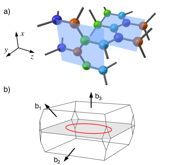
Figure 1: (color online) a) Hyperhoneycomb lattice with four sublattices, indicated by the different color sites. All sites are trigonally connected with planar links spaced by $120^{\circ}$. The two planes are rotated by $\pi/2$ along the $z$ direction, which has a screw symmetry. b) 3D Brillouin zone of the crystal. In the semi-metallic state, a closed zero energy line of Dirac nodes (Dirac loop) is shown in the red curve on the $k_{z}=0$ plane (gray area). The black arrows indicate the reciprocal lattice vectors.

Lattice model.$-$ We start from the tight binding model of the hyperhoneycomb lattice, which has four atoms per unit cell and planar links spaced by $120^{\circ}$, as shown in Fig. 1a. The lattice has three vector generators $\mathbf{a}_{1}=(\sqrt{3},0,0)$, $\mathbf{a}_{2}=(0,\sqrt{3},0)$ and $\mathbf{a}_{3}=(-\sqrt{3}/2,\sqrt{3}/2,3)$, and the corresponding reciprocal lattice vectors $\mathbf{b}_{1}=(2\pi/\sqrt{3},0,-\pi/3)$, $\mathbf{b}_{2}=(0,-2\pi/\sqrt{3},\pi/3)$ and $\mathbf{b}_{3}=(0,0,2\pi/3)$. For a model of spinless fermions, which could physically result from a strong Rashba spin orbit coupling, the kinetic energy is $\mathcal{H}_{0}=-t\sum_{\left\langle i,j\right\rangle}(a_{i}^{\dagger}a_{j}+h.c.)$, where $a_{i}$ destroys an electron on site $i$, $t$ is the hopping energy and $\langle ij\rangle$ denotes nearest neighbor (NN) sites. In the four-sublattice basis, the Hamiltonian is a 4$\times$4 matrix Mullen2015

$$\mathcal{H}_{0}=-t\left(\begin{array}[]{cccc}0&\Theta_{x}&0&\text{e}^{ik_{z}}\\ \Theta_{x}^{*}&0&\text{e}^{-ik_{z}}&0\\ 0&\text{e}^{ik_{z}}&0&\Theta_{y}\\ \text{e}^{-ik_{z}}&0&\Theta_{y}^{*}&0\end{array}\right),$$ (1)

where $\Theta_{\gamma}\equiv 2\text{e}^{ik_{z}/2}\cos(\sqrt{3}k_{\gamma}/2)$, with $\gamma=x,\,y$, and $\mathbf{k}$ is the momentum away from the center of the Brillouin zone (BZ). The electronic structure has a doubly degenerate zero energy line of nodes in the form of a Dirac loop at the $k_{z}=0$ plane, $\mathbf{k}_{0}(s)\equiv(k_{x}(s),k_{y}(s),0)$ in some parametrization that satisfies the equation $4\cos(\sqrt{3}k_{x}(s)/2)\cos(\sqrt{3}k_{y}(s)/2)=1$, as schematically depicted in Fig. 1b. The projected low energy Hamiltonian has the form

$$\mathcal{H}_{0,p}(\mathbf{q})=\left[v_{x}(s)q_{x}+v_{y}(s)q_{y}\right]\sigma_{x}+v_{z}(s)q_{z}\sigma_{y},$$ (2)

where $\mathbf{q}\equiv\mathbf{k}-\mathbf{k}_{0}(s)$ is the momentum away from the nodal line, $\sigma_{x},\,\sigma_{y}$ are Pauli matrices, with $v_{x}(s)=\frac{\sqrt{3}}{2}t\sin(\sqrt{3}k_{x}(s)/2)/(1+\alpha^{2})$, $v_{y}(s)=\frac{\sqrt{3}}{2}\alpha^{2}t\sin(\sqrt{3}k_{y}(s)/2)/(1+\alpha^{2})$ and $v_{z}=-3t\alpha/(1+\alpha^{2})$ the quasiparticle velocities, and $\alpha(s)=2\cos(\sqrt{3}k_{x}(s)/2)$. Hamiltonian (2) corresponds to the low energy spectrum

$$\epsilon_{0}(\mathbf{q})=\sqrt{(v_{x}q_{x}+v_{y}q_{y})^{2}+v_{z}^{2}q_{z}^{2}},$$ (3)

that is gapless along the nodal line.

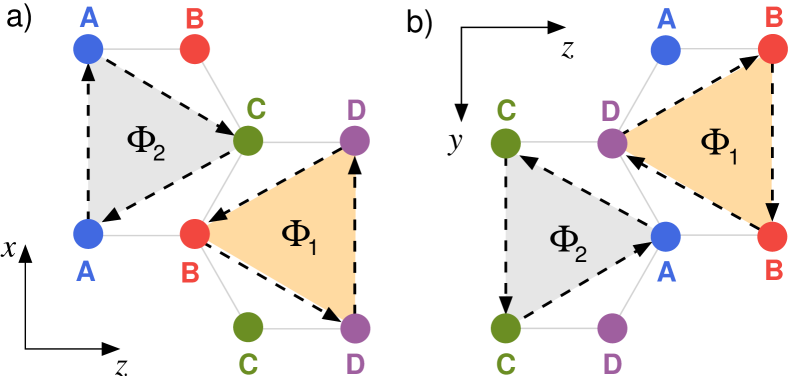
Figure 2: (color online) $xz$ (a) and $yz$ (b) planes of the hyperhoneycomb lattice, with sublattices $A,\,B\,,C$ and $D$. Complex NNN hopping terms $\chi_{ij}$ give rise to current loops with flux $\Phi$. The lowest energy state has $\Phi_{1}=-\Phi_{2}$, which corresponds to a zero total flux in the unit cell, with purely imaginary $\chi_{ij}$.

The total Hamiltonian is $\mathcal{H}=\mathcal{H}_{0}+\mathcal{H}_{I}$, where

$$\mathcal{H}_{I}=V_{1}\!\sum_{\left\langle i,j\right\rangle}(\hat{n}_{i}-1)(\hat{n}_{j}-1)+V_{2}\negthickspace\!\sum_{\left\langle\left\langle i,j\right\rangle\right\rangle}(\hat{n}_{i}-1)(\hat{n}_{j}-1),$$ (4)

is the interaction term, with $\hat{n}_{i}=a_{i}^{\dagger}a_{i}$ the density operator on site $i$, and $V_{1}$ and $V_{2}$ are the repulsion between NN and next-nearest neighbors (NNN) sites, respectively. For spinless fermions, one possible instability is a charge density wave (CDW) state that corresponds to a charge imbalance among the different sublattices. The CDW state is defined by the four component order parameter $\rho_{\alpha}=\langle a_{i}^{\dagger}a_{i}\rangle-\rho_{0}$ with $i\in\alpha$ belonging to sublattice $\alpha=A\,,B,\,C,\,D$, as shown in Fig 2, and $\rho_{0}$ a uniform density. At the neutrality point, the local densities at the four sites of the unit cell add up to zero, $\sum_{\alpha}\rho_{\alpha}=0$. The nodal line is protected by a combination of TRS and mirror symmetry along the $z$ axis. The state where $\rho_{A}=-\rho_{B}=\rho_{C}=-\rho_{D}$, namely $(\rho,-\rho,\rho,-\rho)$, breaks the mirror symmetry and opens the largest gap among all possible charge neutral configurations of $\rho_{\alpha}$. The more symmetric state $(\rho,\rho,-\rho,-\rho)$ does not open a gap. Hence, the former state is the dominant CDW instability. We will not consider other possible states that enlarge the size of the unit cell Grushin , such as an $n$-site CDW state, with $n>4$.

The other dominant instability is the QAH state, where complex hopping terms between NNN sites lead to loop currents in the $xz$ and $yz$ planes, as shown in Fig. 2. Each plane can have loop currents with opposite flux ($\Phi$), producing zero magnetic flux in the unit cell, in analogy with the 2D case in the honeycomb lattice Haldane1988 . The QAH order parameter is defined as $\chi_{ij}=\langle a_{i}^{\dagger}a_{j}\rangle$, where $i$ and $j$ sites are connected by NNN vectors Raghu2008 . We define the Ansatz $\chi_{ij}=\chi\text{e}^{i\phi_{ij}}$ for $i,\,j\in\{A,\,C\}$ sublattices and $\chi_{ij}=\chi\text{e}^{i\bar{\phi}_{ij}}$ for $i,\,j\in\{B,D\}$, where $\chi$ is real. Due to particle-hole symmetry, $\chi_{ij}$ is purely imaginary and hence $\phi,\bar{\phi}=\pm\frac{\pi}{2}$. The state that minimizes the free energy of the system has total zero flux in the unit cell, $\Phi_{1}=-\Phi_{2}$ (see Fig. 2), when the magnetic flux lines can more easily close. The QAH order parameter is $\chi_{ij}=\pm i\chi$ for NNN sites and zero otherwise, with the $+$ sign following the convention of the arrows in Fig. 2.

We perform a mean-field decomposition of the NN interaction in the CDW state ($\rho$) and of the NNN repulsion in the QAH order parameter $\chi_{ij}$. For simplicity, we absorb the couplings $V_{1}$ and $V_{2}$ in the definition of the order parameters, $\rho V_{1}\to\rho$ and $\chi V_{2}\to\chi$, which have units of energy from now on. The effective interaction in the four-sublattice basis is

$$\mathcal{H}_{I}^{{\rm MF}}=\left(\begin{array}[]{cccc}\chi g-3\rho&0&-\chi f&0\\ 0&-\chi g+3\rho&0&\chi f^{*}\\ -\chi f^{*}&0&\chi g-3\rho&0\\ 0&\chi f&0&-g\chi+3\rho\end{array}\right)\!,$$ (5)

where

$$g(\mathbf{k})=2\left[\sin\left(\sqrt{3}k_{x}\right)+\sin\left(\sqrt{3}k_{y}\right)\right],$$ (6)

and

$$f(\mathbf{k})=2\left[\text{e}^{i3k_{z}/2}\sin\left(\sqrt{3}k_{x}/2\right)+\text{e}^{-i3k_{z}/2}\sin\left(\sqrt{3}k_{y}/2\right)\right].$$ (7)

The mean-field Hamiltonian $\mathcal{H}^{\text{MF}}=\mathcal{H}_{0}+\mathcal{H}_{I}^{\text{MF}}$ has an additional constant energy term $E_{0}=6\rho^{2}/V_{1}+16\chi^{2}/V_{2}$ that is reminiscent of the decomposition of the interactions to quadratic form.

The phase diagram follows from the numerical minimization of the free energy $F$ with respect to $\rho$ and $\chi$ at zero temperature, $\partial F/\partial\chi=\partial F/\rho=0$. The semimetal state is unstable to a CDW order at the critical coupling $V_{1,c}=0.41t$, and to a QAH phase at $V_{2,c}=1.51t$. The CDW and QAH states compete with each other, as shown in Fig. 3. Fluctuation effects are expected to be less dramatic in 3D compared to the more conventional 2D case Raghu2008 ; Motruck ; Scherer . Hence, the mean-field phase diagram is likely a reliable indication of the true instabilities of the fermionic lattice for the spinless case.

In real crystals, screening and elastic effects lead to a distortion of the lattice in the CDW state, in order to minimize the Coulomb energy due to electron-ion coupling, which can be high Cowley . While the CDW appears to be the leading instability over the QAH state, the elastic energy cost to displace the ions and equilibrate the charge in the electron-ion system may hinder the CDW order and favor the QAH phase when $V_{2}>V_{2,c}$.

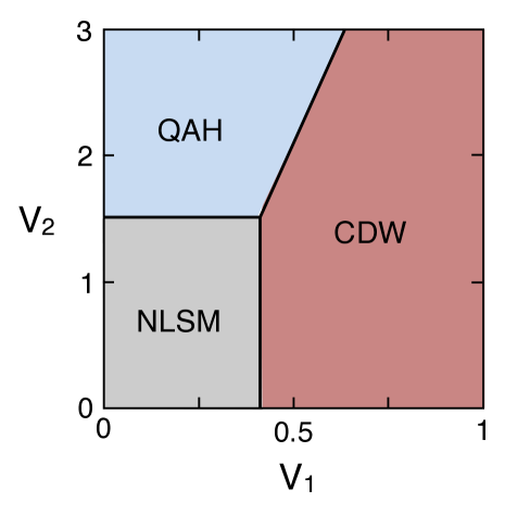
Figure 3: (color online) a) Mean field phase diagram for spinless fermions. The node-line semimetal phase (NLSM) turns into the CDW state at the critical value $V_{1}=0.41t$ and into the QAH phase in 3D at $V_{2}=1.51t$. The CDW is fully gapped, while the QAH phase has nodes around the Dirac loop.

Low energy Hamiltonian$.-$Integrating out the two high energy bands using perturbation theory, the effective low energy Hamiltonian (2) of the nodal line becomes massive, as expected. The leading correction to Hamiltonian (2) around the nodal line to lowest order in $\rho$ and $\chi$ has the form of a mass term

$$\mathcal{H}_{I,p}\left(\mathbf{q}\right)=-\left[3\rho+m(\mathbf{k}_{0})+v_{x}^{\prime}q_{x}+v_{y}^{\prime}q_{y}\right]\sigma_{3},$$ (8)

where

$$m(\mathbf{k}_{0})=\chi\left(g(\mathbf{k}_{0})+\frac{2}{\alpha+\frac{1}{\alpha}}f(\mathbf{k}_{0})\right)$$ (9)

gives the QAH mass at the nodal line, with $v_{\gamma}^{\prime}(s)=2\chi\{\cos(\sqrt{3}k_{\gamma}(s))+\frac{1}{\alpha+1/\alpha}\cos(\sqrt{3}k_{\gamma}(s)/2)\}$ and $\alpha(s)$ defined below Eq. (2). The low energy spectrum is

$$\epsilon(\mathbf{q})=\pm\sqrt{\epsilon_{0}^{2}(\mathbf{q})+\left[3\rho+m(\mathbf{k}_{0})+v_{x}^{\prime}q_{x}+v_{y}^{\prime}q_{y}\right]^{2}},$$ (10)

which describes either a uniformly gapped state in the CDW phase ($\rho\neq 0$, $\chi=0$) or a non-uniform QAH gap $(\rho=0,\chi\neq 0)$ with six nodes at the zeros of $m(\mathbf{k}_{0})$, as indicated in Fig. 4.

The CDW state breaks mirror symmetry along the $z$ axis, but preserves the screw axis symmetry and hence creates a fully gapped state that is rotationally symmetric along the nodal line. The QAH state on the order hand breaks inversion symmetry. The mass term (9) changes sign at six zeros along the nodal line, as shown in Fig. 4b. Two zeros are located along the diagonal direction of the nodal line, at the points $\pm\mathbf{Q}_{1}=\pm\left(-\frac{2\pi}{3\sqrt{3}},\frac{2\pi}{3\sqrt{3}},0\right)$. The other four zeros of $m(\mathbf{k}_{0})$ are symmetrically located around that direction, at $\pm\mathbf{Q}_{2}=\pm(Q_{+},Q_{-},0)$ and $\pm\mathbf{Q}_{3}=\mp(Q_{-},Q_{+},0)$, as shown in Fig. 4, with $Q_{\pm}=\frac{1}{\sqrt{3}}\text{arccos}(\frac{\sqrt{17}-1}{4})\pm\frac{1}{\sqrt{3}}\arccos(\frac{3-\sqrt{17}}{4})$. The position of the nodal points extracted from the low energy Hamiltonian (8) is in agreement with the values calculated numerically from Hamiltonians (1) and (5) in the regime where $\chi\ll t$. For larger values of $\chi$, the nodal points $\pm\mathbf{Q}_{2}$ and $\pm\mathbf{Q}_{3}$ can move in the $k_{z}=0$ plane, as the position of the nodal line is renormalized by the interactions. The two nodal points in the diagonal $\pm\mathbf{Q}_{1}$ remain fixed.

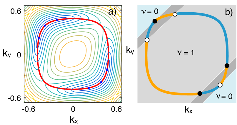
Figure 4: (color online) a) Contour plot of the mass gap of the QAH state (9) around the Dirac loop (red line). Momenta are in units of $\pi$. The gap vanishes at six points along the nodal line indicated by the blue dots, where the contours collapse. b) Schematic picture of the sign of the QAH gap around the nodal line: blue line ($m>0$); orange line ($m<0$). At the nodes, the low energy excitations are Weyl fermions, with helicities $\gamma=+1$ (black dots) and $\gamma=-1$ (white). The Weyl points are intercepted by four planes oriented in the $(1\bar{1}0)$ direction (diagonal lines). Those planes form domain walls separating slices of the BZ with distinct Chern numbers. Gray area: $\nu=1$. Dark gray: $\nu=-1$. Light blue: $\nu=0$.

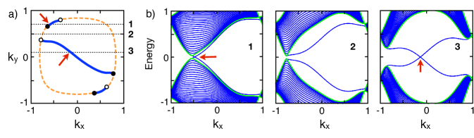
Figure 5: (color online) a) Fermi arcs on the (001) surface BZ indicated by the blue solid lines. The brown dashed represents the nodal ring in the bulk in the absence of interactions. The black and white circles are the Weyl nodes in the bulk with positive and negative helicities. b) Panels showing the energy dispersions $E(k_{x},k_{y})$ along the three momentum space cuts labeled $1,\,2,\,3$, indicated in panel a. All momenta are in units of $\pi/\sqrt{3}$ and energy has units of the hopping energy $t$. (left) cut 1, with $k_{y}=3\pi/(4\sqrt{3})$; (center) cut $2$, with $k_{y}=\pi/(2\sqrt{3})$, where there is no Fermi arc; (right) cut $3$, with $k_{y}=\pi/(10\sqrt{3})$. Red arrows indicate the zero energy modes on the surface BZ.

Expanding the the mass term around the zeros of $m(\mathbf{k}_{0})$, the low energy quasiparticles around the nodes are Weyl fermions. Performing a rotation of the quasiparticle momenta into a new basis $p_{x}=(q_{x}-q_{y})/\sqrt{2},$ $p_{y}=-q_{z}$ and $p_{z}=(q_{x}+q_{y})/\sqrt{2}$, the expansion around the the nodes at $\pm\mathbf{Q}_{1}$ gives the low energy Hamiltonian

$$\mathcal{H}_{\pm Q_{1}}(\mathbf{p})=\mathbf{h}_{\pm Q_{1}}(\mathbf{p})\cdot\vec{\sigma}=\sum_{i=x,y,z}v_{0,i}^{(\pm)}p_{i}\sigma_{i},$$ (11)

with $\mathbf{p}$ the momentum away from the nodes and $v_{0,x}^{(\pm)}=\pm 3\sqrt{2}t/4,\>v_{0,y}=3t/2$ and $v_{0,z}=\sqrt{3/2}\chi$ the corresponding velocities in the rotated basis. The equation above describes two Weyl points with opposite helicities $\gamma=(2\pi)^{-2}\int_{\Omega}\text{d}^{2}p\,\hat{h}\cdot(\partial_{p_{x}}\hat{h}\times\partial_{p_{y}}\hat{h})=\pm 1$, and hence broken TRS, with $\hat{h}=\mathbf{h}/|\mathbf{h}|$ a unitary vector and $\Omega$ the surface of a small sphere enclosing each node. Similarly, the expansion around the nodes $\pm\mathbf{Q}_{2}$ and $\pm\mathbf{Q}_{3}$ give Hamiltonians of Weyl fermions with helicities $\pm 1$, as indicated in Fig. 4b.

Anomalous Hall conductivity$.-$ The Weyl points delimit a topological domain wall between slices of the BZ parallel to the $(1\bar{1}0)$ plane. Each slice in the light gray region in Fig. 4b crosses the nodal line twice and has a well defined Chern number $\nu=+1$. The slices in the dark gray regions across the domain walls have opposite Chern number $\nu=-1$, as the QAH mass changes sign simultaneously at the two Weyl points (with the same helicity) where each domain wall intersects the nodal line. The BZ slices in the light blue region do not cross the nodal line and have zero Chern number.

The 3D QAH conductivity is defined as $\sigma_{ij}=(e^{2}/h)(2\pi)^{-3}\int_{BZ}\text{d}^{3}k\sum_{n\in\textrm{filled}}(\frac{\partial}{\partial k_{i}}A_{j}-\frac{\partial}{\partial k_{j}}A_{i})$, where $A_{j}=-i\left\langle\psi_{n}\right|\frac{\partial}{\partial k_{j}}\left|\psi_{n}\right\rangle$ is the Berry connection of the $n$-th occupied Block band integrated over the entire BZ Haldane2 . For the hyperhoneycomb lattice in the QAH state,

$$\sigma_{ij}=\frac{e^{2}}{2\pi h}\int_{C}\text{d}k_{k}\epsilon_{ijk}\nu_{(k)}(\mathbf{k}_{0})=\frac{e^{2}}{2\pi h}\epsilon_{ijk}(\mathbf{b}_{1}+\mathbf{b}_{2})_{k},$$ (12)

where $\mathbf{b}_{1}+\mathbf{b}_{2}=\left(2\pi/\sqrt{3},-2\pi/\sqrt{3},0\right)a^{-1}$ is a reciprocal lattice vector, restoring the lattice constant $a$. $\nu_{(j)}(\mathbf{k}_{0})=0,\,\pm 1$ is the Chern number of a slice of the BZ oriented in the $j=x,y,z$ direction, intersecting the nodal line $\mathbf{k}_{0}(s)$ at two points, and $C\in[k_{j,\text{min}}(s),k_{j,\text{max}}(s)]$. Therefore, we find that

$$\sigma_{yz}=\sigma_{xz}=e^{2}/(\sqrt{3}ha),$$ (13)

while $\sigma_{xy}=0$. In the 3D QAH phase, the bulk of the system is a semimetal with topologically protected Weyl quasiparticles Xu , while charge currents spontaneously emerge on the $[100]$ and $[010]$ surfaces of the crystal.

Surface states$.-$ The presence of Weyl points in the QAH state implies in the existence of Fermi arcs on the surfaces of the lattice, connecting nodes with opposite helicities. In Fig. 5a, we numerically calculate the Fermi arcs in the (001) surface Brillouin zone, as shown in the solid blue lines. The nodes at $\pm\mathbf{Q}_{2}$ are connected by a Fermi arc crossing the center of the BZ, while the pair of nodes at $\mathbf{Q}_{1}$, $-\mathbf{Q}_{3}$ and $-\mathbf{Q}_{1}$, $\mathbf{Q}_{3}$ are connected by short Fermi arcs directed along the nodal line.

In Fig. 5b, we scan the energy spectrum of the $k_{z}=0$ plane along the $k_{x}$ axis along three paths indicated by the dotted horizontal lines in panel 5a. Line 1 ($k_{y}=3\pi/(4\sqrt{3}$) intersects a Fermi arc close to the node at $\mathbf{Q}_{1}$, as indicated by the arrow in the left panel of Fig. 5b, which has a zero energy crossing in the vicinity of a node. The scan on line 2, at $k_{y}=\pi/(2\sqrt{3})$, does not intercept a Fermi arc, as shown in the center panel of Fig. 5b. The third path at $k_{y}=\pi/(10\sqrt{3})$ crosses the Fermi arc near the center of the zone, as indicated by the zero energy mode shown in the right panel of Fig. 5b.

Conclusions$.-$ We have shown that hyperhoneycomb lattices with spinless fermions may host a 3D QAH effect, which competes with a CDW state. The 3D anomalous Hall conductivity is $e^{2}/(\sqrt{3}ha)$. Due to the symmetry of the mass term, which spontaneously breaks inversion symmetry around the nodal line, the low energy excitations of the QAH state have a rich structure, with Weyl fermions in bulk and topologically protected surface states.

Acknowledgements.$-$ We acknowledge F. Assaad, S. Parameswaran and K. Mullen for helpful discussions. S. W. Kim and B.U. acknowledge NSF CAREER Grant No. DMR- 1352604 for support. K. S. acknowledges the University of Oklahoma for support.

Note.$-$ Recently, we became aware of a related work Murakami , which predicted the conditions for the emergence of Weyl points in nodal-line semimetals from symmetry arguments.

References

- (1) D. J. Thouless, M. Kohmoto, M. P. Nightingale, and M. Den Nijs, Phys. Rev. Lett. 49, 405 (1982).
- (2) B. I. Halperin, Jpn. J. Appl. Phys. 26 (1987).
- (3) L. Balicas, G. Kriza, and F. I. B. Williams, Phys. Rev. Lett. 75, 2000 (1995).
- (4) S. K. McKernan, S. T. Hannahs, U. M. Scheven, G. M. Danner, and P.M. Chaikin, Phys. Rev. Lett. 75, 1630 (1995).
- (5) B. A. Bernevig, T. L. Hughes, S. Raghu, and D. P. Arovas, Phys. Rev. Lett. 99, 146804 (2007).
- (6) F. Guinea and D. Arovas, Phys. Rev. B 78, 245416 (2008).
- (7) K. Mullen, B. Uchoa, and D. T. Glatzhofer, Phys. Rev. Lett. 115, 026403 (2015).
- (8) L.-K. Lim and R. Moessner, Phys. Rev. Lett. 118, 016401 (2017).
- (9) J.-W. Rhim and Y. B. Kim, Phys. Rev. B 92, 045126 (2015).
- (10) A. A. Burkov, M. D. Hook and L. Balents, Phys. Rev. B 84, 235126 (2011).
- (11) L. Lu, L. Fu, J. D. Joannopoulos and M. Soljačić, Nat. Photonics 7, 294 (2013).
- (12) S. A. Yang, H. Pan, and F. Zhang, Phys. Rev. Lett. 113, 046401 (2014).
- (13) Y. Kim, B. J. C. Wieder, C. L. Kane, and A. Rappe, Phys. Rev. Lett. 115, 036806 (2015).
- (14) H. Weng, Y. Liang, Q. Xu, Y. Rui, Z. Fang, X. Dai and Y. Kawa, Phys. Rev. B 92, 045108 (2015).
- (15) R. Yu, H. Weng, Z. Fang, X. Dai, and X. Hu, Phys. Rev. Lett. 115, 036807 (2015).
- (16) T. T. Heikkila and G. E. Volovik, JETP Lett. 93, 59 (2011).
- (17) Y. Chen, Y. Xie, S. A. Yang, H. Pan, F. Zhang, M. L. Cohen, and S. Zhang, Nano Letters 15, 6974 (2015).
- (18) L. S. Xie, L. M. Schoop, E. M. Seibel, Q. D. Gibson, W. Xie, and R. J. Cava, APL Mater. 3, 083602 (2015).
- (19) M. Ezawa, Phys. Rev. Lett. 116, 127202 (2016).
- (20) J.-T. Wang, H. Weng, S. Nie, Z. Fang, Y. Kawazoe, and C. Chen, Phys. Rev. Lett. 116, 195501 (2016).
- (21) G. Bian et.al., Nat. Commun. 7, 10556 (2016).
- (22) G. Bian et al., Phys. Rev. B 93, 121113(R) (2016).
- (23) Y.-H. Chan, C.-K. Chiu, M.Y. Chou, and A. P. Schnyder, Phys. Rev. B 93, 205132 (2016).
- (24) R. Li, H. Ma, X. Cheng, S. Wang, D. Li, Z. Zhang, Y. Li, and X.-Q. Chen, Phys. Rev. Lett. 117, 096401 (2016).
- (25) G. Xu, H. Weng, Z. Wang, X. Dai, and Z. Fang, Phys. Rev. Lett. 107, 186806 (2011).
- (26) G. Xu, J. Wang, C. Felser, X.-L. Q, and S.-C. Zhang, Nano Lett. 15, 2019 (2015).
- (27) F. D. M. Haldane, Phys. Rev. Lett. 61, 18 (1988).
- (28) K. A Modic et al., Nat. Commun. 5, 1 (2014).
- (29) A. Kitaev, Ann. Phys. (Amsterdam) 321, 2 (2006).
- (30) X. Wan, A. M. Turner, A. Vishwanath, and S. Y. Savrasov, Phys. Rev. B 83, 205101 (2011).
- (31) N. P. Armitage, E. J. Mele, Ashvin Vishwanath, arXiv:1705.01111 (2017).
- (32) A. G. Grushin, E. V. Castro, A. Cortijo, F. de Juan, M. A. H. Vozmediano, B. Valenzuela, Phys. Rev. B 87, 085136 (2013).
- (33) S. Raghu, X.-L. Qi, C. Honerkamp, and S.-C. Zhang, Phys. Rev. Lett. 100 156401 (2008).
- (34) J. Motruk, A.G. Grushin, F. de Juan, and F. Pollmann, Phys. Rev. B 92, 085147 (2015).
- (35) D.D. Scherer, M.M. Scherer, C. Honerkamp, Phys. Rev. B 92, 155137 (2015).
- (36) R. D. Cowley, Adv. Phys. 29, 1 (1980).
- (37) F. D. M. Haldane Phys. Rev. Lett. 93, 206602 (2004).
- (38) R. Okugawa and S. Murakami, arXiv:1706.08551 (2017).